STAR Collaboration

$\Delta\phi\Delta\eta$ Correlations in Central Au+Au Collisions at $\sqrt{s_{NN}}=$ 200 GeV

J. Adams University of Birmingham, Birmingham, United Kingdom M.M. Aggarwal Panjab University, Chandigarh 160014, India Z. Ahammed Variable Energy Cyclotron Centre, Kolkata 700064, India J. Amonett Kent State University, Kent, Ohio 44242 B.D. Anderson Kent State University, Kent, Ohio 44242 M. Anderson University of California, Davis, California 95616 D. Arkhipkin Particle Physics Laboratory (JINR), Dubna, Russia G.S. Averichev Laboratory for High Energy (JINR), Dubna, Russia Y. Bai NIKHEF and Utrecht University, Amsterdam, The Netherlands J. Balewski Indiana University, Bloomington, Indiana 47408 O. Barannikova Purdue University, West Lafayette, Indiana 47907 L.S. Barnby University of Birmingham, Birmingham, United Kingdom J. Baudot Institut de Recherches Subatomiques, Strasbourg, France S. Bekele Ohio State University, Columbus, Ohio 43210 V.V. Belaga Laboratory for High Energy (JINR), Dubna, Russia A. Bellingeri-Laurikainen SUBATECH, Nantes, France R. Bellwied Wayne State University, Detroit, Michigan 48201 B.I. Bezverkhny Yale University, New Haven, Connecticut 06520 S. Bhardwaj University of Rajasthan, Jaipur 302004, India A. Bhasin University of Jammu, Jammu 180001, India A.K. Bhati Panjab University, Chandigarh 160014, India H. Bichsel University of Washington, Seattle, Washington 98195 J. Bielcik Yale University, New Haven, Connecticut 06520 J. Bielcikova Yale University, New Haven, Connecticut 06520 L.C. Bland Brookhaven National Laboratory, Upton, New York 11973 C.O. Blyth University of Birmingham, Birmingham, United Kingdom S-L. Blyth Lawrence Berkeley National Laboratory, Berkeley, California 94720 B.E. Bonner Rice University, Houston, Texas 77251 M. Botje NIKHEF and Utrecht University, Amsterdam, The Netherlands J. Bouchet SUBATECH, Nantes, France A.V. Brandin Moscow Engineering Physics Institute, Moscow Russia A. Bravar Brookhaven National Laboratory, Upton, New York 11973 M. Bystersky Nuclear Physics Institute AS CR, 250 68 Řež/Prague, Czech Republic R.V. Cadman Argonne National Laboratory, Argonne, Illinois 60439 X.Z. Cai Shanghai Institute of Applied Physics, Shanghai 201800, China H. Caines Yale University, New Haven, Connecticut 06520 M. Calderón de la Barca Sánchez University of California, Davis, California 95616 J. Castillo NIKHEF and Utrecht University, Amsterdam, The Netherlands O. Catu Yale University, New Haven, Connecticut 06520 D. Cebra University of California, Davis, California 95616 Z. Chajecki Ohio State University, Columbus, Ohio 43210 P. Chaloupka Nuclear Physics Institute AS CR, 250 68 Řež/Prague, Czech Republic S. Chattopadhyay Variable Energy Cyclotron Centre, Kolkata 700064, India H.F. Chen University of Science & Technology of China, Hefei 230026, China J.H. Chen Shanghai Institute of Applied Physics, Shanghai 201800, China Y. Chen University of California, Los Angeles, California 90095 J. Cheng Tsinghua University, Beijing 100084, China M. Cherney Creighton University, Omaha, Nebraska 68178 A. Chikanian Yale University, New Haven, Connecticut 06520 H.A. Choi Pusan National University, Pusan, Republic of Korea W. Christie Brookhaven National Laboratory, Upton, New York 11973 J.P. Coffin Institut de Recherches Subatomiques, Strasbourg, France T.M. Cormier Wayne State University, Detroit, Michigan 48201 M.R. Cosentino Universidade de Sao Paulo, Sao Paulo, Brazil J.G. Cramer University of Washington, Seattle, Washington 98195 H.J. Crawford University of California, Berkeley, California 94720 D. Das Variable Energy Cyclotron Centre, Kolkata 700064, India S. Das Variable Energy Cyclotron Centre, Kolkata 700064, India M. Daugherity University of Texas, Austin, Texas 78712 M.M. de Moura Universidade de Sao Paulo, Sao Paulo, Brazil T.G. Dedovich Laboratory for High Energy (JINR), Dubna, Russia M. DePhillips Brookhaven National Laboratory, Upton, New York 11973 A.A. Derevschikov Institute of High Energy Physics, Protvino, Russia L. Didenko Brookhaven National Laboratory, Upton, New York 11973 T. Dietel University of Frankfurt, Frankfurt, Germany P. Djawotho Indiana University, Bloomington, Indiana 47408 S.M. Dogra University of Jammu, Jammu 180001, India W.J. Dong University of California, Los Angeles, California 90095 X. Dong University of Science & Technology of China, Hefei 230026, China J.E. Draper University of California, Davis, California 95616 F. Du Yale University, New Haven, Connecticut 06520 V.B. Dunin Laboratory for High Energy (JINR), Dubna, Russia J.C. Dunlop Brookhaven National Laboratory, Upton, New York 11973 M.R. Dutta Mazumdar Variable Energy Cyclotron Centre, Kolkata 700064, India V. Eckardt Max-Planck-Institut für Physik, Munich, Germany W.R. Edwards Lawrence Berkeley National Laboratory, Berkeley, California 94720 L.G. Efimov Laboratory for High Energy (JINR), Dubna, Russia V. Emelianov Moscow Engineering Physics Institute, Moscow Russia J. Engelage University of California, Berkeley, California 94720 G. Eppley Rice University, Houston, Texas 77251 B. Erazmus SUBATECH, Nantes, France M. Estienne Institut de Recherches Subatomiques, Strasbourg, France P. Fachini Brookhaven National Laboratory, Upton, New York 11973 R. Fatemi Massachusetts Institute of Technology, Cambridge, MA 02139-4307 J. Fedorisin Laboratory for High Energy (JINR), Dubna, Russia K. Filimonov Lawrence Berkeley National Laboratory, Berkeley, California 94720 P. Filip Particle Physics Laboratory (JINR), Dubna, Russia E. Finch Yale University, New Haven, Connecticut 06520 V. Fine Brookhaven National Laboratory, Upton, New York 11973 Y. Fisyak Brookhaven National Laboratory, Upton, New York 11973 J. Fu Institute of Particle Physics, CCNU (HZNU), Wuhan 430079, China C.A. Gagliardi Texas A&M University, College Station, Texas 77843 L. Gaillard University of Birmingham, Birmingham, United Kingdom J. Gans Yale University, New Haven, Connecticut 06520 M.S. Ganti Variable Energy Cyclotron Centre, Kolkata 700064, India V. Ghazikhanian University of California, Los Angeles, California 90095 P. Ghosh Variable Energy Cyclotron Centre, Kolkata 700064, India J.E. Gonzalez University of California, Los Angeles, California 90095 Y.G. Gorbunov Creighton University, Omaha, Nebraska 68178 H. Gos Warsaw University of Technology, Warsaw, Poland O. Grebenyuk NIKHEF and Utrecht University, Amsterdam, The Netherlands D. Grosnick Valparaiso University, Valparaiso, Indiana 46383 S.M. Guertin University of California, Los Angeles, California 90095 K.S.F.F. Guimaraes Universidade de Sao Paulo, Sao Paulo, Brazil Y. Guo Wayne State University, Detroit, Michigan 48201 N. Gupta University of Jammu, Jammu 180001, India T.D. Gutierrez University of California, Davis, California 95616 B. Haag University of California, Davis, California 95616 T.J. Hallman Brookhaven National Laboratory, Upton, New York 11973 A. Hamed Wayne State University, Detroit, Michigan 48201 J.W. Harris Yale University, New Haven, Connecticut 06520 W. He Indiana University, Bloomington, Indiana 47408 M. Heinz Yale University, New Haven, Connecticut 06520 T.W. Henry Texas A&M University, College Station, Texas 77843 S. Hepplemann Pennsylvania State University, University Park, Pennsylvania 16802 B. Hippolyte Institut de Recherches Subatomiques, Strasbourg, France A. Hirsch Purdue University, West Lafayette, Indiana 47907 E. Hjort Lawrence Berkeley National Laboratory, Berkeley, California 94720 G.W. Hoffmann University of Texas, Austin, Texas 78712 M.J. Horner Lawrence Berkeley National Laboratory, Berkeley, California 94720 H.Z. Huang University of California, Los Angeles, California 90095 S.L. Huang University of Science & Technology of China, Hefei 230026, China E.W. Hughes California Institute of Technology, Pasadena, California 91125 T.J. Humanic Ohio State University, Columbus, Ohio 43210 G. Igo University of California, Los Angeles, California 90095 P. Jacobs Lawrence Berkeley National Laboratory, Berkeley, California 94720 W.W. Jacobs Indiana University, Bloomington, Indiana 47408 P. Jakl Nuclear Physics Institute AS CR, 250 68 Řež/Prague, Czech Republic F. Jia Institute of Modern Physics, Lanzhou, China H. Jiang University of California, Los Angeles, California 90095 P.G. Jones University of Birmingham, Birmingham, United Kingdom E.G. Judd University of California, Berkeley, California 94720 S. Kabana SUBATECH, Nantes, France K. Kang Tsinghua University, Beijing 100084, China J. Kapitan Nuclear Physics Institute AS CR, 250 68 Řež/Prague, Czech Republic M. Kaplan Carnegie Mellon University, Pittsburgh, Pennsylvania 15213 D. Keane Kent State University, Kent, Ohio 44242 A. Kechechyan Laboratory for High Energy (JINR), Dubna, Russia V.Yu. Khodyrev Institute of High Energy Physics, Protvino, Russia B.C. Kim Pusan National University, Pusan, Republic of Korea J. Kiryluk Massachusetts Institute of Technology, Cambridge, MA 02139-4307 A. Kisiel Warsaw University of Technology, Warsaw, Poland E.M. Kislov Laboratory for High Energy (JINR), Dubna, Russia S.R. Klein Lawrence Berkeley National Laboratory, Berkeley, California 94720 D.D. Koetke Valparaiso University, Valparaiso, Indiana 46383 T. Kollegger University of Frankfurt, Frankfurt, Germany M. Kopytine Kent State University, Kent, Ohio 44242 L. Kotchenda Moscow Engineering Physics Institute, Moscow Russia V. Kouchpil Nuclear Physics Institute AS CR, 250 68 Řež/Prague, Czech Republic K.L. Kowalik Lawrence Berkeley National Laboratory, Berkeley, California 94720 M. Kramer City College of New York, New York City, New York 10031 P. Kravtsov Moscow Engineering Physics Institute, Moscow Russia V.I. Kravtsov Institute of High Energy Physics, Protvino, Russia K. Krueger Argonne National Laboratory, Argonne, Illinois 60439 C. Kuhn Institut de Recherches Subatomiques, Strasbourg, France A.I. Kulikov Laboratory for High Energy (JINR), Dubna, Russia A. Kumar Panjab University, Chandigarh 160014, India A.A. Kuznetsov Laboratory for High Energy (JINR), Dubna, Russia M.A.C. Lamont Yale University, New Haven, Connecticut 06520 J.M. Landgraf Brookhaven National Laboratory, Upton, New York 11973 S. Lange University of Frankfurt, Frankfurt, Germany S. LaPointe Wayne State University, Detroit, Michigan 48201 F. Laue Brookhaven National Laboratory, Upton, New York 11973 J. Lauret Brookhaven National Laboratory, Upton, New York 11973 A. Lebedev Brookhaven National Laboratory, Upton, New York 11973 R. Lednicky Particle Physics Laboratory (JINR), Dubna, Russia C-H. Lee Pusan National University, Pusan, Republic of Korea S. Lehocka Laboratory for High Energy (JINR), Dubna, Russia M.J. LeVine Brookhaven National Laboratory, Upton, New York 11973 C. Li University of Science & Technology of China, Hefei 230026, China Q. Li Wayne State University, Detroit, Michigan 48201 Y. Li Tsinghua University, Beijing 100084, China G. Lin Yale University, New Haven, Connecticut 06520 S.J. Lindenbaum City College of New York, New York City, New York 10031 M.A. Lisa Ohio State University, Columbus, Ohio 43210 F. Liu Institute of Particle Physics, CCNU (HZNU), Wuhan 430079, China H. Liu University of Science & Technology of China, Hefei 230026, China J. Liu Rice University, Houston, Texas 77251 L. Liu Institute of Particle Physics, CCNU (HZNU), Wuhan 430079, China Z. Liu Institute of Particle Physics, CCNU (HZNU), Wuhan 430079, China T. Ljubicic Brookhaven National Laboratory, Upton, New York 11973 W.J. Llope Rice University, Houston, Texas 77251 H. Long University of California, Los Angeles, California 90095 R.S. Longacre Brookhaven National Laboratory, Upton, New York 11973 M. Lopez-Noriega Ohio State University, Columbus, Ohio 43210 W.A. Love Brookhaven National Laboratory, Upton, New York 11973 Y. Lu Institute of Particle Physics, CCNU (HZNU), Wuhan 430079, China T. Ludlam Brookhaven National Laboratory, Upton, New York 11973 D. Lynn Brookhaven National Laboratory, Upton, New York 11973 G.L. Ma Shanghai Institute of Applied Physics, Shanghai 201800, China J.G. Ma University of California, Los Angeles, California 90095 Y.G. Ma Shanghai Institute of Applied Physics, Shanghai 201800, China D. Magestro Ohio State University, Columbus, Ohio 43210 D.P. Mahapatra Institute of Physics, Bhubaneswar 751005, India R. Majka Yale University, New Haven, Connecticut 06520 L.K. Mangotra University of Jammu, Jammu 180001, India R. Manweiler Valparaiso University, Valparaiso, Indiana 46383 S. Margetis Kent State University, Kent, Ohio 44242 C. Markert Kent State University, Kent, Ohio 44242 L. Martin SUBATECH, Nantes, France H.S. Matis Lawrence Berkeley National Laboratory, Berkeley, California 94720 Yu.A. Matulenko Institute of High Energy Physics, Protvino, Russia C.J. McClain Argonne National Laboratory, Argonne, Illinois 60439 T.S. McShane Creighton University, Omaha, Nebraska 68178 Yu. Melnick Institute of High Energy Physics, Protvino, Russia A. Meschanin Institute of High Energy Physics, Protvino, Russia M.L. Miller Massachusetts Institute of Technology, Cambridge, MA 02139-4307 N.G. Minaev Institute of High Energy Physics, Protvino, Russia S. Mioduszewski Texas A&M University, College Station, Texas 77843 C. Mironov Kent State University, Kent, Ohio 44242 A. Mischke NIKHEF and Utrecht University, Amsterdam, The Netherlands D.K. Mishra Institute of Physics, Bhubaneswar 751005, India J. Mitchell Rice University, Houston, Texas 77251 B. Mohanty Variable Energy Cyclotron Centre, Kolkata 700064, India L. Molnar Purdue University, West Lafayette, Indiana 47907 C.F. Moore University of Texas, Austin, Texas 78712 D.A. Morozov Institute of High Energy Physics, Protvino, Russia M.G. Munhoz Universidade de Sao Paulo, Sao Paulo, Brazil B.K. Nandi Indian Institute of Technology, Mumbai, India C. Nattrass Yale University, New Haven, Connecticut 06520 T.K. Nayak Variable Energy Cyclotron Centre, Kolkata 700064, India J.M. Nelson University of Birmingham, Birmingham, United Kingdom P.K. Netrakanti Variable Energy Cyclotron Centre, Kolkata 700064, India V.A. Nikitin Particle Physics Laboratory (JINR), Dubna, Russia L.V. Nogach Institute of High Energy Physics, Protvino, Russia S.B. Nurushev Institute of High Energy Physics, Protvino, Russia G. Odyniec Lawrence Berkeley National Laboratory, Berkeley, California 94720 A. Ogawa Brookhaven National Laboratory, Upton, New York 11973 V. Okorokov Moscow Engineering Physics Institute, Moscow Russia M. Oldenburg Lawrence Berkeley National Laboratory, Berkeley, California 94720 D. Olson Lawrence Berkeley National Laboratory, Berkeley, California 94720 M. Pachr Nuclear Physics Institute AS CR, 250 68 Řež/Prague, Czech Republic S.K. Pal Variable Energy Cyclotron Centre, Kolkata 700064, India Y. Panebratsev Laboratory for High Energy (JINR), Dubna, Russia S.Y. Panitkin Brookhaven National Laboratory, Upton, New York 11973 A.I. Pavlinov Wayne State University, Detroit, Michigan 48201 T. Pawlak Warsaw University of Technology, Warsaw, Poland T. Peitzmann NIKHEF and Utrecht University, Amsterdam, The Netherlands V. Perevoztchikov Brookhaven National Laboratory, Upton, New York 11973 C. Perkins University of California, Berkeley, California 94720 W. Peryt Warsaw University of Technology, Warsaw, Poland V.A. Petrov Wayne State University, Detroit, Michigan 48201 S.C. Phatak Institute of Physics, Bhubaneswar 751005, India R. Picha University of California, Davis, California 95616 M. Planinic University of Zagreb, Zagreb, HR-10002, Croatia J. Pluta Warsaw University of Technology, Warsaw, Poland N. Poljak University of Zagreb, Zagreb, HR-10002, Croatia N. Porile Purdue University, West Lafayette, Indiana 47907 J. Porter University of Washington, Seattle, Washington 98195 A.M. Poskanzer Lawrence Berkeley National Laboratory, Berkeley, California 94720 M. Potekhin Brookhaven National Laboratory, Upton, New York 11973 E. Potrebenikova Laboratory for High Energy (JINR), Dubna, Russia B.V.K.S. Potukuchi University of Jammu, Jammu 180001, India D. Prindle University of Washington, Seattle, Washington 98195 C. Pruneau Wayne State University, Detroit, Michigan 48201 J. Putschke Lawrence Berkeley National Laboratory, Berkeley, California 94720 G. Rakness Pennsylvania State University, University Park, Pennsylvania 16802 R. Raniwala University of Rajasthan, Jaipur 302004, India S. Raniwala University of Rajasthan, Jaipur 302004, India R.L. Ray University of Texas, Austin, Texas 78712 S.V. Razin Laboratory for High Energy (JINR), Dubna, Russia J. Reinnarth SUBATECH, Nantes, France D. Relyea California Institute of Technology, Pasadena, California 91125 F. Retiere Lawrence Berkeley National Laboratory, Berkeley, California 94720 A. Ridiger Moscow Engineering Physics Institute, Moscow Russia H.G. Ritter Lawrence Berkeley National Laboratory, Berkeley, California 94720 J.B. Roberts Rice University, Houston, Texas 77251 O.V. Rogachevskiy Laboratory for High Energy (JINR), Dubna, Russia J.L. Romero University of California, Davis, California 95616 A. Rose Lawrence Berkeley National Laboratory, Berkeley, California 94720 C. Roy SUBATECH, Nantes, France L. Ruan Lawrence Berkeley National Laboratory, Berkeley, California 94720 M.J. Russcher NIKHEF and Utrecht University, Amsterdam, The Netherlands R. Sahoo Institute of Physics, Bhubaneswar 751005, India I. Sakrejda Lawrence Berkeley National Laboratory, Berkeley, California 94720 S. Salur Yale University, New Haven, Connecticut 06520 J. Sandweiss Yale University, New Haven, Connecticut 06520 M. Sarsour Texas A&M University, College Station, Texas 77843 P.S. Sazhin Laboratory for High Energy (JINR), Dubna, Russia J. Schambach University of Texas, Austin, Texas 78712 R.P. Scharenberg Purdue University, West Lafayette, Indiana 47907 N. Schmitz Max-Planck-Institut für Physik, Munich, Germany K. Schweda Lawrence Berkeley National Laboratory, Berkeley, California 94720 J. Seger Creighton University, Omaha, Nebraska 68178 I. Selyuzhenkov Wayne State University, Detroit, Michigan 48201 P. Seyboth Max-Planck-Institut für Physik, Munich, Germany A. Shabetai Lawrence Berkeley National Laboratory, Berkeley, California 94720 E. Shahaliev Laboratory for High Energy (JINR), Dubna, Russia M. Shao University of Science & Technology of China, Hefei 230026, China M. Sharma Panjab University, Chandigarh 160014, India W.Q. Shen Shanghai Institute of Applied Physics, Shanghai 201800, China S.S. Shimanskiy Laboratory for High Energy (JINR), Dubna, Russia E Sichtermann Lawrence Berkeley National Laboratory, Berkeley, California 94720 F. Simon Massachusetts Institute of Technology, Cambridge, MA 02139-4307 R.N. Singaraju Variable Energy Cyclotron Centre, Kolkata 700064, India N. Smirnov Yale University, New Haven, Connecticut 06520 R. Snellings NIKHEF and Utrecht University, Amsterdam, The Netherlands G. Sood Valparaiso University, Valparaiso, Indiana 46383 P. Sorensen Brookhaven National Laboratory, Upton, New York 11973 J. Sowinski Indiana University, Bloomington, Indiana 47408 J. Speltz Institut de Recherches Subatomiques, Strasbourg, France H.M. Spinka Argonne National Laboratory, Argonne, Illinois 60439 B. Srivastava Purdue University, West Lafayette, Indiana 47907 A. Stadnik Laboratory for High Energy (JINR), Dubna, Russia T.D.S. Stanislaus Valparaiso University, Valparaiso, Indiana 46383 R. Stock University of Frankfurt, Frankfurt, Germany A. Stolpovsky Wayne State University, Detroit, Michigan 48201 M. Strikhanov Moscow Engineering Physics Institute, Moscow Russia B. Stringfellow Purdue University, West Lafayette, Indiana 47907 A.A.P. Suaide Universidade de Sao Paulo, Sao Paulo, Brazil E. Sugarbaker Ohio State University, Columbus, Ohio 43210 M. Sumbera Nuclear Physics Institute AS CR, 250 68 Řež/Prague, Czech Republic Z. Sun Institute of Modern Physics, Lanzhou, China B. Surrow Massachusetts Institute of Technology, Cambridge, MA 02139-4307 M. Swanger Creighton University, Omaha, Nebraska 68178 T.J.M. Symons Lawrence Berkeley National Laboratory, Berkeley, California 94720 A. Szanto de Toledo Universidade de Sao Paulo, Sao Paulo, Brazil A. Tai University of California, Los Angeles, California 90095 J. Takahashi Universidade de Sao Paulo, Sao Paulo, Brazil A.H. Tang Brookhaven National Laboratory, Upton, New York 11973 T. Tarnowsky Purdue University, West Lafayette, Indiana 47907 D. Thein University of California, Los Angeles, California 90095 J.H. Thomas Lawrence Berkeley National Laboratory, Berkeley, California 94720 A.R. Timmins University of Birmingham, Birmingham, United Kingdom S. Timoshenko Moscow Engineering Physics Institute, Moscow Russia M. Tokarev Laboratory for High Energy (JINR), Dubna, Russia S. Trentalange University of California, Los Angeles, California 90095 R.E. Tribble Texas A&M University, College Station, Texas 77843 O.D. Tsai University of California, Los Angeles, California 90095 J. Ulery Purdue University, West Lafayette, Indiana 47907 T. Ullrich Brookhaven National Laboratory, Upton, New York 11973 D.G. Underwood Argonne National Laboratory, Argonne, Illinois 60439 G. Van Buren Brookhaven National Laboratory, Upton, New York 11973 N. van der Kolk NIKHEF and Utrecht University, Amsterdam, The Netherlands M. van Leeuwen Lawrence Berkeley National Laboratory, Berkeley, California 94720 A.M. Vander Molen Michigan State University, East Lansing, Michigan 48824 R. Varma Indian Institute of Technology, Mumbai, India I.M. Vasilevski Particle Physics Laboratory (JINR), Dubna, Russia A.N. Vasiliev Institute of High Energy Physics, Protvino, Russia R. Vernet Institut de Recherches Subatomiques, Strasbourg, France S.E. Vigdor Indiana University, Bloomington, Indiana 47408 Y.P. Viyogi Variable Energy Cyclotron Centre, Kolkata 700064, India S. Vokal Laboratory for High Energy (JINR), Dubna, Russia S.A. Voloshin Wayne State University, Detroit, Michigan 48201 W.T. Waggoner Creighton University, Omaha, Nebraska 68178 F. Wang Purdue University, West Lafayette, Indiana 47907 G. Wang Kent State University, Kent, Ohio 44242 J.S. Wang Institute of Modern Physics, Lanzhou, China X.L. Wang University of Science & Technology of China, Hefei 230026, China Y. Wang Tsinghua University, Beijing 100084, China J.W. Watson Kent State University, Kent, Ohio 44242 J.C. Webb Indiana University, Bloomington, Indiana 47408 G.D. Westfall Michigan State University, East Lansing, Michigan 48824 A. Wetzler Lawrence Berkeley National Laboratory, Berkeley, California 94720 C. Whitten Jr University of California, Los Angeles, California 90095 H. Wieman Lawrence Berkeley National Laboratory, Berkeley, California 94720 S.W. Wissink Indiana University, Bloomington, Indiana 47408 R. Witt Yale University, New Haven, Connecticut 06520 J. Wood University of California, Los Angeles, California 90095 J. Wu University of Science & Technology of China, Hefei 230026, China N. Xu Lawrence Berkeley National Laboratory, Berkeley, California 94720 Q.H. Xu Lawrence Berkeley National Laboratory, Berkeley, California 94720 Z. Xu Brookhaven National Laboratory, Upton, New York 11973 P. Yepes Rice University, Houston, Texas 77251 I-K. Yoo Pusan National University, Pusan, Republic of Korea V.I. Yurevich Laboratory for High Energy (JINR), Dubna, Russia W. Zhan Institute of Modern Physics, Lanzhou, China H. Zhang Brookhaven National Laboratory, Upton, New York 11973 W.M. Zhang Kent State University, Kent, Ohio 44242 Y. Zhang University of Science & Technology of China, Hefei 230026, China Z.P. Zhang University of Science & Technology of China, Hefei 230026, China Y. Zhao University of Science & Technology of China, Hefei 230026, China C. Zhong Shanghai Institute of Applied Physics, Shanghai 201800, China R. Zoulkarneev Particle Physics Laboratory (JINR), Dubna, Russia Y. Zoulkarneeva Particle Physics Laboratory (JINR), Dubna, Russia A.N. Zubarev Laboratory for High Energy (JINR), Dubna, Russia J.X. Zuo Shanghai Institute of Applied Physics, Shanghai 201800, China

Abstract

We report charged-particle pair correlation analyses in the space of $\Delta\phi$ (azimuth) and $\Delta\eta$ (pseudo-rapidity), for central Au + Au collisions at $\sqrt{s_{NN}}$ = 200 GeV in the STAR detector. The analysis involves unlike-sign charge pairs and like-sign charge pairs, which are transformed into charge-dependent (CD) signals and charge-independent (CI) signals. We present detailed parameterizations of the data. A model featuring dense gluonic hot spots as first proposed by Van Hove predicts that the observables under investigation would have sensitivity to such a substructure should it occur, and the model also motivates selection of transverse momenta in the range $0.8<p_{t}<2.0$ GeV/c. Both CD and CI correlations of high statistical significance are observed, and possible interpretations are discussed.

pacs:

12.38Mh, 12.38Qk

I introduction

The Search for a Quark-Gluon Plasma (QGP) whitepaper ; QuarkM has been a high priority task at the Relativistic Heavy Ion Collider, RHIC RHIC . Central Au + Au collisions at RHIC exceed transenergy the initial energy density that is predicted by lattice Quantum Chromodynamics (QCD) to be sufficient for production of QGP LQCD . Van Hove and others VanHove ; LL ; themodel have proposed that bubbles localized in phase space (dense gluon-dominated hot spots) could be the sources of the final state hadrons from a QGP. Such structures would have smaller spatial dimensions than the region of the fireball viewed in this mid rapidity experiment and the correlations resulting from these smaller structures might persist in the final state of the collision. The bubble hypothesis has motivated this study and the model described in Ref. themodel has led to our selection of transverse momenta in the range $0.8<p_{t}<2.0$ GeV/c. The Hanbury-Brown and Twiss (HBT) results demonstrate that for $\sqrt{s_{NN}}$ = 200 GeV mid rapidity central Au + Au, when $p_{t}>$ 0.8 GeV/c the average final state space geometry for pairs close in momentum is approximately describable by dimensions of around 2 fm HBT . This should lead to observable modification to the $\Delta\eta$ $\Delta\phi$ correlation. The present experimental analysis is model-independent and it probes correlations that could have a range of explanations.

We present an analysis of charged particle pair correlations in two dimensions — $\Delta\phi$ and $\Delta\eta$ — based on 2 million central Au + Au events observed in the STAR detector at $\sqrt{s_{NN}}$ = 200 GeV STARTPC ¹¹1 $\Delta\phi=\phi_{1}-\phi_{2}$ and $\Delta\eta=\eta_{1}-\eta_{2}$ . The analysis leads to a multi-term correlation function (Section III C and E) which fits the $\Delta\eta\Delta\phi$ distribution well. It includes terms describing correlations known to be present: collective flow, resonance decays, and momentum and charge conservation. Data cuts are applied to make track merging effects, HBT correlations, and Coulomb effects negligible. Instrumental effects resulting from detector characteristics are accounted for in the correlation function. What remains are correlations whose origins are as yet unclear, and these are the main topic of this paper. We present high statistical precision correlations which can provide a quantitative test of the bubble model themodel and other quantitative substructure models which may be developed. We also address possible jet phenomena. These precision data could stimulate other new physics ideas as possible explanations of the observed correlations.

This paper is organized as follows. Section II describes the data utilized and its analysis. Section III describes finding a parameter set which fits the data well. Section IV presents and discusses the charge dependent (CD) and charge independent (CI) signals. Section V presents and discusses net charge fluctuation suppression. Section VI discusses the systematic errors. Section VII is a discussion section. Section VIII contains the summary and conclusions. Appendices contain explanatory details.

II data analysis

II.1 Data Utilized

The data reported here is the full sample of STAR events taken at RHIC during the 2001 running period for central Au + Au collisions at $\sqrt{s_{NN}}$ = 200 GeV. The data were taken using a central trigger with the full STAR magnetic field (0.5 Tesla).

The central trigger requires a small signal, coincident in time, in each of two Zero Degree Calorimeters, which are positioned so as to intercept spectator neutrons, and also requires a large number of counters in the Central Trigger Barrel to fire. Approximately 90% of the events are in the top 10% of the minimum bias multiplicity distribution, which is called the 0-10% centrality region. About 5% are in the 10-12% centrality region with the remainder mostly in the 12-15% centrality region. To investigate the sensitivity of our analyses to the centrality of the data sample fitted, we compared fits of the entire data sample to fits of the data in the 5-10% centrality region. Both sets of fits had consistent signals within errors. Thus no significant sensitivity to the centrality was observed in the correlation data from the central triggers.

Refer to caption — Figure 1: a) left side: The $\Delta\phi$ - $\Delta\eta$ correlation data for unlike-sign charge particle pairs from the Star central trigger dataset shown in a 2-dimensional (2-D) perspective plot. The particle tracks have $0.8$ GeV/c $<p_{t}<2.0$ GeV/c and $|\eta|<1.0$ . The structure that looks like tiles on a roof is due to the readout boundary effects of the 12 sector TPC. b) right side: The similar correlation data for like-sign charge particle pairs is shown.

About half the data were taken with the magnetic field parallel to the beam axis direction (z) and the other half in the reverse field direction in order to determine if directional biases are present. As discussed later in this subsection, our $\chi^{2}$ analyses demonstrated there was no evidence of any difference in the data samples from the two field directions, and thus no evidence for directional biases.

The track reconstruction for each field direction was done using the same reconstruction program. Tracks were required to have at least 23 hits in the TPC (which for STAR eliminates split tracks), and to have pseudo-rapidity, $\eta$ , between -1 and 1. Each event was required to have at least 100 primary tracks. These are tracks that are consistent with the criteria that they are produced by a Au + Au beam-beam interaction. This cut rarely removed events. The surviving events totaled 833,000 for the forward field and 1.1 million for the reverse field. The transverse momentum selection $0.8<p_{t}<2.0$ GeV/c was then applied.

Based on the z (beam axis) position of the primary vertex the events were sorted into ten 5 cm wide bins covering -25 cm to +25 cm. The events for the same $z$ bin, thus the same acceptance, were then merged to produce 20 files, one for each z bin for each sign of the magnetic field.

The files were analyzed in two-dimensional (2-D) histograms of the difference in $\eta$ ( $\Delta\eta$ ), and the difference in $\phi$ ( $\Delta\phi$ ) for all the track pairs in each event. Each 2-D histogram had 72 $\Delta\phi$ bins ( $5^{\circ}$ ) from $-180^{\circ}$ to $180^{\circ}$ and 38 $\Delta\eta$ bins (0.1) from -1.9 to 1.9. The sign of the difference variable was chosen by labeling the positive charged track as the first of the pair for the unlike-sign charge pairs, and the larger $p_{t}$ track as the first for the like-sign charge pairs. Our labeling of the order of the tracks in a pair allows us to range over four $\Delta\phi$ - $\Delta\eta$ quadrants, and investigate possible asymmetric systematic errors due to space, magnetic field direction, behavior of opposite charge tracks, and systematic errors dependent on $p_{t}$ . Our consistently satisfactory results for our extensive $\chi^{2}$ tests of these quadrants for fits to this precision data revealed no evidence for such effects.

Then we compared the $\Delta\phi$ - $\Delta\eta$ data for the two field directions on a bin by bin basis. In the reverse field data, we reversed the track curvature due to the change in the field direction, and changed the sign of the z axis making the magnetic field be in the same direction as the positive z direction. This is done by reflecting along the z axis, and simultaneously reflecting along the y axis. In the two dimensional $\Delta\phi$ - $\Delta\eta$ space this transformation is equivalent to a reflection in $\Delta\phi$ and $\Delta\eta$ . For each pair we changed the sign of its $\Delta\phi$ and $\Delta\eta$ in the reverse field data. We then calculated a $\chi^{2}$ based on the difference between the forward field and the reverse field, summing over the $\Delta\phi$ - $\Delta\eta$ histograms divided by the errors added in quadrature. The resulting $\chi^{2}$ for the two fields showed an agreement to within $1.5\sigma$ . Therefore we added the data for the two field directions.

We also found there was no significant dependence within $2.2\sigma$ on the vertex z co-ordinate. Following the same methodology we added the files for those 10 bins also.

II.2 Analysis Method

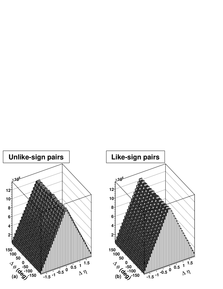
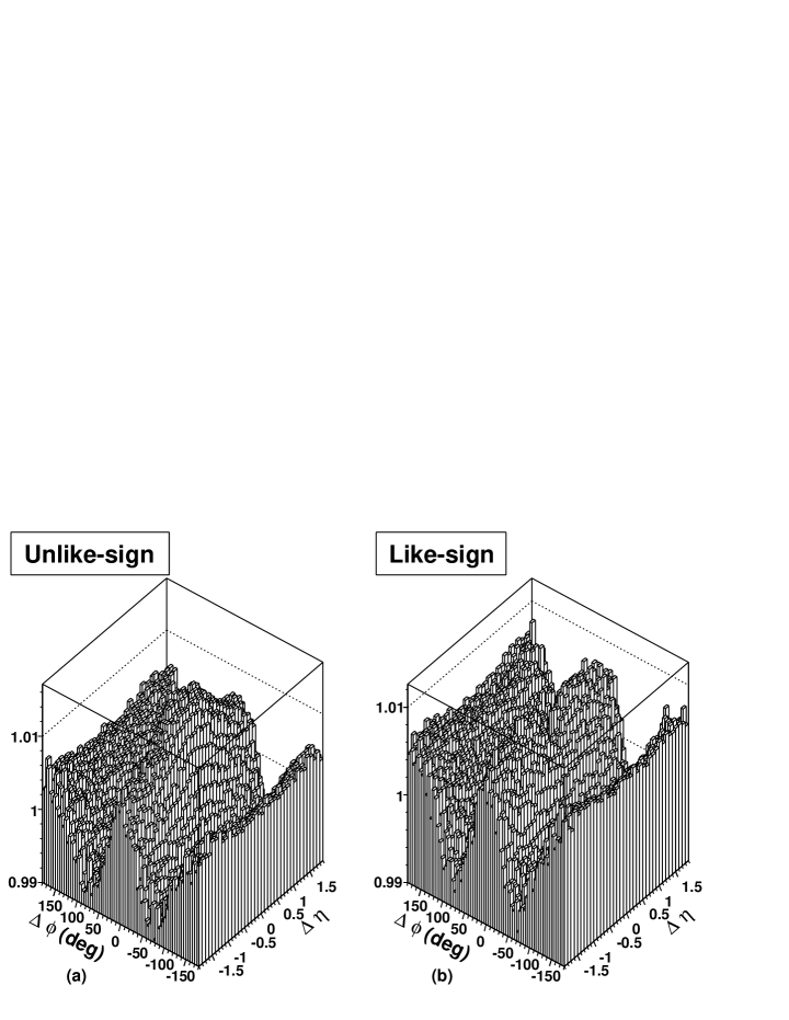
Separate $\Delta\phi$ - $\Delta\eta$ histograms were made for unlike-sign charge pairs and like-sign charge pairs from the same-event-pairs, since their characteristics were different. Both histograms are needed to later determine the CD and the CI correlations as defined in Sections IV A and B. These data are shown in Fig. 1. Similar histograms were made with each track paired with tracks from a different event (mixed-event-pairs), adjacent in time, from the same z vertex bin. This allows the usual technique of dividing the histograms of the same-events-pairs by the histograms of the mixed-events-pairs which strongly suppresses instrumental effects such as acceptance etc., but leaves small residual effects. These include those due to time dependent efficiency of the tracking in the readout boundary regions between the 12 TPC sectors, which had small variations in space charge from event to event. Also space charge in general can cause track distortion and efficiency variation event by event. The ratio of same-event-pairs to mixed-event-pairs histograms is shown in Fig. 2 where the plot was normalized to a mean of 1.

The expected symmetries in the data existed which allowed us to fold all four $\Delta\phi$ - $\Delta\eta$ quadrants into the one quadrant where both $\Delta\phi$ and $\Delta\eta$ were positive. After the cuts described in subsection C, we compared the unfolded bins to the folded average for unlike-sign charge pairs and like-sign charge pairs separately. The $\chi^{2}$ were less than the Degrees of Freedom (DOF), and the $\chi^{2}$ /DOF were within 2-3 $\sigma$ of 1.

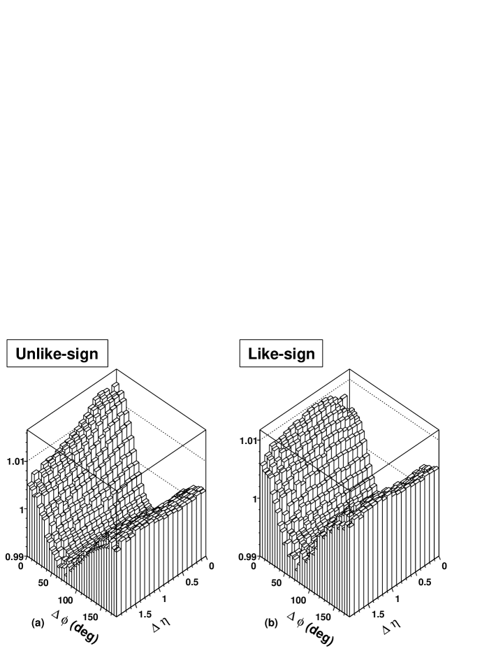
Thus though we searched carefully in a number of ways to find asymmetries in the data via extensive $\chi^{2}$ analyses and observation of fit behavior, none of any significance were found. By folding four quadrants into one, we quadrupled the statistics in each bin analyzed. Fig. 3 shows this folded data after cuts (see subsection C) were made to make track merging, Coulomb, and HBT effects negligible. Henceforth the folded and cut data will be used for our fits.

II.3 Cuts

At small $\Delta\phi$ and small $\Delta\eta$ (i.e. small space angles) track merging effects occur. To determine the cuts needed to reduce these effects to a negligible level, we varied small $\Delta\phi$ and small $\Delta\eta$ cuts. Simultaneously the $\chi^{2}$ of an approximate fit to the data using equation (3) + (4) + (5) was studied as a function of the bins included in the fit. With larger cuts the $\chi^{2}$ behaved properly until one or more of the bins cut out was included in the fit. This caused a huge increase in $\chi^{2}$ , revealing that those bin(s) were distorted by merging effects. We confirmed by visual inspection that track merging effects clearly became important in the bins cut-out. The track merging caused a substantial reduction in track recognition efficiency, and supported the quantitative results of our $\chi^{2}$ analysis. The sharp sensitivity of the $\chi^{2}$ to the cuts showed how localized the merging losses were. We adopted these cuts and they are included in the folded data analyzed

For the unlike-sign charge pairs we cut out the data from the regions 0.0 $<\Delta\eta<$ 0.1 when $0^{\circ}<\Delta\phi<20^{\circ}$ , and 0.1 $<\Delta\eta<$ 0.2 when $0^{\circ}<\Delta\phi<10^{\circ}$ . These cuts to make track merging effects negligible also made the Coulomb effect negligible, since it is effective within a $\Delta$ p of 30 MeV $/c$ . This corresponds to a $2^{\circ}$ opening angle at $p_{t}$ of 0.8 GeV/c. The $2^{\circ}$ along the beam axis near $90^{\circ}$ corresponds to a $\Delta\eta$ of 0.035.

For the like-sign charge pairs we cut out the data from the region 0.0 $<\Delta\eta<$ 0.2 when $0^{\circ}<\Delta\phi<5^{\circ}$ . The HBT effect is already small because of track merging within a $\Delta$ p of 50 MeV/c, corresponding to a $4^{\circ}$ opening angle at 0.8 GeV/c. The $4^{\circ}$ along the beam corresponds to a $\Delta\eta$ of 0.07. All the cuts described above were applied to the mixed events also. Thus the final track merging cuts selected reduce the tracking problems due to overlap and merging to negligible levels, and also reduce Coulomb and HBT effects to negligible levels.

The fits to the subsequently shown data were made over the whole $\Delta\phi$ range. The data for $|\Delta\eta|>1.5$ were cut out, since the statistics were low (see Fig. 1) and tracking efficiency varies at higher $|\Delta\eta|$ .

III Parameterization of data.

We want to obtain a set of functions which will fit the data well, and are interpretable, to the extent practical. We utilized parameterizations representing known, expected physics, or attributable to instrumentation effects. Any remaining terms required to obtain good fits to the data can be considered as signals of new physical effects. Thus signal $\equiv$ data - (known and expected) effects. The three known effects: elliptic flow, residual instrumental effects, momentum and charge conservation terms were parameterized. We then find parameters for the signal terms which are necessary in order to achieve a good fit to our high statistical precision data.

In the following we discuss the relative importance of the effects which are determined by $\chi^{2}$ in our final overall fit to equation (3) + (4) + (5).

III.1 Elliptic Flow

Elliptic flow is a significant contributor to two-particle correlations in heavy ion collisions, and must be accounted for in our analysis. Elliptic flow is not a significant contributor to two-particle correlations in p p collisions. The elliptic flow for STAR Au + Au data has been investigated in an extensive series of measurements and analyses flow using four particle cumulant methods and two particle correlations. This determines a range of amplitudes( $v_{2}$ ) for $\cos$ (2 $\Delta\phi$ ) terms between the four particle cumulant which is the lower flow range boundary of $v_{2}$ ( $v_{2}$ =0.035), and the average value of the four and two particle cumulant which is the upper range boundary of $v_{2}$ ( $v_{2}$ =0.047). These results were determined for the $p_{t}$ range 0.8 to 2 GeV/c by weighting the central trigger spectrum as a function of multiplicity and centrality compared to the minimum bias trigger data for which the $v_{2}$ was measured.

The constraint is used in the following way. We find our best fit to the data by allowing the parameters in the fit to vary freely until the $\chi^{2}$ is minimized. However, there is in the case of the $v_{2}$ parameter a constraint that it must lie in the flow range cited above. Since our best fit was consistent with the bottom of the flow range it was not affected by the constraint. The value of $v_{2}$ cannot be varied to lower values because of the constraint and thus our best fit corresponds to the lower boundary of the flow range and had a $v_{2}$ of 0.035. However, $v_{2}$ can be varied to higher values until either we reach the upper boundary or the fit worsens by $1\sigma$ which is a $\chi^{2}$ change of 32. As discussed in Section VI, our fit worsens by $1\sigma$ when $v_{2}$ is increased to 0.042 well within the flow range 0.035 to 0.047. This represents a systematic error due to flow and is the dominant error( see Section VI ). In Appendix A, a detailed description of multi-parameter fitting and error range determinations are given.

III.2 Instrumental Effects

In addition to the tracking losses resulting from overlapping tracks in the TPC, which we handled by cuts, there are tracks lost in the boundary areas of the TPC between the 12 sectors. These regions result in a loss of acceptance in the $\phi$ measurements since the particle tracks cannot be readout by electronics. This produces a $\phi$ dependence with a period of $30^{\circ}$ which is greatly reduced from about a 4% amplitude to about 0.02% (reduction by a factor of 200), by the normalization to mixed-event-pairs. However it is not completely eliminated, since STAR still has small time dependent variations from event to event, such as space charge effects and slight differences in detector and beam behavior. To correct for the residual readout $\Delta\phi$ dependence, a term with a $30^{\circ}$ period to represent the TPC boundary periodicity and a first harmonic term with a $60^{\circ}$ period were used. The unlike-sign and like-sign charge pairs behave differently over the TPC boundary regions in $\phi$ , because positive tracks are rotated in one direction and negative tracks are rotated in the opposite direction. This requires that the sector terms have an independent phase associated with each. In the Tables I and II the terms are labeled “sector” and “sector2”, “phase” and “phase2”. The functional form for these sector effects is:

\rm Sectors\it(\Delta\phi)=S\sin(12\Delta\phi-\varphi)+S_{2}\sin(6\Delta\phi-\varphi_{2})

(1)

There is a $\phi$ independent effect which we attribute to losses in the larger $\eta$ tracking in the TPC. We utilized mixed-event-pairs with a similar $z$ -vertex to take into account these losses. Imperfections in this procedure leave a small bump near $\Delta\eta$ = 1.15 to be represented in the fit by the terms labeled etabump amp and etabump width in the tables. The width of this bump should be independent of the charge of the tracks, so we constrained it to be the same for like and unlike-sign charge pairs to improve the fit stability. Thus the functional form for this instrumental effect is:

\rm Etabump\it(\Delta\eta)=Ee^{-(\Delta\eta-1.15)^{2}/2\sigma_{E}^{2}}

(2)

In our final $3\sigma$ fits for the combined like and unlike-sign charge pairs (See Tables I and II), leaving out the instrumental corrections would cause our $3\sigma$ fit to deteriorate to a $16\sigma$ fit which is unacceptable. It should be noted that standard $\chi^{2}$ analyses are often not considered credible if the fit exceeds 2-3 $\sigma$ statistical significance.

III.3 Correlations associated with Momentum and Charge Conservation

It is important to ensure that momentum and charge conservation correlation requirements are satisfied. For random emission of single particles with transverse momentum conservation globally imposed, a negative $\cos$ ( $\Delta\phi$ ) term alone can represent this effect. However, the complex correlations that occur at RHIC result in multiple uncorrelated sources which are presently not understood. It was not possible to fit our data with the $\cos$ ( $\Delta\phi$ ) term alone. This fit was rejected by $100\sigma$ . This was not surprising since random emission of single particles with momentum conservation would not lead to the particle correlations observed at RHIC. Therefore we suspected that a more complete description of the momentum and charge conservation was required. No one has succeeded in solving this complex problem in closed form even in the theoretical case where you observe all particles. Hence a reasonable approach was to try to solve it for the tracks we are observing in order to obtain a good fit. We used Fourier expansion in the two variables we have, namely $\Delta\phi$ and $\Delta\eta$ .

Assuming that the $\cos$ ( $\Delta\phi$ ) term for random single particle emission was the first term in a Fourier expansion of odd terms, a second term $\cos$ (3 $\Delta\phi$ ) was added and found to account for about 95% of the $100\sigma$ rejection. Based on the residual analysis we concluded the remaining 5% required $\Delta\eta$ dependent terms for its removal. Therefore we multiplied terms of the type $\cos$ ( $\Delta\phi$ ) and $\cos$ (3 $\Delta\phi$ ) by a $\Delta\eta$ dependent polynomial expansion cutting off at $\Delta\eta^{2}$ . This essentially removed the remaining 5% rejection.

Some of the $\Delta\eta$ dependent terms make quite small contributions in the fits, but in the aggregate they improve our overall fit by about $4\sigma$ . Thus a good fit of $3\sigma$ is downgraded to an unacceptable one of $7\sigma$ without the $\Delta\eta$ dependent expansion, since they add. One should note that fits which exceed $3\sigma$ are often not considered credible by experienced practitioners of precision data analysis, and a precision data analysis was a prime objection of this paper. In addition we found that we needed an overall $\Delta\eta^{2}$ dependent fit parameter.

If we take the sum of the terms we have in the above subsections A, B and C we obtain

	$\displaystyle\bf Bk\it=\rm(Known\it+\rm Expected)Effects\it=$
	$\displaystyle B_{00}+B_{02}\Delta\eta^{2}+B_{10}\cos\Delta\phi+B_{11}\Delta\eta\cos\Delta\phi$
	$\displaystyle+B_{12}\Delta\eta^{2}\cos\Delta\phi+2v_{2}^{2}\cos(2\Delta\phi)+B_{30}\cos(3\Delta\phi)$
	$\displaystyle+B_{31}\Delta\eta\cos(3\Delta\phi)+B_{32}\Delta\eta^{2}\cos(3\Delta\phi)$
	$\displaystyle+\rm Sectors\it(\Delta\phi)+\rm Etabump\it(\Delta\eta)$

Name	Value
lump amplitude ( $A_{u}$ )	0.02426 ${}^{-0.00498}_{+0.00048}$
lump $\Delta\phi$ width ( $\sigma_{\Delta\phi}$ )	32.68 ${}^{-2.12}_{+0.79}$
lump $\Delta\eta$ width ( $\sigma_{\Delta\eta}$ )	1.058 ${}^{-0.137}_{+0.065}$
fourth (f)	0.100 ${}^{+0.031}_{-0.028}$
constant ( $B_{00}$ )	0.99497 ${}^{+0.00142}_{-0.00021}$
$\Delta\eta^{2}$ ( $B_{02}$ )	0.00078 $\mp 0.00018$
$\cos\Delta\phi$ ( $B_{10}$ )	-0.00710 ${}^{+0.00230}_{-0.00035}$
$\Delta\eta\cos\Delta\phi$ ( $B_{11}$ )	0.00092 $\mp 0.00078$
$\Delta\eta^{2}\cos\Delta\phi$ ( $B_{12}$ )	-0.00049 $\mp 0.00057$
$\cos 3\Delta\phi$ ( $B_{30}$ )	0.00058 ${}^{+0.00028}_{-0.00020}$
$\Delta\eta\cos 3\Delta\phi$ ( $B_{31}$ )	0.00030 $\pm 0.00062$
$\Delta\eta^{2}\cos 3\Delta\phi$ ( $B_{32}$ )	-0.00014 $\mp 0.00044$
sector (S)	0.00016 $\pm 0.00006$
phase ( $\varphi$ )	8.6 $\pm 2.1$
sector2 ( $S_{2}$ )	0.00006 $\pm 0.00007$
phase2 ( $\varphi_{2}$ )	23.0 $\pm 10.0$
$\Delta\eta$ bump amp (E)	0.00030 $\mp 0.00025$
$\Delta\eta$ bump width ( $\sigma_{E}$ )	0.189 (fixed)
$\chi^{2}/DOF$	572 / 517

Table 1: Unlike-Sign Charge Pairs Fit Parameters for equation (3) + equation (4). The table has 3 sections. The top section lists parameter names, values and errors for the Approximate Gaussian Signal fit (lump). Fourth(f) is the additional term in the exponent. The source of the above is Subsection III E. The upper error is the change in each parameter when one increases the elliptic flow until the fit is

1\sigma

worse. The lower error is determined by varying each parameter at the lower range of the elliptic flow while all the other parameters are free to readjust until the fit loses

1\sigma

in significance. The middle section has the normalization and a small background term followed by six Momentum and Charge Conservation terms. Source is Subsection III C. The bottom section has instrumental terms. Four terms which are due to TPC sector gaps and two due to large

\eta

tracking errors. Source is Subsection III B. Uncertainties are dominantly systematic, assessed as described in Appendix A.

Name	Value
lump amplitude ( $A_{l}$ )	0.01823 ${}^{-0.00482}_{+0.00069}$
lump $\Delta\phi$ width ( $\sigma_{\Delta\phi l}$ )	32.02 ${}^{-2.91}_{+1.02}$
lump $\Delta\eta$ width ( $\sigma_{\Delta\eta l}$ )	1.847 ${}^{-0.315}_{+0.220}$
dip amplitude ( $A_{d}$ )	-0.00451 ${}^{-0.00092}_{+0.00090}$
dip $\Delta\phi$ width ( $\sigma_{\Delta\phi d}$ )	14.23 ${}^{-2.64}_{+2.91}$
dip $\Delta\eta$ width ( $\sigma_{\Delta\eta d}$ )	0.228 ${}^{+0.050}_{-0.041}$
constant ( $B_{00}$ )	0.99581 ${}^{+0.00136}_{-0.00019}$
$\Delta\eta^{2}$ ( $B_{02}$ )	0.00100 $\mp.00017$
$\cos\Delta\phi$ ( $B_{10}$ )	-0.00737 ${}^{-0.00221}_{-0.00040}$
$\Delta\eta\cos\Delta\phi$ ( $B_{11}$ )	0.00075 ${}^{+0.00072}_{-0.00073}$
$\Delta\eta^{2}\cos\Delta\phi$ ( $B_{12}$ )	-0.00015 ${}^{-0.00054}_{+0.00055}$
$\cos 3\Delta\phi$ ( $B_{30}$ )	0.00070 ${}^{+0.00033}_{-0.00020}$
$\Delta\eta\cos 3\Delta\phi$ ( $B_{31}$ )	-0.00027 ${}^{-0.00064}_{+0.00065}$
$\Delta\eta^{2}\cos 3\Delta\phi$ ( $B_{32}$ )	0.00026 ${}^{+0.00044}_{-0.00045}$
sector (S)	0.00021 $\pm 0.00006$
phase ( $\varphi$ )	22.6 $\mp 1.5$
sector2 ( $S_{2}$ )	0.00007 $\pm 0.00007$
phase2 ( $\varphi_{2}$ )	32.8 $\mp 7.0$
$\Delta\eta$ bump amp (E)	0.00022 ${}^{+0.00024}_{-0.00022}$
$\Delta\eta$ bump width ( $\sigma_{E}$ )	0.189 (fixed)
$\chi^{2}/DOF$	588 / 519

Table 2: Like-Sign Charge Pairs Fit Parameters for equation (3) + equation (4). The table has 3 sections. The top section lists parameter names, values and errors for the Primary Gaussian Signal fit (lump). This is followed by a much smaller Gaussian (dip). Source is Subsection III E. The upper error is the change in each parameter when one increases the elliptic flow until the fit is

1\sigma

worse. The lower error is determined by varying each parameter at the lower range of the elliptic flow while all the other parameters are free to readjust until the fit loses

1\sigma

in significance. The middle section has the normalization and a small background term, followed by six Momentum and Charge Conservation terms. Source is Subsection III C. The bottom section has instrumental terms. Four terms which are due to TPC sector gaps and two due to large

\eta

tracking errors. Source is Subsection III B. Uncertainties are dominantly systematic, assessed as described in Appendix A.

III.4 Fitting with Bk

We used the well known result probability that for a large number of degrees of freedom (DOF), where the number of parameters is a small fraction of DOF and the statistics are high, the $\chi^{2}$ distribution is normally distributed about the DOF. The significance of the fit decreases by $1\sigma$ whenever the $\chi^{2}$ increase is equal to $\sqrt{2(DOF)}$ which for our 517-519 DOF is equal to 32. Appendix A gives further details.

If we fit the functional form of Bk (equation (3)) to both the unlike-sign charge pairs and the like-sign charge pairs, i.e. the whole data set, $\chi^{2}$ is about 10,400 for about 1045 degrees of freedom.

The standard deviation on 1045 DOF is about 46 so the fit is rejected by around $200\sigma$ . We used many free parameters (15) in equation (3) yet additional unknown terms appear to be so sharply varying that it is clearly impossible for the Bk functional form to fit the data. A more detailed discussion of the statistical methods used in the data analyses, and the treatment of systematic and other errors in this paper is given in Appendix A.

III.5 Signal Terms

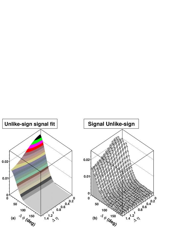
Many signal terms in physics are gaussian-like. We therefore tried fitting the signal data using two dimensional (2-D) gaussians or approximate gaussians. The unlike-sign charge pairs correlations were well fit ( $2\sigma$ ), by adding to Bk an additional 2-D approximate gaussian in $\Delta\eta$ and $\Delta\phi$ (Fig. 4a) given by:

\rm Unlike-sign\>Signal\it=A_{u}e^{-(\Delta\phi^{2}/2\sigma_{\phi}^{2}+\Delta\eta^{2}/2\sigma_{\eta}^{2}-f\Delta\eta^{4})}

(4)

Considering the enormous improvement in fit quality afforded by the addition of this signal term, we conclude that this function in equation (4) provides a compact analytic description of the signal component of the unlike-sign charged pairs correlation data. The fit was improved by the addition of a term dependent on ( $\Delta\eta^{4}$ ) in the exponent (called “fourth” in Table I). The fit for the unlike-sign charge pairs signal data is shown in Fig. 4a. The unlike-sign charge pairs signal data corresponding to the fit (unlike-sign charge pairs data minus Bk ) is shown in Fig. 4b.

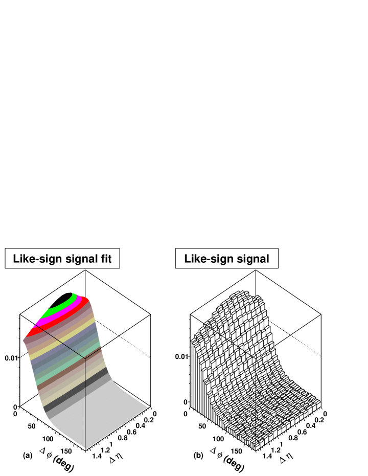
The like-sign charge pairs data which also could not be fit by Bk alone, was well described ( $2\sigma$ ) when we added (see Fig. 3b) a positive 2-D gaussian and a small negative 2-D gaussian dip given by:

	$\displaystyle\rm Like-sign\>Signal\it=A_{l}e^{-(\Delta\phi^{2}/2\sigma_{\phi l}^{2}+\Delta\eta^{2}/2\sigma_{\eta l}^{2})}$
	$\displaystyle+A_{d}e^{-(\Delta\phi^{2}/2\sigma_{\phi d}^{2}+\Delta\eta^{2}/2\sigma_{\eta d}^{2})}$		(5)

Therefore, we conclude that equation (5) provides an efficient description of the signal component of the like-sign charge pairs data. The large signal referred to in Table II as “lump” in the like-sign charge pairs correlation is a 2-D gaussian centered at the origin. It is accompanied by a small narrower 2-D gaussian “dip” (also centered at the origin) subtracted from it. The terms are labeled in the fits as: lump amplitude, dip amplitude, lump $\Delta\phi$ width, lump $\Delta\eta$ width, dip $\Delta\phi$ width, and dip $\Delta\eta$ width. Note that the volume of the dip is about 1.6% of the volume of the large lump signal. However, if we neglected to include this small dip, our fit deteriorates by $28\sigma$ . This dip might be caused by suppression of like-sign charge particle pair emission from localized neutral sources such as gluons. The function fit to the like-sign charged pairs signal data is shown in Fig. 5a. The like-sign charge pairs signal data (like-sign charge pairs data minus Bk) is shown in Fig. 5b. The uncertainties quoted throughout this paper corresponds to a change in $\chi^{2}$ of $\Delta\chi^{2}=32$ , rather than the more commonly used $\Delta\chi^{2}=1$ (see Appendix A for more details).

III.6 Summary of Parameterizations

Equation (3) + (4) yields a $2\sigma$ fit for the unlike-sign charge pairs correlation, and thus is an appropriate and sufficient parameter set.

Equation (3) + (5) yields a $2\sigma$ fit for the like-sign charge pairs correlation, and thus is an appropriate and sufficient parameter set.

Equation (3) + (4) + (5) yields a $3\sigma$ fit for the entire data set, unlike-sign charge pairs correlation + like-sign charge pairs correlation, and thus is an appropriate and sufficient parameter set for the entire data set.

The complex multi dimensional $\chi^{2}$ surface makes the $\chi^{2}$ increase non linearly with the number of error ranges ( $1\sigma$ ) given in the Tables I and II. Therefore, in order to determine the significance of a parameter or group of parameters one must fit without them, and determine by how many $\sigma$ the fit has worsened. Then one uses the normal distribution curve to determine the significance of the omitted parameter(s). The results of such an investigation were:

1.

Leave out $cos(3\Delta\phi)$ and the fit worsens by $95\sigma$ .
2.

Leave out dip and the fit worsens by $28\sigma$ .
3.

Leave out Sector terms and the fit worsens by $11.7\sigma$ .
4.

Leave out $\eta$ dependent $cos(\Delta\phi)$ and $cos(3\Delta\phi)$ terms and the fit worsens by $4.3\sigma$ .
5.

Leave out $\eta$ bump terms and the fit worsens by $1.54\sigma$ .
6.

Leave out sector 2 and the fit worsens by $1.41\sigma$ .

Since our global fit with all the above terms is at the $3\sigma$ level, we conclude that the above terms are necessary. The huge number of $\sigma$ we get for some of the parameters(s) are only to be taken as a qualitative indication of the need for the parameter(s) to fit our high precision data. Due to the uncertainties in determining the number of $\sigma$ far out on the tails of the normal distribution (i.e. $>10\sigma$ ), a quantitative interpretation of them cannot be made.

IV CD and CI Signals

IV.1 Charge Dependent (CD) Signal

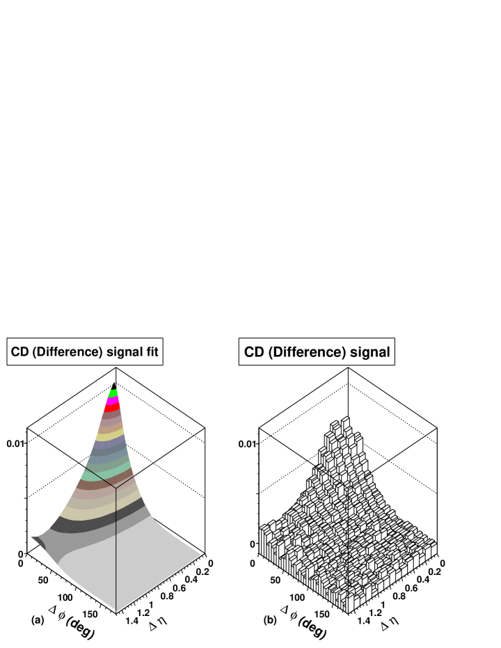
If we subtract the entire like-sign charge pairs correlation (equation (5)) from the unlike-sign charge pairs correlation (equation (4)) we obtain the CD correlation. However it is observed that the background (Bk) of the two terms are close enough in value to cancel each other in the subtraction. Thus the CD signal is essentially the same as the entire CD correlation. In the extensively studied balance function balfun for the correlation due to unlike-sign charge pairs which are emitted from the same space and time region, it is argued that the emission correlation of these pairs can be approximately estimated from the balance function. The balance function for these charged pairs is proportional to the unlike-sign charge pairs minus the like-sign charge pairs. Therefore, the CD signal which is approximately equal to the CD correlation is a qualitative measure of the emission correlation of unlike-sign charge pairs emitted from the same space and time region. In addition to the approximations involved in the balance function, there is the modification to the CD signal discussed in Section IV D.

Fig. 6a shows the fit to the CD signal. Fig. 6b shows the CD signal data that was fit. The signal form is a simple gaussian in both $\Delta\phi$ and $\Delta\eta$ . The gaussian width in $\Delta\phi$ is $28.3^{\circ}\pm 3.4^{\circ}$ (0.49 $\pm$ 0.059 rad) and the gaussian $\Delta\eta$ width is 0.485 $\pm$ 0.054. Converting this pseudo-rapidity to a $\theta$ angle yields a width of $26.7^{\circ}\pm 3.0^{\circ}$ (0.47 $\pm$ 0.052 rad). This correlation has the same angular range in $\Delta\eta$ and $\Delta\phi$ . Therefore we observe pairs of opposite charged particles emitted randomly in the $\eta$ and $\phi$ direction with a correlation which has an average gaussian width of about $27.5^{\circ}\pm 3.2^{\circ}$ (0.48 $\pm$ 0.056 rad) in the $\theta$ angle corresponding to $\Delta\eta$ and also in the azimuth $\Delta\phi$ .

IV.2 Charge Independent (CI) Signal

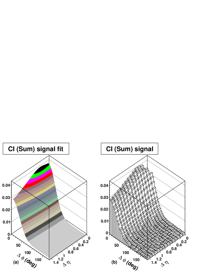
If we add the like-sign charge pairs signal to the unlike-sign charge pairs signal, we obtain the CI signal. The CI signal fit shown in Fig. 7a displays the average structure of the correlated emitting sources. Fig. 7b shows the CI signal data which was fit by the analytic distribution shown in Fig. 7a.

In order to get a good fit to the shape, both in $\Delta\eta$ and $\Delta\phi$ , we needed a more complicated form than one simple 2-D gaussian. The CI signal actually contains an approximate gaussian from the unlike-sign charge pairs signal plus two gaussians from the like-sign charge pairs signal.

We want to obtain a measure of the effective $\Delta\phi$ and $\Delta\eta$ widths of the overall pattern of the CI signal. A good method for doing this is to compare the CI signal with a single gaussian which yields the same root mean square (RMS) values as the actual good fit described above involving two gaussians and an approximate gaussian. For $\Delta\phi$ that $\sigma$ is $32.0^{\circ}\pm 0.6^{\circ}$ (0.56 $\pm$ 0.01 rad). For $\Delta\eta$ that $\sigma$ is 1.55 corresponding to an angle of $66.0^{\circ+1.0^{\circ}}_{-0.6^{\circ}}$ (1.15 $\pm$ 0.02 rad). Thus the correlation is about twice as wide in $\Delta\theta$ , the angle corresponding to $\Delta\eta$ , than in the angle corresponding to $\Delta\phi$ (see Fig. 7a).

Another STAR measurement reports CD and CI correlations at $\sqrt{s_{NN}}$ = 130 GeV/c aya .²²2The CD correlation in Ref. aya is defined as like-sign pairs minus unlike-sign charge pairs which has opposite algebraic sign relative to the definition used in this paper. The major differences between that previous analysis and the present work are the larger range in $p_{t}$ $0.15<p_{t}<2.0$ GeV/c and the lower statistical quality of the limited 130 GeV/c dataset. Although the analysis in Ref. aya included low $p_{t}$ particles there is reasonable qualitative agreement with the present results.

IV.3 Resonance Contribution

To determine the maximum contribution and effect resonances can have on the CI signal we consider the following. Resonances mainly decay into two particles. Therefore, neutral resonances which decay into charged pairs could be a partial source of the unlike-sign charge pairs in CD and CI signals. However, resonances do not add significant correlation to the like-sign charged pairs in either the CD or the CI signals.

We expect that the final state particles from the resonance decay distribution will be symmetrical in the $\Delta\phi$ angle and the angle corresponding to $\Delta\eta$ since we do not expect any polarization mechanism that would disturb this expected symmetry. The fact that in the CD both the $\Delta\phi$ angle and the angle corresponding to $\Delta\eta$ are approximately the same supports this. In this section we are evaluating the possible effects of resonance decay on the CI signal which definitely is observed to be elongated in the corresponding $\Delta\eta$ angle by about a factor of 2 compared to the $\Delta\phi$ angle. The CI signal is always defined as: CI signal = unlike-sign charge pairs signal + like-sign charge pairs signal. CD signal = unlike-sign charge pairs signal - like-sign charge pairs signal. By subtracting the CD signal from the CI signal and rearranging terms in the equation one obtains the following. CI signal = CD signal + 2 $\cdot$ (like-sign charge pairs signal).

There is particular interest in the shape of the CI signal when comparisons are made to theoretical models e.g. HIJING and Ref. themodel . The $\Delta\phi$ shape is about the same in the CI and CD signals. Therefore, we need only estimate the effect of resonances on the $\Delta\eta$ width. By making the extremely unrealistic assumption that the CD signal is composed entirely (100%) of resonances, we can estimate the maximum effect of resonances on the CI signal $\Delta\eta$ width. We use the equivalent gaussian which has the same root mean square (RMS) widths for this calculation. From the data we determine that the $\Delta\eta$ width of the CI signal is increased by a 7% upper limit. However if we use the result from the Appendix B that the resonance content of the CD is 20% or less, we must divide the 7% by 5 which results in an increase of $\Delta\eta$ width of only about 2%. Either estimate of $\Delta\eta$ width increase is inconsequential, compared to the observed approximate factor of two elongation of the $\Delta\eta$ width compared to the $\Delta\phi$ width. Details of these calculations are given in Section VI Systematic Errors and Appendix B.

IV.4 Modification of CI and CD Signals

The CI and CD signals existing at the time of hadronization are changed by the continuing interaction of the particles until kinetic freeze-out, when interactions cease. The interactions are expected to reduce the signals. Therefore we expect that the observed signals are less than those existing at the time of hadronization.

V Net Charge Fluctuation Suppression

Net charge fluctuation suppression is an observed percentage reduction in the RMS width of the distribution of the number of positive tracks minus the negative tracks plotted for each event, compared to the RMS width of a random distribution.

If there are localized, uncharged bubbles of predominantly gluons in a color singlet, when the bubble hadronizes the total charge coming from the bubbles is very close to zero. Therefore if we are detecting an appreciable sample of such bubbles, we expect to see net charge fluctuation suppression.

It should be noted that net charge fluctuation suppression can be deduced from the CD correlation given previously. Net charge fluctuation suppression previously analyzed at lower momenta has been found consistent with resonance decay claude . However the present analysis has different characteristics. Furthermore Ref.themodel has made specific estimates for net charge fluctuation suppression applicable to this experiment. We performed a charge difference analysis for tracks within cuts of $0.8<p_{t}<2.0$ GeV/c and $|\eta|<0.75$ . This would allow a comparison with Ref. themodel .

For each event we determined the difference of the positive tracks minus the negative tracks in our cuts. There was a net mean positive charge of 4.68 $\pm$ 0.009. The width of the charge difference distribution given by (RMS) was $11.149\pm 0.017$ . To determine the net charge fluctuation suppression we need to compare this width with the width of the appropriate random distribution, which would have no net charge fluctuation suppression. However we must arrange a slight bias toward a positive charge so that we end up with the same net mean positive charge as observed. If we now assign a random charge to each track with a slight bias toward being positive such that the mean net charge is also $4.68\pm 0.009$ , the width (RMS) becomes 11.865 $\pm$ 0.017. The percentage difference in the widths which measures the net charge fluctuation suppression is $6.0\%\pm 0.2\%$ .

VI Systematic Errors

Systematic errors were minimized using cuts and corrections. The cuts (see Section II C) were large enough to make contributions from track merging, Coulomb, and HBT effects negligible.

Systematic checks utilized $\chi^{2}$ analyses which verified that the experimental results did not depend on the magnetic field direction, the vertex z coordinate, or the folding procedures (see Sections II A and B). By cutting the track $\eta$ at 1.0 we keep the systematic errors of the track angles below about $1^{\circ}$ backbegone .

In Section IV C we referred to a simulation in Ref. themodel , which estimated that the background resonance contribution to the CD correlation cannot be more than 20% (see Appendix B). From the resonance calculations discussed in Appendix B the background resonance contribution to the unlike-sign charge pairs correlation would be reduced to 5%. The details that justify this are: Our analyses measured an average of 19 unlike-sign charge signal pairs per event from the CD correlation signal. The total average number of unlike-sign charge signal pairs is 88. Therefore with the extreme assumption that all of the CD correlation signal is due to background resonances, 21.6% of the unlike-sign charge signal pairs are due to resonances. However as discussed in Appendix B the estimated contribution of resonances to the CD correlation is 20% or less. Therefore 21.6%/5 = 4.3% is the resonance content of the unlike-sign charge signal pairs, which we rounded to 5%.

We also concluded via an upper limit calculation with the above extremely unrealistic assumption that the shape of the CI signal could only have the measured width in $\Delta\eta$ increased by about 7%. This is inconsequential compared to the factor of two increase in $\Delta\eta$ width compared to $\Delta\phi$ width. For the simulation discussed above, in which resonance backgrounds contribute 20% to the CD correlation, the increase in the CI correlation $\Delta\eta$ width would be limited to about 2%.

The CI signal and the CD signal are more physically significant than the unlike-sign and like-sign charge pairs signals, since they are physically interpretable. The CI signal fit displays the average structure of the correlated emitting sources (Section IV B). The analysis suggests that the CD signal (Section IV A) is a qualitative representation of the emission correlation of the unlike-sign charge pairs emitted from the same space and time region. Elliptic flow contributions to the like and unlike-sign charge pairs signals are approximately equal and therefore cancel in the CD signal. Thus the CD signal is not affected by uncertainty in the elliptic flow amplitude.

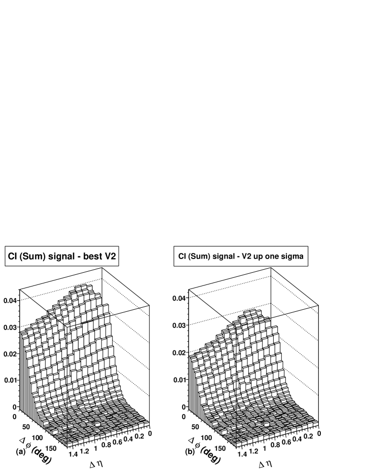
In Fig. 8a we show the CI signal data with the lower flow range value of mean elliptic flow amplitude (weighted over the $p_{t}$ range of the data) used in the fit, namely, $v_{2}$ = 0.035. This is our best fit, in which the value of $v_{2}$ is consistent with the lower flow range. Thus Fig. 8a is the same as Fig. 7b. In Fig. 8b we show the CI signal data with our maximum amount of elliptic flow allowed. This value of elliptic flow causes our fit to be $1\sigma$ worse, and corresponds to a $\chi^{2}$ increase of 32. This results in a mean weighted $v_{2}$ = 0.042. This value of elliptic flow lies in the determined flow range, but is smaller than the upper limit of 0.047 flow . The upper error ranges in Tables I and II are determined by the effect of this change in the elliptic flow (0.042 $>v_{2}>$ 0.035), since it is the dominant error which results in these range values. The main change in Fig. 8b compared to Fig. 8a is that the peak amplitude is reduced by 25%, and the 2 dimensional area is reduced by 34%. However the most significant CI signal parameters in comparing to theoretical models are those that measure the shape, namely the ratio of RMS $\Delta\phi$ and $\Delta\eta$ widths, of a gaussian equivalent to the fit. For our best fit $\Delta\phi$ width = $32.0^{\circ}\pm 0.6^{\circ}$ (0.56 $\pm$ 0.01 rad), and $\Delta\eta$ width = 1.55 which is equivalent to $66.0^{\circ+1.0^{\circ}}_{-0.6^{\circ}}$ (1.15 $\pm$ 0.02 rad). The ratio $\Delta\eta$ equivalent angle/ $\Delta\phi$ = 2.06. For the case of the maximum elliptic flow value the determined widths were $\Delta\phi$ = $30.1^{\circ}$ (0.53 rad), and $\Delta\eta$ = 1.375 ( $61.6^{\circ}$ or 1.08 rad). The ratio $\Delta\eta$ / $\Delta\phi$ = 2.05. Thus the important shape ratio has changed about 1%.

Let us now address the errors due to contamination by including secondary particles arising from weak decays and the interaction of anti-protons and other particles in the beam pipe and material near the beam pipe. These secondary particle backgrounds have been estimated to be about 10-15% starback . In this analysis we are concerned mainly with the angles of the secondary particles relative to the primaries that survive our high $p_{t}$ cut, not their identity or exact momentum magnitude. Our correlations almost entirely depend on angular measurements of $\Delta\phi$ and $\Delta\eta$ . In the range $0.8<p_{t}<2.0$ GeV/c we have considered the behavior of weakly decaying particles and other non-primary particles which could satisfy our distance of closest approach to the primary vertex and $p_{t}$ cuts. Because high $p_{t}$ secondary particles are focused in the same direction as the primaries, only a fraction of these particles have sufficient change in angle that would cause an appreciable error in our correlation. Hence our estimate is a systematic error of about 4% due to secondary particles.

Below we summarize our extensive discussion of systematic errors in this section. Track merging errors, Coulomb, and HBT effects were made negligible by cutting out effected bins at small space angles. Instrumental errors were corrected for in the parameterization. Elliptic flow error is our dominant systematic error, due to the uncertainty that exists in the elliptic flow analyses flow . It should be noted that the size of the upper error range of our parameter errors in Table I and II are determined by the maximum value of the elliptic flow we allowed ( $v_{2}$ =0.042) which corresponds to a $\chi^{2}$ change of 32 ( $1\sigma$ ). The sizeable change to the CI signal shown in Fig. 8b compared to Fig. 8a is due to this maximum allowed value of elliptic flow. As shown above fortunately the shape ratio of the CI signal which is important for theoretical comparison is changed only by about 1%. When more accurate elliptic flow results become available it is a simple matter to insert these in the fits and reduce the resultant error. The next smaller systematic error is due to possible background resonance errors. The smallest systematic error is due to secondary contamination. As discussed above none of these errors affect our important physical conclusions significantly.

VII Discussion

Highly significant correlations are observed for unlike-sign charge pairs and like-sign charge pairs, and consequently for charge dependent (CD) and charge independent (CI) signals. The CD signal is well described (with a $1\sigma$ fit) by a symmetrical 2-D gaussian with an RMS width of about $30^{\circ}$ in both $\Delta\phi$ and $\Delta\eta$ . Conservative simulations in Ref. themodel indicate that the contribution to this CD signal from background resonance decay is less than 20%. Simulations (see Appendix B) estimate that the only significant change due to the background resonances is an increase in the CD amplitude of 20% or less. The CI signal is more complex and is the sum of the unlike-sign charge pairs signal and the like-sign charge pairs signal fits. Therefore it contains an approximate gaussian from the unlike-sign charge pairs signal, and a large positive gaussian plus a small negative gaussian (dip) from the like-sign charge pairs signal. The dip contains only 1.6% of the like-sign charge signal volume. This small dip, observed for the first time, has high significance in the fit. This feature is consistent with what one would expect for suppression of like-sign charge pair emission from a localized neutral source such as gluons.

A 2-D gaussian which yields the same RMS widths as our overall CI signal, has a $\sigma$ along the $\Delta\phi$ direction of $32.0^{\circ}\pm 0.6^{\circ}$ (0.56 $\pm$ 0.01 rad). However the $\Delta\eta$ $\sigma$ is 1.55 corresponding to an angle of approximately $66^{\circ}$ (1.15 rad) and thus is twice as wide.

The mean charge difference for tracks within the chosen analysis cuts is 4.68 $\pm$ 0.009 net positive charges, and the RMS variation of this quantity from event to event is 11.149 $\pm$ 0.017. A random charge assignment constrained to produce the same mean net charge has a larger width of 11.865 $\pm$ 0.017. The difference, $6.0\%\pm 0.2\%$ , measures the net charge fluctuation suppression.

The HIJING model produces jets in our $p_{t}$ range which are nearly symmetrical in $\Delta\phi$ and the angle corresponding to $\Delta\eta$ Wang . The proper way to compare our data with HIJING is to compare our CI signal with the above mentioned HIJING CI correlation from jets. As shown in IV B, our CI signal is highly asymmetric since the angle corresponding to $\Delta\eta$ is about twice the angle $\Delta\phi$ thus strongly contradicting these basic characteristics of HIJING jets correlations.

Ref.PBM presents a detailed comparison of the STAR data presented here with a model based on a ring of localized bubbles emitting charged particles from the central fireball surface at kinetic freeze out. Good consistency with the STAR data presented in the present paper is reportedPBM .

VIII Summary and Conclusions

We performed an experimental investigation of particle-pair correlations in $\Delta\phi$ and $\Delta\eta$ using the main Time Projection Chamber of the STAR detector at RHIC. We investigated central Au + Au collisions at $\sqrt{s_{NN}}$ = 200 GeV, selecting tracks having transverse momenta $0.8<p_{t}<2.0$ GeV/c, and the central pseudo-rapidity region $|\eta|<1.0$ . The data sample consists of 2 million events, and the symmetries of the data in $\Delta\eta$ and $\Delta\phi$ allow four quadrants to be folded into one. The entire data set (unlike-sign charge pairs and like-sign charge pairs) was fit by a reasonably interpretable set of parameters, 17 for the unlike-sign charge pairs and 19 for the like-sign charge pairs. These parameters are small in number compared to the total number of degrees of freedom, which was over 500 for each of the two types of pairs. Every fit reported here using these parameters was a good fit of 2 to 3 $\sigma$ or less.

Section VI discusses systematic errors. From our analysis of the systematic errors we conclude that the important features of our data and the conclusions drawn have not been significantly affected by the systematic errors.

Section VII discusses the results and model fits.

This paper serves as an excellent vehicle for making detailed comparisons with, and testing of various theoretical models such as the Bubble Model themodel and other relevant models.

IX Acknowledgment

We thank the RHIC Operations Group and RCF at BNL, and the NERSC Center at LBNL for their support. This work was supported in part by the Offices of NP and HEP within the U.S. DOE Office of Science; the U.S. NSF; the BMBF of Germany; IN2P3, RA, RPL, and EMN of France; EPSRC of the United Kingdom; FAPESP of Brazil; the Russian Ministry of Science and Technology; the Ministry of Education and the NNSFC of China; IRP and GA of the Czech Republic, FOM of the Netherlands, DAE, DST, and CSIR of the Government of India; Swiss NSF; the Polish State Committee for Scientific Research; SRDA of Slovakia, and the Korea Sci. & Eng. Foundation.

Appendix A Multi-parameter fitting in the large DOF region and systematic uncertainties

Let us now consider the detail of multi-parameter data analysis in the large DOF region in terms of change of $\chi^{2}$ for our 517-519 n for unlike-sign and like-sign charge pairs respectively. A $1\sigma$ change in the significance of the individual fits require the change in $\chi^{2}$ of 32. The reader is referred to Ref.probability from which we quote: “For large n(DOF), the $\chi^{2}$ p.d.f.(probability density function) approaches a gaussian with mean = n and variance( $\sigma$ ) squared = 2n.” For n $>$ 50-100 this result has been considered applicable, and it remains applicable and becomes more accurate as n increases toward infinity. Thus for our 517-519 n, $1\sigma$ = $\sqrt{2n}$ =32.

The statistical significance of any fit in this paper can be obtained by the following procedure: The number of $\sigma$ ’s of fit = ( $\chi^{2}$ - n)/32. The number of $\sigma$ ’s refer to the normal distribution curve.

For large DOF(bins - parameters) fluctuations occur because of the many bins. When one fits the parameters, they will try and describe some of these fluctuations. Therefore we need to check whether the fluctuations in the data sample are large enough to significantly distort the parameter values. This has traditionally been done by using the confidence level tables vs. $\chi^{2}$ which allows a reasonable determination of the fluctuations due to binning. The approximation (described above) we have used is an accurate extension of the confidence level tables.

Let us consider our method of assigning systematic error ranges to the parameters. Our objective is to obtain error ranges which are not likely to be exceeded if future independent data samples taken under similar conditions are obtained by repetition of the experiment by STAR or others. We want to avoid the confusion and uncertainty of apparent significant differences in parameters when the fit to new data does not differ significantly from a previous fit. We allow each parameter, one at a time, to be varied (increased and then decreased) in both directions while all the other parameters are free to readjust until the overall fit $\chi^{2}$ degrades in significance by $1\sigma$ . This corresponds to an increase of $\chi^{2}$ of 32 for the unlike-sign and like-sign charged pairs fits. The $\chi^{2}$ surface has been observed, and $\chi^{2}$ increases very non linearly with small increases of the parameter beyond the error range.

When one assumes that the parameter error is given by a $\chi^{2}$ change of 1 in the best fitstatistics , this is correct for the case where you know the underlying physics. The purpose of our use of parameters is not to determine their true values, since we do not know the underlying physics. We use the parameters to determine an analytic description of the data that fits it within 2-3 $\sigma$ .

Let us address how one determines the significance of a parameter or a particular group of parameters in the case of this multi-parameter analysis. It is entirely incorrect to compare the error ranges in Table I and II with the parameter value. The only correct way to determine the significance of a parameter or group of parameters in the multi-parameter fit is to leave the parameter(s) out of the fit and refit without the parameter(s). One then determines by how many $\sigma$ ’s the overall fit has degraded compared to a change of 32 for $1\sigma$ .

One should note that the upper error range on a parameter in Tables I and II represents the change in value of the parameter as we increase $v_{2}$ , our dominant error, from our best fit until the fit worsens by $1\sigma$ ( $\chi^{2}$ increases by 32). The other parameters are free to readjust during the foregoing variation. The lower error range is the result of changing the parameter in the opposite direction of it in the upper range while the other parameters are free to readjust until the fit decreases in significance by $1\sigma$ . The largest error which dominates the upper systematic error range determination is the variation of the $v_{2}$ error. However the constraint of $v_{2}$ to the flow range, and the fact that our best fit is at the lower end of the range means that flow is not varied when we determine the lower error. Therefore the elimination of the large flow variation leads to generally smaller lower error ranges and thus observed asymmetry between the upper and lower error ranges.

Finally if one fixes any one of the parameters at the end of the error ranges with the correct $v_{2}$ assigned (0.042 upper and 0.035 lower) and lets all the other parameters readjust, one will achieve an overall fit which is only worse by $1\sigma$ (a $\chi^{2}$ increase of 32).

Appendix B resonance calculations

In this section we discuss background resonances which have the following meaning. Background resonances are resonances that only contribute to the unlike-sign charge pair correlation. Any resonance that is emitted as part of a correlated emitter will also have a like-sign charge correlation. This is because any of the charges will have another particle of the same charge to correlate with which is also emitted by the correlated emitter. The background resonances we are discussing are not part of the correlated emitters we want to study, but will add to the CD correlation.

In Ref. themodel a table of resonances and particles was considered in a thermal resonance gas model. The resonance content was adjusted to cause the 20% net charge fluctuation suppression observed at lower momentum in a STAR experiment for central Au + Au collisions. The result of this model calculation is a 20% contribution of resonances to the CD correlation. The $p_{t}$ range of the analysis $0.8<p_{t}<2.0$ GeV/c tends to have the symmetric pairs of particles from resonance production decay into angles within the range of our cuts. However asymmetric decays only contribute one particle of the pair and thus do not add to the correlation. Therefore effectively only a part of the estimated resonance contribution affects the correlation measurement. Our simulations reveal that the only significant change that the background resonance contribution would introduce in the CD correlation is an increase in amplitude of 20% or less. The CI signal = CD signal + 2 $\cdot$ (like-sign charge pairs signal). The resonance contribution to the like-sign charge pairs signal is small. The affect of resonances on the CI signal elongation in the $\Delta\eta$ width is estimated by the model simulation to be a factor five lower than the extreme maximum case previously assumed, that the entire CD correlation is composed of background resonances. Thus this would result in a $\Delta\eta$ width elongation of the CI signal of approximately 2% instead of the upper limit of 7%.

References

(1) STAR Collaboration J. Adams et. al., Nucl. Phys. A 757, 102 (2005).
(2) For an overview see:Quark Matter Formation and Heavy Ion Collisions, Proceedings Biefield Workshop (May 82), Proc. of Quark Matter 2004, J. Phys. G 30, s633-s1392 (2004).
(3) Special Issue: The Relativistic Heavy Ion Collider Project RHIC and its Detectors, Nucl.Instrum. Meth. A 499, pp 235-880 (2003).
(4) J. Adams et al.(STAR Collaboration), Phys. Rev. C 70, 054907 (2004).
(5) F. Karsch, Nucl. Phys. A 698, 199c (2002).
(6) L. Van Hove, Hadronization Quark-Gluon Plasma in Ultra-Relativistic Collisions, CERN-TH (1984) 3924, L. Van Hove, Hadronization Model for Quark-Gluon Plasma in Ultra-Relativistic Collisions, Z. Phys. C27, 135 (1985).
(7) S.J. Lindenbaum and R.S. Longacre, J. Phys. G 26, 937 (2000). This paper contains earlier (85 onward) references by these authors.
(8) S.J. Lindenbaum, R.S. Longacre and M. Kramer Eur. Phys. J. C (Particles and Fields) 30, 241-253 (2003). DOI: 10. 1140/epjc/s2003-01 268-3
(9) J. Adams et al.(STAR Collaboration), Phys. Rev. C 71, 044906 (2005), S. S. Adler et al.(PHENIX collaboration), Phys. Rev. Lett. 93, 152302 (2004).
(10) Nucl. Instrum. Meth. A 499,(2003), C. Adler et al., 433-436, K.H. Ackermann et al.(STAR Collaboration), 624-632, M. Anderson et al., 659-678, F.S. Bieser et al., 766-777.
(11) K.H. Ackerman et al.(STAR Collaboration), Phys. Rev. Lett. 86, 402 (2001). C. Adler et al.(STAR Collaboration), Phys. Rev. Lett. 90, 032301 (2003), J. Adams et al.(STAR Collaboration), Phys. Rev. C72, 014904 (2005).
(12) S. Edelman et al Phys. Lett B 592, (2004), 31. Probability, Section 31.4.4 $\chi^{2}$ distribution, p 278(REVIEW OF PARTICLE PROPERTIES).
(13) S. A. Bass, P. Danielewicz and S. Pratt, Phys. Rev. Lett.85, 2689 (2000), S. Chang et al., Phys. Rev. C69, 54906 (2004), P. Christakoglou, A. Petridis and M. Vassiliou, Nucl. Phys. A749, 279c (2005).
(14) J. Adams et. al.,(STAR Collaboration), Phys. Rev. C 73, 064907 (2006), Phys. Lett. B 634, 347 (2006).
(15) J. Adams et al.(STAR Collaboration), Phys. Rev. C 68, 044905 (2003).
(16) C. Adler et al.(STAR Collaboration), Phys. Rev. Lett. 90, 082302 (2003).
(17) C. Adler et al.(STAR Collaboration), Phys. Rev. Lett. 87, 112303 (2001), J. Adams et al. (STAR Collaboration), Phys. Rev. Lett. 92, 112301 (2004).
(18) X.N. Wang and M. Gyulassy, Phys. Rev. D 44, 3501 (1991).
(19) S.J. Lindenbaum and R.S. Longacre, Eur. Phys. J. C. (Accepted-in press), Parton Bubble Model for Two Particle Angular Correlations at RHIC/LHC.
(20) S. Edelman et al Phys. Lett B 592, (2004), 32.Statistics, p 279(REVIEW OF PARTICLE PROPERTIES).

Δ​ϕ​Δ​ηΔitalic-ϕΔ𝜂\Delta\phi\Delta\eta Correlations in Central Au+Au Collisions at sN​N=subscript𝑠𝑁𝑁absent\sqrt{s_{NN}}= 200 GeV