Computational studies of light acceptance and propagation in straight and curved multimodal active fibres

C P Achenbach¹¹1 Present address: Institut für Kernphysik, Joh. Gutenberg-Universität Mainz, J J Becher-Weg 45, 55099 Mainz, Germany. and J H Cobb University of Oxford, Sub-department of Particle Physics, Denys Wilkinson Building, Keble Road, Oxford OX1 3RH, UK p.achenbach@physics.ox.ac.uk

Abstract

A Monte Carlo simulation has been performed to track light rays in cylindrical multimode fibres by ray optics. The trapping efficiencies for skew and meridional rays in active fibres and distributions of characteristic quantities for all trapped light rays have been calculated. The simulation provides new results for curved fibres, where the analytical expressions are too complex to be solved. The light losses due to sharp bending of fibres are presented as a function of the ratio of curvature to fibre radius and bending angle. It is shown that a radius of curvature to fibre radius ratio of greater than 65 results in a light loss of less than 10% with the loss occurring in a transition region at bending angles $\Phi\sim\pi/8$ rad.

Keywords: Fibre optics, propagation and scattering losses, geometrical optics, wave fronts, ray tracing

1 Introduction

Active optical fibres are becoming more and more important in the field of detection and measurement of ionising radiation and particles. Light is generated inside the fibre either through interaction with the incident radiation (scintillating fibres) or through absorption of primary light (wavelength-shifting fibres). Plastic fibres with large core diameters, i.e. where the wavelength of the light being transmitted is much smaller than the fibre diameter, are commercially available and readily fabricated, have good timing properties and allow a multitude of different geometrical designs. The low costs of plastic materials make it possible for many present day or future experiments to use such fibres in large quantities (see [1] for a review of active fibres in high energy physics). For the construction of the highly segmented tracking detector of the ATLAS experiment approved for the LHC collider at CERN more than 600,000 wavelength-shifting fibres have been used [2]. Our work is also motivated by the fact that spiral fibres embedded in scintillators are being used for calorimetric measurements in long base line neutrino oscillation experiments, most recently in the MINOS experiment [3].

The treatment of small diameter optical fibres involves electromagnetic theory applied to dielectric waveguides, which was first achieved by Snitzer [4] and Kapany et al [5]. Although this approach provides insight into the phenomenon of total internal reflection and eventually leads to results for the field distributions and electromagnetic radiation for curved fibres, it is advantageous to use ray optics for applications to large diameter fibres where the waveguide analysis is an unnecessary complication. In ray optics a light ray may be categorised by its path along the fibre. The path of a meridional ray is confined to a single plane, all other modes of propagation are known as skew rays. The optics of meridional rays in fibres was developed in the 1950s [6] and can be found in numerous textbooks, e.g. in [7, 8, 9]. Since then, the scientific and technological progress in the field of fibre optics has been enormous. Despite the extensive coverage of theory and experiment in this field, only fragmentary studies on the trapping efficiencies and refraction of skew rays in curved multimode fibres could be found [10, 11, 12, 13]. We have therefore performed a three-dimensional simulation of photons propagating in simple circularly curved fibres in order to quantify the losses and to establish the dependence of these losses on the angle of the bend. We have also briefly investigated the time dispersion in fibres. For our calculations a common type of fibre in particle physics is assumed, specified by a polystyrene core of refractive index $n_{\it core}=$ 1.6 and a thin polymethylmethacrylate (PMMA) cladding of refractive index $n_{\it clad}=$ 1.49, where the indices are given at a wavelength of 590 nm. Another common cladding material is fluorinated polymethacrylate with $n_{\it clad}=1.42$ . Typical diameters are in the range of 0.5 – 1.5 mm.

This paper is organised as follows: section 2 describes the analytical expressions of trapping efficiencies for skew and meridional rays in active, i.e. light generating, fibres. The analytical description of skew rays is too complex to be solved for sharply curved fibres and the necessity of a simulation becomes evident. In section 3 a simulation code is outlined that tracks light rays in cylindrical fibres governed by a set of geometrical rules derived from the laws of optics. section 4 presents the results of the simulations. These include distributions of the characteristic properties which describe light rays in straight and curved fibres, where special emphasis is placed on light losses due to the sharp bending of fibres. Light dispersion is briefly reviewed in the light of the results of the simulation. The last section provides a short summary.

2 Trapping of photons

When using scintillating or wavelength-shifting fibres in charged particle detectors the trapped light as a fraction of the intensity of the emitted light is very important in determining the light yield of the system. For very low light intensities as encountered in many particle detectors the photon representation is more appropriate to use than a description by light rays. Whether the fibres are scintillating or wavelength-shifting one is only ever concerned with a few 10’s or 100’s of photons propagating in the fibre and single photon counting is often necessary.

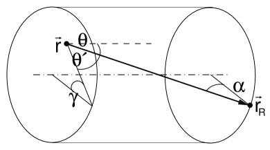
The geometrical path of any rays in optical fibres, including skew rays, was first analysed in a series of papers by Potter [14] and Kapany [15]. The treatment of angular dependencies in our paper is based on that. The angle $\gamma$ is defined as the angle of the projection of the light ray in a plane perpendicular to the axis of the fibre with respect to the normal at the point of reflection. One may describe $\gamma$ as a measure of the ‘skewness’ of a particular ray, since meridional rays have this angle equal to zero. The polar angle, $\theta^{\prime}$ , is defined as the angle of the light ray in a plane containing the fibre axis and the point of reflection with respect to the normal at the point of reflection. It can be shown that the angle of incidence at the walls of the cylinder, $\alpha$ , is given by $\cos{\alpha}=\cos{\theta^{\prime}}\,\cos{\gamma}$ . The values of the two orthogonal angles $\theta^{\prime}$ and $\gamma$ will be preserved independently for a particular photon at every reflection along its path.

In general for any ray to be internally reflected within the cylinder of the fibre, the inequality $\sin{\alpha}\geq\sin{\theta^{\prime}_{\it crit}}=n_{\it clad}/n_{\it core}$ must be fulfilled, where the critical angle, $\theta^{\prime}_{\it crit}$ , is given by the index of refraction of the fibre core, $n_{\it core}$ , and that of the cladding, $n_{\it clad}$ . In the meridional approximation the above equations lead to the well known critical angle condition for the polar angle, $\theta^{\prime}\geq\theta^{\prime}_{\it crit}$ , which describes an acceptance cone of semi-angle, $\theta\ [=\pi/2-\theta^{\prime}]$ , with respect to the fibre axis (see for example [14] and references therein). Thus, in this approximation all light within the forward cone will be considered as trapped and undergo multiple total internal reflections to emerge at the end of the fibre.

For the further discussion in this paper it is convenient to use the axial angle, $\theta$ , as given by the supplement of $\theta^{\prime}$ , and the skew angle, $\gamma$ , to characterise any light ray in terms of its orientation, see figure 1 for an illustration.

The flux transmitted by a fibre is determined by an integration over the angular distribution of the light emitted within the acceptance domain, i.e. the phase space of possible propagation modes. Using the expression given by Potter et al [16] and setting the transmission function, which parameterises the light attenuation, to unity the light flux can be written as follows:

\eqalign{F&=F_{m}+F_{s}\\ &=4\rho^{2}\int_{\theta=0}^{\theta_{\it crit}}\int_{\gamma=0}^{\pi/2}\int_{\phi=0}^{\pi/2}I(\theta,\phi)\,\cos^{2}{\gamma}\,d\gamma\,d\Omega\ +\\ &4\rho^{2}\int_{\theta=\theta_{\it crit}}^{\pi/2}\int_{\gamma=\overline{\gamma}(\theta)}^{\pi/2}\int_{\phi=0}^{\pi/2}I(\theta,\phi)\,\cos^{2}{\gamma}\,d\gamma\,d\Omega\ ,}

(1)

where $d\Omega$ is the element of solid angle, $\overline{\gamma}(\theta)$ refers to the maximum axial angle allowed by the critical angle condition, $\rho$ is the radius of a cylindrical fibre and $I(\theta,\phi)$ is the angular distribution of the emitted light in the fibre core. The two terms, $F_{m}$ and $F_{s}$ , refer to either the meridional or skew cases, respectively. The lower limit of the integral for $F_{s}$ is $\overline{\gamma}=\arccos{(\sin{\theta_{\it crit}}/\sin{\theta})}$ .

The trapping efficiency for forward propagating photons, $\epsilon^{1/2}$ , may be defined as the fraction of totally internally reflected photons. The formal expression for the trapping efficiency, including skew rays, is derived by dividing the transmitted flux by the total flux through the cross-section of the fibre core, $F_{0}$ . For isotropic emission of fluorescence light the total flux equals $4\pi^{2}\rho^{2}I_{0}$ . Then, the first term of equation (1) gives the trapping efficiency in the meridional approximation,

\epsilon^{1/2}_{m}=F_{m}/F_{0}=\frac{1}{2}(1-\cos{\theta_{\it crit}})\approx\frac{\theta^{2}_{\it crit}}{4}\ ,

(2)

where all photons are considered to be trapped if $\theta\leq\theta_{\it crit}$ , independent of their actual skew angles.

The integration of the second term of equation (1) gives the contributions of all skew rays to the trapping efficiency. Integrating by parts, one obtains

\epsilon^{1/2}_{s}=\frac{1}{2}\cos{\theta_{\it crit}}-\frac{\cos^{2}{\theta_{\it crit}}\sin{\theta_{\it crit}}}{2\pi}\int_{0}^{1}\frac{dt}{\sqrt{(1-t)\,t}\,\left(1-t\cos^{2}{\theta_{\it crit}}\right)}\ ,

(3)

with $t=\cos^{2}{\theta}/\cos^{2}{\theta_{\it crit}}$ . Complex integration leads to the result:

\epsilon^{1/2}_{s}=\frac{1}{2}(1-\cos{\theta_{\it crit}})\cos{\theta_{\it crit}}\ .

(4)

The total initial trapping efficiency is then:

\epsilon^{1/2}=\frac{1}{2}(1-\cos^{2}{\theta_{\it crit}})\approx\frac{\theta^{2}_{\it crit}}{2}\ ,

(5)

which is approximately twice the trapping efficiency in the meridional approximation for small critical angles. The trapping efficiency of rays is crucially dependent on the circular symmetry of the core-cladding interface. Any ellipticity or variation in the fibre diameter will lead to the refraction of some skew rays. Furthermore, skew rays have a much longer optical path length, suffer from more reflections and therefore get attenuated more quickly, see section 4 for a quantitative analysis of this effect. In conclusion, for long fibres the effective trapping efficiency is closer to $\epsilon^{1/2}_{m}$ than to $\epsilon^{1/2}$ . Formula 2 yields a trapping efficiency of $\epsilon^{1/2}_{m}=$ 3.44% for plastic fibres with $n_{\it core}=$ 1.6 and $n_{\it clad}=$ 1.49. For these “standard” parameters the efficiency in formula 4 evaluates to $\epsilon^{1/2}_{s}=$ 3.20% and in formula 5 to $\epsilon^{1/2}=$ 6.64%.

3 Description of the tracking code

The aim of the program is to track light rays through a fibred. Since the analytic analysis of the passage of skew rays along a curved fibre is exceedingly complex we treat the problem with a Monte Carlo technique. This type of numerical integration using random numbers is a standard method in the field of particle physics and is now practical given the CPU power currently available. On its path the ray is subject to attenuation, parameterised firstly by an effective absorption coefficient and secondly by a reflection coefficient. At the core-cladding interface the ray can be reflected totally or partially internally. In the latter case a random number is compared to the reflection probability to select reflected rays.

Light rays are randomly generated on the circular cross-section of a fibre with radius $\rho$ . An arbitrary ray is defined by its axial and azimuthal or skew angle. An advantage of this method is that any distribution of light rays can easily be generated. The axis of the fibre is defined by a curve $z=f(s)$ where $s$ is the arc length. For $s<0$ , it is a straight fibre along the negative $z$ -axis and for $0<s<L_{F}$ , the fibre is curved in the $xz$ -plane with a radius of curvature $R_{\it curve}$ . In particular, the curve $f(s)$ is tangential to the $z$ -axis at $s=0$ .

Light rays are represented as lines and determined by two points, $\vec{r}$ and $\vec{r}^{\,\prime}$ . The points of incidence of rays with the core-cladding interface are determined by solving the appropriate systems of algebraic equations. In the case of a straight fibre the geometrical representation of a straight cylinder is used resulting in the quadratic equation

(x+(x^{\prime}-x)\times m)^{2}+(y+(y^{\prime}-y)\times m)^{2}-\rho^{2}=0\ .

(6)

The positive solution for the parameter $m$ defines the point of incidence, $\vec{r}_{R}$ , on the cylinder wall. In the case of a fibre curved in a circular path, the cylinder equation is generalized by the torus equation

\eqalign{(R_{\it curve}-((x+(x^{\prime}-x)\times m+R_{\it curve})^{2}\\ +(z+(z^{\prime}-z)\times m)^{2})^{1/2})^{2}\\ +(y+(y^{\prime}-y)\times m)^{2}-\rho^{2}=0\ .}

(7)

The coefficients of this fourth degree polynomial are real and depend only on $R_{\it curve}$ and the vector components of $\vec{r}$ and $\vec{r}^{\,\prime}$ up to the fourth power. In most cases there are two real roots, one for the core-cladding intersection in the forward direction and one at $\vec{r}$ if the initial point already lies on the cylinder wall. The roots are found using Laguerre’s method [17]. It requires complex arithmetic, even while converging to real roots, and an estimate for the root to be found. The routine implements a stopping criterion in case of non-convergence because of round-off errors. The initial estimate is given by the intersection point of the light ray and a straight cylinder that has been rotated and translated to the previous reflection point. A driver routine is used to apply Laguerre’s method to all four roots and to perform the deflation of the remaining polynomial. Finally the roots are sorted by their real part. The smallest positive, real solution for $m$ is then used to determine the reflection point, $\vec{r}_{R}$ .

After the point of incidence has been found, the reflection length and absorption probability can be calculated. The angle of incidence, $\alpha$ , is given by $\cos{\alpha}=\vec{r}_{in}\cdot\vec{n}$ , where $\vec{n}$ denotes the unit vector normal to the core-cladding interface at the point of reflection and $\vec{r}_{in}=(\vec{r}-\vec{r}_{R})/|\vec{r}-\vec{r}_{R}|$ is the unit incident propagation vector. Now the reflection probability corresponding to this angle $\alpha$ is determined. In case the ray is partially or totally internally reflected the total number of reflections is increased and the unit propagation vector after reflection, $\vec{r}_{\it out}$ , is then calculated by mirroring $\vec{r}_{in}$ with respect to the normal vector: $\vec{r}_{\it out}=\vec{r}_{in}-2\vec{n}\cos{\alpha}$ . The program returns in a loop to the calculation of the next reflection point. When the ray is absorbed on its path or not reflected at the reflection point the next ray is generated at the fibre entrance end. A scheme on the main steps of the program can be found in figure 2. At any point of the ray’s path its axial, azimuthal and skew angle are given by scalar products of the ray vector with the coordinate axes in a projection on a plane perpendicular to the fibre axis and parallel to the fibre axis, respectively. The transmitted flux of a specific fibre, taking all losses caused by bending, absorption and reflections into account, is calculated from the number of lost rays compared to the number of rays reaching the fibre exit end.

This method gives rise to an efficient simulation technique for fibres with constant curvature. It is possible to extend the method for the study of arbitrarily curved fibres by using small segments of constant curvature. In the current version of the program light rays are tracked in the fibre core only and no tracking takes place in the surrounding cladding, corresponding to infinite cladding thickness. In long fibres cladding modes will eventually be lost, but for lengths $<1$ m they can contribute to the transmission function. The simulation code is written in Fortran and it takes about 1.5 ms to track a skew ray through a curved fibre.

4 Results of the tracking code

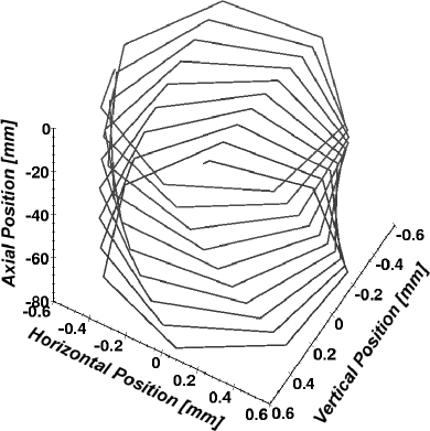
Figure 1 shows the passage of a skew ray along a straight fibre. The light ray has been generated off-axis with an axial angle of $\theta=0.42$ and would not be trapped if it were meridional. In general, the projection of a meridional ray on a plane perpendicular to the fibre axis is a straight line, whereas the projection of a skew ray changes its orientation with every reflection. In the special case of a cylindrical fibre all meridional rays pass through the fibre axis. The figure illustrates the preservation of the skew angle, $\gamma$ , during the propagation.

4.1 Trapping efficiency and acceptance domain

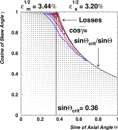
Figure 3(a) shows the total acceptance domain and its splitting into the meridional and skew regions in the meridional ray approximation. The phase space density, i.e. the number of trapped rays per angular interval, is represented by proportional boxes. The density increases with $\cos^{2}{\gamma}$ and $\sin{\theta}$ . The contours relate to sharply curved fibres and are explained in section 4.4. Figure 3(b) shows a projection of the phase space onto the $\sin\theta$ -axis. A peak around the value $\sin{\theta_{\it crit}}$ is apparent. A skew ray can be totally internally reflected at larger angles $\theta$ than meridional rays and the relationship between the minimum permitted skew angle, $\overline{\gamma}$ , at a given axial angle, $\theta$ , is determined by the critical angle condition: $\cos{\overline{\gamma}}=\sin{\theta_{\it crit}}/\sin{\theta}$ .

Photons are generated randomly on the cross-section of the fibre with an isotropic angular distribution in the forward direction. The figure gives values for the two trapping efficiencies which can be determined by integrating over the two angular regions. The integrals are identical in value to the expressions in formulae 2 and 4. It is obvious from the critical angle condition that a photon emitted close to the cladding has a higher probability to be trapped than when emitted close to the centre of the fibre. For a given axial angle the range of possible azimuthal angles, in which the photons are uniformly distributed, for the photon to get trapped increases with the radial position, $\hat{\rho}$ , of the light emitter in the fibre core. It can be deduced from figure 4 that the meridional approximation is a good estimate for $\epsilon$ if the photons originate at radial positions $\hat{\rho}<0.8$ . The trapping of skew rays only becomes significant for photons originating at radial positions $\hat{\rho}\geq 0.9$ . This fact has been discussed before, e.g. in [18]. Figure 4 shows the the trapping efficiency as a function of the axial angle. All photons with axial angles below $\theta_{\it crit}$ are trapped in the fibre, whereas photons with larger angles are trapped only if their skew angle exceeds the minimum permitted skew angle. It can be seen that the trapping efficiency falls off very steeply with the axial angle.

4.2 Propagation of photons

The analysis of trapped photons is based on the total photon path length per axial fibre length, $P$ , the number of internal reflections per axial fibre length, $\eta$ , and the optical path length between successive internal reflections, $l_{R}$ , where we follow the nomenclature of Potter and Kapany. It should be noted that these three variables are not independent as $P=\eta\times l_{R}$ .

Figure 5 shows the distribution of the normalised path length, $P(\theta)$ , for photons reaching the exit end of straight and curved fibres of 0.6 mm radius. The figure also gives results for curved fibres of two different radii of curvature. The distribution of path lengths shorter than the path length for meridional photons propagating at the critical angle is almost flat. It can easily be shown that the normalised path length along a straight fibre is given by the secant of the axial angle and is independent of other fibre dimensions: $P(\theta)=\sec\theta$ . In case of the curved fibre the normalised path length of the trapped photons is less than the secant of the axial angle and photons on near meridional paths are refracted out of the fibre most.

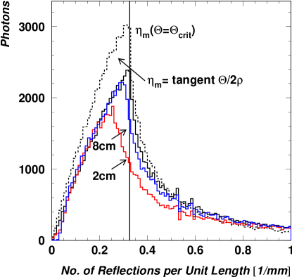
The distribution of the normalised number of reflections, $\eta(\theta)$ , for photons reaching the exit end of straight and curved fibres is shown in figure 6. Again, the figure gives results for curved fibres of two different radii of curvature. The number of reflections a photon experiences scales with the reciprocal of the fibre radius. In the meridional approximation the normalised number of reflections is related by simple trigonometry to the axial angle and the fibre radius: $\eta_{m}(\theta)=\tan{\theta}/2\rho$ . The distribution of $\eta_{m}$ , based on the distribution of axial angles for the trapped photons, is represented by the dashed line. The upper limit, $\eta(\theta_{\it crit})$ , is indicated in the plot by a vertical line. The number of reflections made by a skew ray, $\eta_{s}(\theta)$ , can be calculated for a given skew angle: $\eta_{s}(\theta)=\eta_{m}(\theta)/\cos{\gamma}$ . It is clear that this number increases significantly if the skew angle increases. From the distributions it can be seen that in curved fibres the trapped photons experience fewer reflections on average.

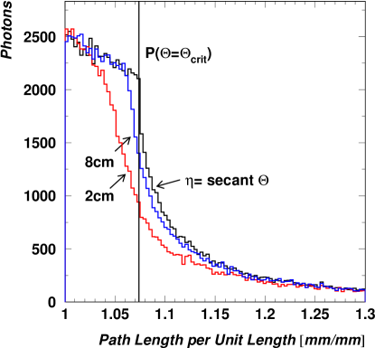
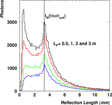
Figure 7(a) shows the distribution of the reflection length, $l_{R}(\theta)$ , for photons reaching the exit end of fibres of radius $\rho=0.6$ mm. The reflection length will scale with the fibre radius. The left figure shows $l_{R}(\theta)$ for four different over-all fibre lengths, $L_{F}=$ 0.5, 1, 2 and 3 m, and the attenuation characteristics of the fibre is made apparent by the non-vanishing attenuation parameters used. Short reflection lengths correspond to long optical path lengths and large numbers of reflections. Because of the many reflections and the long total paths traversed, these photons will be attenuated faster than photons with larger reflection lengths. This reveals the high attenuation of rays with large skew angles. In the meridional approximation the reflection length is related to the axial angle by: $l_{R}=2\rho/\cos{\theta}$ . In the figure the minimum reflection length allowed by the critical angle condition is shown by a vertical line at $l_{R}(\theta_{\it crit})=3.29$ mm. On average photons propagate with smaller reflection lengths along the curved fibre. Figure 7(b) shows the distribution of $l_{R}(\theta)$ in curved fibres of two different radii of curvature, $R_{\it curve}=$ 2 and 8 cm. The fibre radius is identical to the one used in figure (a) and the over-all fibre length is 0.5 m. It can be seen that the sharp peak in the photon distribution flattens with decreasing radius of curvature, so that the region of highest attenuation is close to the reflection length for photons propagating at the critical angle.

In contrast to the analysis of straight fibres an approximation of the sharply curved fibre by meridional rays is not a very good one, since only a very small fraction of the light rays have paths lying in the bending plane. It is clear that when a fibre is curved the path length, the number of reflections and the reflection length of a particular ray in the fibre are affected, which is clearly seen in figures 5, 6 and 7(b). The over-all fibre length for the curved fibres in these calculations is 0.5 m and the fibres are curved for their entire length. The average optical path length and the average number of reflections in a fibre curved over a circular arc are less than those for the same ray in a straight fibre for those photons which remain trapped.

4.3 Light attenuation

Light attenuation in active fibres has many sources, among them self-absorption, optical non-uniformities, reflection losses and absorption by impurities. The two main sources of attenuation in this type of fibres are the absorption of scintillation light and Rayleigh scattering from small density fluctuations. The self-absorption is due to the overlap of the emission and absorption bands of the fluorescent dyes. The cumulative effect of these attenuation processes can be conveniently parameterised by an effective attenuation length over which the signal amplitude is attenuated to 1 $/e$ of its original value, a method often applied in high energy physics applications. The attenuation of active fibres at wavelengths close to its emission band ( $400-600$ nm) is much higher than in wavelength regions of interest for standard applications of communication fibres where mainly infrared light is transmitted ( $0.8-0.9\,\mu$ m and $1.2-1.5\,\mu$ m).

Restricting the analysis to these processes, the transmission through an active fibre can be represented for any given axial angle by $T=\exp\left[-P(\theta)L_{F}/\Lambda_{\it bulk}\right]\,\times q^{\eta(\theta)L_{F}}$ , where the exponential function describes light losses due to bulk absorption and scattering (bulk absorption length $\Lambda_{\it bulk}$ ), and the second factor describes light losses due to imperfect reflections (reflection coefficient $q$ ) which can be caused by a rough surface or variations in the refractive indices. A comparison of some of our own measurements to determine the attenuation length of plastic fibres with other available data indicates that a reasonable value for the bulk absorption length is $\Lambda_{\it bulk}\sim 3$ m. Most published data suggest a deviation of the reflection coefficient, which parameterises the internal reflectivity, from unity between $5\times 10^{-5}$ and $6.5\times 10^{-5}$ [19]. A reasonable value of $q=0.9999$ is used in the simulation to account for all losses proportional to the number of reflections.

Internal reflections being less than total give rise to so-called leaky or non-guided modes, where part of the electromagnetic energy is radiated away. Rays in these modes populate a region defined by axial angles above the critical angle and skew angles slightly larger than the ones for totally internally reflected photons. These modes are taken into account by using the Fresnel equation for the reflection coefficient, $\langle R\rangle$ , averaged over the parallel and orthogonal plane of polarisation

\langle R\rangle=\frac{1}{2}\left(R_{||}+R_{\perp}\right)=\frac{1}{2}\left(\frac{\tan^{2}(\alpha-\beta)}{\tan^{2}(\alpha+\beta)}+\frac{\sin^{2}(\alpha-\beta)}{\sin^{2}(\alpha+\beta)}\right)\ ,

(8)

where $\alpha$ is the angle of incidence and $\beta$ is the refraction angle. However, it is obvious that non-guided modes are lost quickly in a small fibre. This is best seen in the fraction of non-guided to guided modes, $f$ , which decreases from $f=11\%$ at the first reflection of the ray over $f=2.5\%$ at the second reflection to $f<1\%$ at further reflections. Since the average reflection length of non-guided modes is $l_{R}\approx 1.5$ mm those modes do not contribute to the flux transmitted by fibres longer than a few centimeters. The absorption and emission processes in fibres are spread out over a wide band of wavelengths and the attenuation is known to be wavelength dependent. For simplicity only monochromatic light is assumed in the simulation and highly wavelength-dependent effects like Rayleigh scattering are not included explicitly.

A question of practical importance for the estimation of the light output of a particular fibre application is its transmission function. In the meridional approximation and substituting $\exp(-\ln{q})$ by $\exp(1-q)$ the attenuation length can be written as

\Lambda_{m}=\cos{\theta_{\it crit}}\,\left[1/\Lambda_{\it bulk}+(1-q)\sin{\theta_{\it crit}}/2\rho\right]^{-1}\ .

(9)

Only for small diameter fibres ( $D\sim 0.1\,$ mm) are the attenuation lengths due to imperfect reflections of the same order as the absorption lengths. Because of the large radii of the fibres discussed reflection losses are not relevant for the transmission function and the attenuation length contracts to $\Lambda_{m}=\Lambda_{\it bulk}\cos{\theta_{\it crit}}$ . For the simulated bulk absorption length this evaluates to $\Lambda_{m}=2.8$ m. The transmission function outside the meridional approximation can be found by integrating over the normalised path length distribution, where $dN$ represents the number of photons per path length interval $dP$ , weighted by the exponential bulk absorption factor:

T=\frac{1}{N}\int_{P=0}^{\infty}dN/dP\,e^{-PL_{F}/\Lambda_{\it bulk}}\,dP\ .

(10)

Figure 8 shows this transmission function versus the ratio of fibre to absorption length, $L_{F}/\Lambda_{m}$ . A simple exponential fit, $T\propto\exp\left[-L_{F}/\Lambda_{\it eff}\right]$ , applied to the simulated light transmissions for a varying fibre length results in an effective attenuation length of $\Lambda_{\it eff}=2.4$ m. For $L_{F}/\Lambda_{m}\geq 0.2$ this description is sufficiently accurate to parameterise the transmission function, at smaller values for $L_{F}/\Lambda_{m}$ the light is attenuated faster. The difference of order 15% to the meridional attenuation length is attributed to the tail of the path length distribution.

Measurements of the light attenuation in fibres proves this simple model of a single attenuation length to be wrong. A dependence of the attenuation length with distance usually is observed [20]. The most important cause of this effect is the fact that the short wavelength components of the scintillation light is dominantly absorbed. This leads to a shift of the average wavelength in the emission spectrum towards longer wavelengths and to an increase in the effective attenuation length.

4.4 Trapping efficiency and transition losses in sharply curved fibres

One of the most important practical issues in implementing optical fibres into compact particle detector systems are macro-bending losses. In general, some design parameters of fibre applications, especially if the over-all size of the detector system is important, depend crucially on the minimum permissible radius of curvature. By using waveguide analysis transition and bending losses have been thoroughly investigated and a loss formula in terms of the Poynting vector can be derived [21, 22]. Those studies are difficult to extend to multimode fibres since a large number of guided modes has to be considered. When applying ray optics to curved multimode fibres the use of a two-dimensional model is common [11, 12, 13]. In contrast, our simulation method follows a three-dimensional approach.

Photons are lost from a fibre core both by refraction and tunnelling. In the simulation only refracting photons were considered. The angle of incidence of a light ray at the tensile (outer) side of the fibre is always smaller than at the compressed side and photons propagate either by reflections on both sides or in the extreme meridional case by reflections on the tensile side only. If the fibre is curved over an arc of constant radius of curvature photons can be refracted, and will then no longer be trapped, at the very first reflection point on tensile side. Therefore, the trapping efficiency for photons entering a curved section of fibre towards the tensile side is reduced most. Figure 9 quantifies the dependence of the trapping efficiency on the azimuthal angle, $\Psi$ , between the bending plane and the photon path for a curved fibre with a radius of curvature $R_{\it curve}=$ 2 cm. The azimuthal angle is orthogonal to the axial angle and $\Psi=0\,$ rad corresponds to photons emitted towards the tensile side of the fibre.

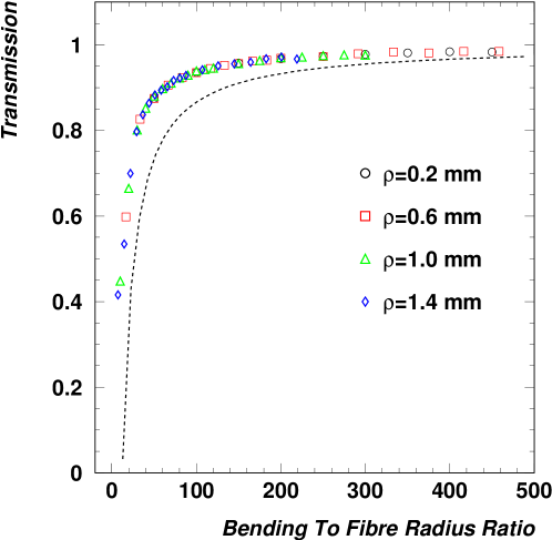
Figure 10 displays the explicit dependence of the transmission function for fibres curved over circular arcs of 90^∘ on the radius of curvature to fibre radius ratio for different fibre radii, $\rho=$ 0.2, 0.6, 1.0 and 1.2 mm. No further light attenuation is assumed. Evidently, the number of photons which are refracted out of a sharply curved fibre increases very rapidly with decreasing radius of curvature. The losses are dependent only on the curvature to fibre radius ratio, since no inherent length scale is involved, justifying the introduction of this scaling variable. The light loss due to bending of the fibre is about 10% for a radius of curvature of 65 times the fibre radius.

The use of the meridional approximation in the bending plane in place of a three dimensional fibre is justified by the losses being dominantly caused by meridional rays [23, 10]. Figure 11 shows a section of a curved fibre and the passage of a meridional ray in the bending plane with maximum axial angle. In this model photons are guided for axial angles

\cos\theta<\cos\theta_{O}=\frac{R+2\rho}{R+\rho}\cos\theta_{\it crit}\ ,

(11)

where the subscript $O$ refers to the outer fibre wall. A transmission function can be estimated by assuming that all photons with axial angles $\theta>\theta_{O}$ are refracted out of the fibre:

T=1-\frac{1}{1+R_{\it curve}/\rho}\ \frac{\cos\theta_{\it crit}}{1-\cos\theta_{\it crit}}\ .

(12)

This transmission function is shown in figure 10 as a dashed line and it overestimates the light losses due the larger axial angles allowed for skew rays. A comparable theoretical calculation using a two-dimensional slab model and a generalized Fresnel transmission coefficient has been performed by Badar et al [12]. Their plot of the power contained in the fibre core as a function of the radius of curvature (figure 5) is similar to our results on the transmission function in the meridional approximation. In [10] a ray optics calculation for curved multimode fibres involving skew rays is presented. In this paper a discussion on the transmission function is missing. Instead, a plot of the power remaining in a curved fibre versus distance is shown which gives complementary information.

For photons entering a curved section of fibre the first point of reflection on the tensile side defines the transition angle, $\Phi_{\it trans}$ , measured from the plane of entry. The angular range of transition angles associated with each ray is called the transition region of the fibre. For photons emitted towards the tensile side the transition angle is related to the axial angle and since the angular phase space density of trapped photons is highest close to the critical angle a good estimate is $\Phi_{\it trans}=\theta_{\it crit}-\theta_{O}$ . For a fibre radius $\rho=$ 0.6 mm and radii of curvature $R_{\it curve}=$ 1, 2, and 5 cm the above formula leads to transition angles $\Phi_{\it trans}=$ 0.19, 0.08 and 0.03 rad, respectively. We attribute these discrete angles to beams emitted in the bending plane. Photons emitted from the fibre axis towards the compressed side are not lost at this side, however, they experience at least one reflection on the tensile side if the bending angle exceeds the limit $\Phi_{\it limit}=\arccos\left[R_{\it curve}/(R_{\it curve}+2\,\rho)\right]\approx\arccos\left[1-2\,\rho/R_{\it curve}\right]$ . A transition in the transmission function should occur at bending angles between $\Phi_{\it limit}/2$ , where all photons emitted towards the tensile side have experienced a reflection, and $\Phi_{\it limit}$ , where this is true for all photons. Figure 12 shows the transmission as a function of bending angle, $\Phi$ , for a standard fibre as defined before. Once a sharply curved fibre with a ratio $R_{\it curve}/\rho>83$ is bent through angles $\Phi\sim\pi/8$ rad light losses do not increase any further. The transition region ranges from $\sim 0.44$ to $\sim 1.06$ rad and is indicated in the figure by arrows. At much smaller ratios $R_{\it curve}/\rho$ the model is no longer valid to describe this behaviour.

Experimental results on losses in curved multimode fibres along with corresponding predictions are best known for silica fibres with core radii $\rho\approx 50\,\mu$ m. Calculations on the basis of ray optics for a plastic fibre with $\rho=0.49\,$ mm can be found in [13]. Our result on the transmission function in the meridional approximation $T=0.35$ at $\rho/R_{\it curve}=$ 20 is in good agreement with the two-dimensional calculation. The larger value of $T=0.65$ predicted by the simulation is explained by the small loss of skew rays, clearly seen in figure 7. It should be noted that the difference between finite and infinite cladding and the appearance of oscillatory losses in the transition region has not been investigated in the simulation.

Figure 3 shows contours of the angular phase space for photons which were trapped in the straight fibre section but are refracted out of sharply curved fibres with radii of curvature $R_{\it curve}=$ 2 and 5 cm. The contours demonstrate that only skew rays from a small region close to the boundary curve are getting lost. The smaller the radius of curvature, the larger the affected phase space region.

4.5 Light dispersion

The timing resolution of scintillators are often of paramount importance, but a pulse of light, consisting of several photons propagating along a fibre, broadens in time. In active fibres, three effects are responsible for the time distribution of photons reaching the fibre exit end. Firstly the decay time of the fluorescent dopants, usually of the order of a few nanoseconds, secondly the chromatic dispersion in a dispersive medium, and thirdly the fact that photons on different paths have different transit times to reach the fibre exit end, known as inter-modal dispersion.

The chromatic dispersion is due to the spectral width, $\Delta\lambda$ , of the emitter. It is the combination of material dispersion and waveguide dispersion. If the core refractive index is explicitly dependent on the wavelength, $n(\lambda)$ , photons of different wavelengths have different propagation velocities along the same path, called material dispersion. The broadening of a pulse is given by $\Delta\tau=L_{F}/c_{\it core}\left(\lambda^{2}d^{2}n/d\lambda^{2}\right)\Delta\lambda/\lambda$ [9]. The FWHM of the emission peaks of scintillating or wavelength-shifting fibres is approximately $40-50$ nm. The material dispersion in the used polymers (mostly polystyrene) is of the order of ns $/$ nm $\times$ km and thus negligible for multimode fibres.

The transit time in ray optics is simply given by $\tau=P(\theta)/c_{\it core}$ , where $c_{\it core}$ is the speed of light in the fibre core. The simulation results on the transit time are shown in figure 13. The full widths at half maximum (FWHM) of the pulses in the time spectrum are presented for four different fibre lengths. The resulting dispersion has to be compared with the time dispersion in the meridional approximation which is simply the difference between the shortest transit time $\tau(\theta=0)$ and the longest transit time $\tau(\theta=\theta_{\it crit})$ : $\Delta\tau=L_{F}/c_{\it core}\ (\sec{\theta_{\it crit}}-1)$ , where $L_{F}$ is the total axial length of the fibre. The dispersion evaluates for the different fibre lengths to 197 ps for 0.5 m, 393 ps for 1 m, 787 ps for 2 m and 1181 ps for 3 m. Those numbers are in good agreement with the simulation, although there are tails associated to the propagation of skew rays. With the attenuation parameters of our simulation the fraction of photons arriving later than $\tau(\theta=\theta_{\it crit})$ decreases from 37.9% for a 0.5 m fibre to 32% for a 3 m fibre due to the stronger attenuation of the skew rays in the tail. Due to inter-modal dispersion the pulse broadening is quite significant.

5 Summary

We have simulated the propagation of photons in straight and curved optical fibres. The simulations have been used to evaluate the loss of photons propagating in fibres curved in a circular path in one plane. The results show that loss of photons due to the curvature of the fibre is a simple function of radius of curvature to fibre radius ratio and is $<10\%$ if the ratio is $>65$ . The simulations also show that for larger ratios this loss takes place in a transition region ( $\Phi\sim\pi/8$ ) during which a new distribution of photon angles is established. Photons which survive the transition region then propagate without further losses.

We have also used the simulation to investigate the dispersion of transit times of photons propagating in straight fibres. For fibre lengths between 0.5 and 3 m we find that approximately two thirds of the photons arrive within the spread of transit times which would be expected from the use of the simple meridional ray approximation and the refractive index of the fibre core. The remainder of the photons arrive in a tail at later times due to their helical paths in the fibre. The fraction of photons in the tail of the distribution decreases only slowly with increasing fibre length and will depend on the attenuation parameters of the fibre.

We find that when realistic bulk absorption and reflection losses are included in the simulation for a straight fibre, the overall transmission can not be described by a simple exponential function of propagation distance because of the large spread in optical path lengths between the most meridional and most skew rays.

We anticipate that these results on the magnitude of transition losses will be of use for the design of particle detectors incorporating sharply curved active fibres.

This research was supported by the UK Particle Physics and Astronomy Research Council (PPARC).

References

[1] Leutz H 1995 Scintillating fibres Nucl. Instrum. Methods Phys. Res. A 364 422–48
[2] ATLAS Collaboration 1994 Technical proposal for a general purpose $pp$ experiment at the LHC at CERN, CERN/LHCC/94-43
[3] MINOS Collaboration 1998 The MINOS Detectors, Technical Design Report, Fermilab, NuMI-L-337
[4] Snitzer E 1961 Cylindrical dielectric waveguide modes J. Opt. Soc. Am. 51 491–8
[5] Kapany N S, Burke J J and Shaw C C 1963 Fiber optics. X. Evanescent boundary wave propagation J. Opt. Soc. Am. 53 929–35
[6] Kapany N S 1957 Fiber optics. I. Optical properties of certain dielectric cylinders J. Opt. Soc. Am. 47 413–22
[7] Kapany N S 1967 Fibre Optics: Principles and Applications (New York: Academic)
[8] Allan W B 1973 Fibre Optics: Theory and Practice, Optical Physics and Engineering (London: Plenum)
[9] Ghatak A and Thyagarajan K 1998 Introduction to Fiber Optics (Cambridge: Cambridge University Press)
[10] Winkler C, Love J D and Ghatak A K 1979 Loss calculation in bent multimode optical waveguides Opt. Quantum Electron. 11 173–83.
[11] Badar A H, Maclean T S M, Gazey B K, Miller J F and Ghafoori-Shiraz H 1989 Radiation from circular bends in multimode and single-mode optical fibres IEE Proc. J 136 147–51
[12] Badar A H, Maclean T S M, Ghafoori-Shiraz H and Gazey B K 1991 Bent slab ray theory for power distribution in core and cladding of bent multimode optical fibres IEE Proc. J 138 7–12
[13] Badar A H and Maclean T S M 1991 Transition and pure bending losses in multimode and single-mode bent optical fibres IEE Proc. J 138 261–8
[14] Potter R J 1961 Transmission properties of optical fibers J. Opt. Soc. Am. 51 1079–89
[15] Kapany N S and Capellaro D F 1961 Fiber optics. VII. Image transfer from Lambertian emitters J. Opt. Soc. Am. 51 23–31 (appendix: Geometrical optics of straight circular dielectric cylinder)
[16] Potter R J, Donath E and Tynan R 1963 Light-collecting properties of a perfect circular optical fiber J. Opt. Soc. Am. 53 256–60
[17] Press W H, Teukolsky S A, Vetterling W T and Flannery B P 1992 Numerical recipes in Fortran77: the art of scientific computing Fortran Numerical Recipes vol 1, 2nd edn (Cambridge: Cambridge University Press)
[18] Johnson K F 1994 Achieving the theoretical maximum light yield in scintillating fibres through non-uniform doping Nucl. Instrum. Methods Phys. Res. A 344 432–34
[19] D’Ambrosio C, Leutz H and Taufer M 1991 Reflection losses in polysterene fibres Nucl. Instrum. Methods Phys. Res. A 306 549–56
[20] Davis A J, Hink P, Binns W, Epstein J, Connell J, Israel M, Klarmann J, Vylet V, Kaplan D and Reucroft S 1989 Scintillating optical fiber trajectory detectors Nucl. Instrum. Methods Phys. Res. A 276 347–58
[21] Marcuse D 1976 Curvature loss formula for optical fibers J. Opt. Soc. Am. 66 216–20
[22] Gambling W A, Matsumura H and Ragdale C M 1979 Curvature and microbending losses in single-mode optical fibres Opt. Quantum Electron. 11 43–59
[23] Gloge D 1972 Bending loss in multimode fibers with graded and ungraded core index Appl. Opt. 11 2506–13

Refer to caption — Figure 1: (a) Definition of the angles for a skew ray from an initial point, $\vec{r}$ to a point of reflection, $\vec{r}_{R}$ , on the core-cladding interface. The axial angle of the ray is $\theta$ . The angle between the projection of the ray in a plane perpendicular to the axis of the fibre with respect to the normal at the point of reflection, $\gamma$ , defines the ray’s ‘skewness’. The angle of incidence at the point of reflection is $\alpha$ . (b) The helical path of a skew ray in a fibre of radius $\rho=0.6\,$ mm which spirals along the core-cladding interface. The $z$ -axis represents the axial fibre length and the fibre cross-section lies in the $xy$ -plane.

Figure 2: A scheme on the main steps of the program to generate and track photons in fibres of constant curvature. The equations to find the intersection of the light ray with the core-cladding interface are solved by numerical methods.