How to Measure Specific Heat
Using Event-by-Event Average pTsubscript𝑝𝑇p_{T} Fluctuations.

M.Β J.Β Tannenbaum Research supported by U.S. Department of Energy, DE-AC02-98CH10886. Brookhaven National Laboratory
Upton, NY 11973-5000 USA
for the PHENIX Collaboration
Email: mjt@bnl.gov
Abstract

A simple way to visualize event-by-event average pTsubscript𝑝𝑇p_{T} fluctuations is by assuming that each collision has a different temperature parameter (inverse pTsubscript𝑝𝑇p_{T} slope) and that the ensemble of events has a temperature distribution about the mean, ⟨T⟩delimited-βŸ¨βŸ©π‘‡\langle T\rangle, with standard deviation ΟƒTsubscriptπœŽπ‘‡\sigma_{T}. PHENIX characterizes the non-random fluctuation of MpTsubscript𝑀subscript𝑝𝑇M_{p_{T}}, the event-by-event average pTsubscript𝑝𝑇p_{T}, by FpTsubscript𝐹subscript𝑝𝑇F_{p_{T}}, the fractional difference of the standard deviation of the data from that of a random sample obtained with mixed events. This can be related to the temperature fluctuation:

FpT=ΟƒMpTdata/ΟƒMpTrandomβˆ’1≃(⟨nβŸ©βˆ’1)​σT2/⟨T⟩2.subscript𝐹subscript𝑝𝑇subscriptsuperscript𝜎datasubscript𝑀subscript𝑝𝑇subscriptsuperscript𝜎randomsubscript𝑀subscript𝑝𝑇1similar-to-or-equalsdelimited-βŸ¨βŸ©π‘›1subscriptsuperscript𝜎2𝑇superscriptdelimited-βŸ¨βŸ©π‘‡2F_{p_{T}}=\sigma^{\rm data}_{M_{p_{T}}}/\sigma^{\rm random}_{M_{p_{T}}}-1\simeq(\langle n\rangle-1)\sigma^{2}_{T}/\langle T\rangle^{2}\qquad.

Combining this with the Gavai, et al.,Gavai05 and Korus, et al.,Korus definitions of the specific heat per particle, a simple relationship is obtained:

cv/T3=⟨n⟩⟨Nt​o​tβŸ©β€‹1FpT.subscript𝑐𝑣superscript𝑇3delimited-βŸ¨βŸ©π‘›delimited-⟨⟩subscriptπ‘π‘‘π‘œπ‘‘1subscript𝐹subscript𝑝𝑇c_{v}/T^{3}={\left<n\right>\over\left<N_{tot}\right>}{1\over F_{p_{T}}}\qquad.

FpTsubscript𝐹subscript𝑝𝑇F_{p_{T}} is measured with a fraction ⟨n⟩/⟨Nt​o​t⟩delimited-βŸ¨βŸ©π‘›delimited-⟨⟩subscriptπ‘π‘‘π‘œπ‘‘\left<n\right>/\left<N_{tot}\right> of the total particles produced, a purely geometrical factor representing the fractional acceptance, ∼1/33similar-toabsent133\sim 1/33 in PHENIX. Gavai, et al. predict that cv/T3=15subscript𝑐𝑣superscript𝑇315c_{v}/T^{3}=15, which corresponds to FpT∼0.20similar-tosubscript𝐹subscript𝑝𝑇0.20F_{p_{T}}\sim 0.20% in PHENIX, which may be accessible by measurements of MpTsubscript𝑀subscript𝑝𝑇M_{p_{T}} in the range 0.2≀pT≀0.60.2subscript𝑝𝑇0.60.2\leq p_{T}\leq 0.6 GeV/c. In order to test the Gavai, et al. prediction that cv/T3subscript𝑐𝑣superscript𝑇3c_{v}/T^{3} is reduced in a QGP compared to the ideal gas value (15 compared to 21), precision measurements of FpTsubscript𝐹subscript𝑝𝑇F_{p_{T}} in the range 0.20% for 0.2≀pT≀0.60.2subscript𝑝𝑇0.60.2\leq p_{T}\leq 0.6 GeV/c may be practical.

pacs:
24.60.-k, 25.75.-q, 25.75.Gz

I Introduction

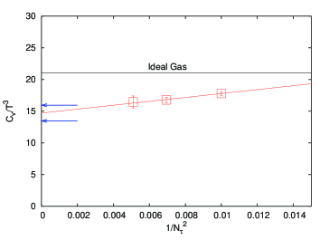
R. Gavai, S. Gupta and S. MukherjeeΒ Gavai05 predict in β€œquenched QCD” at 2​Tc2subscript𝑇𝑐2T_{c} and 3​Tc3subscript𝑇𝑐3T_{c} that the specific heat, cV/T3subscript𝑐𝑉superscript𝑇3c_{V}/T^{3}, differs significantly from the value for an ideal gasβ€”15 compared to 21 (see Fig.Β 1). Can this be measured?

Refer to caption
Figure 1: Gavai, et al., prediction for cv/T3subscript𝑐𝑣superscript𝑇3c_{v}/T^{3}Β Gavai05 .

II Event-by-event average pTsubscript𝑝𝑇p_{T} fluctuations and Specific Heat

II.1 Single particle distributions

The single particle transverse momentum (pTsubscript𝑝𝑇p_{T}) distribution averaged over all particles in all events for a p-p experiment (inclusive) or in all events of a given centrality class for an A+A experiment (semi-inclusive) is usually written in the form:

d​σd​pT=bΓ​(p)​(b​pT)pβˆ’1​eβˆ’b​pTord​σpT​d​pT=b2Γ​(p)​(b​pT)pβˆ’2​eβˆ’b​pT.formulae-sequenceπ‘‘πœŽπ‘‘subscript𝑝𝑇𝑏Γ𝑝superscript𝑏subscript𝑝𝑇𝑝1superscript𝑒𝑏subscript𝑝𝑇orπ‘‘πœŽsubscript𝑝𝑇𝑑subscript𝑝𝑇superscript𝑏2Γ𝑝superscript𝑏subscript𝑝𝑇𝑝2superscript𝑒𝑏subscript𝑝𝑇{d\sigma\over{dp_{T}}}={b\over{\Gamma(p)}}{(bp_{T})}^{p-1}e^{-bp_{T}}\qquad\mbox{or}\qquad{d\sigma\over{p_{T}dp_{T}}}={{b^{2}}\over{\Gamma(p)}}{(bp_{T})}^{p-2}e^{-bp_{T}}\qquad. (1)

EquationΒ 1 represents a Gamma distribution, where ⟨pT⟩=p/bdelimited-⟨⟩subscript𝑝𝑇𝑝𝑏\langle p_{T}\rangle=p/b, ΟƒpT/⟨pT⟩=1/psubscript𝜎subscript𝑝𝑇delimited-⟨⟩subscript𝑝𝑇1𝑝\sigma_{p_{T}}/\langle p_{T}\rangle=1/\sqrt{p}. Typically b=6𝑏6b=6 (GeV/c)-1 and p=2𝑝2p=2 for p-p collisions. As shown in Fig.Β 2, the p𝑝p parameter depends on the particle type in central Au+Au collisions, with p<2𝑝2p<2 for π±superscriptπœ‹plus-or-minus\pi^{\pm}, p∼2similar-to𝑝2p\sim 2 for KΒ±superscript𝐾plus-or-minusK^{\pm} and p>2𝑝2p>2 for (anti-) protons, but the asymptotic slope tends to be the same for all particles. The β€˜inverse slope parameter’, T=1/b𝑇1𝑏T=1/b, is usually referred to as the β€˜Temperature parameter’.

Refer to caption
Figure 2: Identified particle semi-inclusive invariant pTsubscript𝑝𝑇p_{T} spectra for Au+Au central collisionsΒ PX026 . At the lowest pTsubscript𝑝𝑇p_{T}, the Ο€+superscriptπœ‹\pi^{+} are the highest, followed by K+superscript𝐾K^{+} and p𝑝p (left) and the same for the negatives (right).

II.2 Event-by-Event Average

For events with n𝑛n detected charged particles with magnitudes of transverse momenta, pTisubscript𝑝subscript𝑇𝑖p_{T_{i}}, the event-by-event average pTsubscript𝑝𝑇p_{T}, denoted MpTsubscript𝑀subscript𝑝𝑇M_{p_{T}}, is defined as:

MpT=pTΒ―=1nβ€‹βˆ‘i=1npTi.subscript𝑀subscript𝑝𝑇¯subscript𝑝𝑇1𝑛superscriptsubscript𝑖1𝑛subscript𝑝subscript𝑇𝑖M_{p_{T}}=\overline{p_{T}}={1\over n}\sum_{i=1}^{n}p_{T_{i}}\qquad. (2)

By definition ⟨MpTβŸ©β‰‘βŸ¨pT⟩=ΞΌdelimited-⟨⟩subscript𝑀subscript𝑝𝑇delimited-⟨⟩subscriptπ‘π‘‡πœ‡\left<M_{p_{T}}\right>\equiv\left<p_{T}\right>=\mu; however, it takes hard work to make one’s data follow this identity to high precision (β‰ͺ1%much-less-thanabsentpercent1\ll 1\%). The standard deviation of MpTsubscript𝑀subscript𝑝𝑇M_{p_{T}} is defined the usual way:

ΟƒMpT2β‰‘βŸ¨MpT2βŸ©βˆ’βŸ¨MpT⟩2=1n2​(n​σpT2+βˆ‘i=1nβˆ‘j=1,jβ‰ in⟨(pTiβˆ’βŸ¨pT⟩)​(pTjβˆ’βŸ¨pT⟩)⟩).subscriptsuperscript𝜎2subscript𝑀subscript𝑝𝑇delimited-⟨⟩subscriptsuperscript𝑀2subscript𝑝𝑇superscriptdelimited-⟨⟩subscript𝑀subscript𝑝𝑇21superscript𝑛2𝑛subscriptsuperscript𝜎2subscript𝑝𝑇superscriptsubscript𝑖1𝑛superscriptsubscriptformulae-sequence𝑗1𝑗𝑖𝑛delimited-⟨⟩subscript𝑝subscript𝑇𝑖delimited-⟨⟩subscript𝑝𝑇subscript𝑝subscript𝑇𝑗delimited-⟨⟩subscript𝑝𝑇\sigma^{2}_{M_{p_{T}}}\equiv\left<M^{2}_{p_{T}}\right>-\left<M_{p_{T}}\right>^{2}={1\over n^{2}}\left(n\sigma^{2}_{p_{T}}+\sum_{i=1}^{n}\sum_{j=1,j\neq i}^{n}\left\langle{(p_{T_{i}}-\langle p_{T}\rangle)(p_{T_{j}}-\langle p_{T}\rangle)}\right\rangle\right)\qquad. (3)

If all the pTisubscript𝑝subscript𝑇𝑖p_{T_{i}} on all events are random samples of the same pTsubscript𝑝𝑇p_{T} distribution, then:

ΟƒMpT2=ΟƒpT2n,subscriptsuperscript𝜎2subscript𝑀subscript𝑝𝑇subscriptsuperscript𝜎2subscript𝑝𝑇𝑛\sigma^{2}_{M_{p_{T}}}={\sigma^{2}_{p_{T}}\over n}\qquad, (4)

where ΟƒpT=⟨pT2βŸ©βˆ’βŸ¨pT⟩2subscript𝜎subscript𝑝𝑇delimited-⟨⟩superscriptsubscript𝑝𝑇2superscriptdelimited-⟨⟩subscript𝑝𝑇2\sigma_{p_{T}}=\sqrt{\left<p_{T}^{2}\right>-\left<p_{T}\right>^{2}} is the standard deviation of Eq.Β 1, the inclusive pTsubscript𝑝𝑇p_{T} spectrum (averaged over all events).

A nice illustration of what can be revealed by the event-by-event average that is not shown by the inclusive average over all events was given by Korus, et al.Β Korus . Suppose that each collision has a different temperature parameter such that the ensemble of events has a mean, ⟨T⟩delimited-βŸ¨βŸ©π‘‡\left<T\right>, with standard deviation, ΟƒT=⟨T2βŸ©βˆ’βŸ¨T⟩2subscriptπœŽπ‘‡delimited-⟨⟩superscript𝑇2superscriptdelimited-βŸ¨βŸ©π‘‡2\sigma_{T}=\sqrt{\left<T^{2}\right>-\left<T\right>^{2}}, about the mean. It is easy to show that for this case:

ΟƒMpT2ΞΌ2βˆ’1n​σpT2ΞΌ2=(1βˆ’1n)​σT2⟨T⟩2.subscriptsuperscript𝜎2subscript𝑀subscript𝑝𝑇superscriptπœ‡21𝑛subscriptsuperscript𝜎2subscript𝑝𝑇superscriptπœ‡211𝑛subscriptsuperscript𝜎2𝑇superscriptdelimited-βŸ¨βŸ©π‘‡2{{\sigma^{2}_{M_{p_{T}}}}\over\mu^{2}}-{1\over n}{\sigma^{2}_{p_{T}}\over\mu^{2}}=(1-{1\over n}){\sigma^{2}_{T}\over\left<T\right>^{2}}\qquad. (5)

II.3 Specific Heat

As pointed out by Korus, et al.,Korus if the parameter T𝑇T would correspond to the actual temperature of the system, not just the inverse slope of the pTsubscript𝑝𝑇p_{T} distribution, then a basic equation of thermodynamics would relate the temperature fluctuations of a system to its total heat capacityΒ Stodolsky ; Shuryak ; Rajagopal :

1CV=ΟƒT2⟨T⟩2,1subscript𝐢𝑉subscriptsuperscript𝜎2𝑇superscriptdelimited-βŸ¨βŸ©π‘‡2{1\over C_{V}}={{\sigma^{2}_{T}}\over{\left<T\right>^{2}}}\qquad, (6)

where CVsubscript𝐢𝑉C_{V} is an extensive quantity corresponding to the total number of particles in the system, ⟨Nt​o​t⟩delimited-⟨⟩subscriptπ‘π‘‘π‘œπ‘‘\left<N_{tot}\right>. Thus the specific heat per particle is cV=CV/⟨Nt​o​t⟩subscript𝑐𝑉subscript𝐢𝑉delimited-⟨⟩subscriptπ‘π‘‘π‘œπ‘‘c_{V}=C_{V}/\left<N_{tot}\right>. Gavai, et al.,Gavai05 refer to this same (dimensionless) quantity as cv/T3subscript𝑐𝑣superscript𝑇3c_{v}/T^{3}, resulting in the final equation:

cvT3=1⟨Nt​o​tβŸ©β€‹1ΟƒT2/⟨T⟩2subscript𝑐𝑣superscript𝑇31delimited-⟨⟩subscriptπ‘π‘‘π‘œπ‘‘1subscriptsuperscript𝜎2𝑇superscriptdelimited-βŸ¨βŸ©π‘‡2{c_{v}\over T^{3}}={1\over{\langle N_{tot}\rangle}}\frac{1}{\sigma^{2}_{T}/\langle T\rangle^{2}} (7)

where n𝑛n represents the number of particles used in the calculation of MpTsubscript𝑀subscript𝑝𝑇M_{p_{T}} (Eq.Β 5) from which ΟƒT/⟨T⟩subscriptπœŽπ‘‡delimited-βŸ¨βŸ©π‘‡\sigma_{T}/\left<T\right> is determined.

III Measurements of MpTsubscript𝑀subscript𝑝𝑇M_{p_{T}}

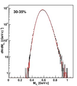
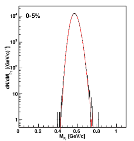
The measured MpTsubscript𝑀subscript𝑝𝑇M_{p_{T}} distributions for two centrality classes in sN​N=200subscript𝑠𝑁𝑁200\sqrt{s_{NN}}=200 GeV Au+Au collisions in PHENIXΒ PX200 are shown in FigureΒ 3 (data points) compared to a random baseline (histograms). Mixed-events are used to define the baseline for random fluctuations of MpTsubscript𝑀subscript𝑝𝑇M_{p_{T}}. This has the advantage of effectively removing any residual detector-dependent effects. The event-by-event average distributions are very sensitive to the number of tracks in the event (denoted n𝑛n), so the mixed event sample is produced with the identical n𝑛n distribution as the data. Additionally, no two tracks from the same data event are placed in the same mixed event in order to remove any intra-event correlations in pTsubscript𝑝𝑇p_{T}. Finally, ⟨MpT⟩delimited-⟨⟩subscript𝑀subscript𝑝𝑇\langle M_{p_{T}}\rangle must exactly match the semi-inclusive ⟨pT⟩delimited-⟨⟩subscript𝑝𝑇\langle p_{T}\rangle.

Refer to caption Refer to caption
Figure 3: MpTsubscript𝑀subscript𝑝𝑇M_{p_{T}} for 30-35% and 0-5% centrality classesPX200 : data (points) mixed-events (histogram).

The non-Gaussian, Gamma distribution shape of the MpTsubscript𝑀subscript𝑝𝑇M_{p_{T}} distributions is evident. The difference between the data and the mixed-event random baseline distributions is barely visible to the naked eye. PHENIX quantifies the non-random fluctuation by the fractional difference of the standard deviations of MpTsubscript𝑀subscript𝑝𝑇M_{p_{T}} for the data and the mixed-event (random) sample:

FpT≑σMpT,dataβˆ’ΟƒMpT,mixedΟƒMpT,mixed,subscript𝐹subscript𝑝𝑇subscript𝜎subscript𝑀subscript𝑝𝑇datasubscript𝜎subscript𝑀subscript𝑝𝑇mixedsubscript𝜎subscript𝑀subscript𝑝𝑇mixedF_{p_{T}}\equiv\frac{\sigma_{M_{p_{T}},{\rm data}}-\sigma_{M_{p_{T}},{\rm mixed}}}{\sigma_{M_{p_{T}},{\rm mixed}}}\qquad, (8)

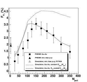
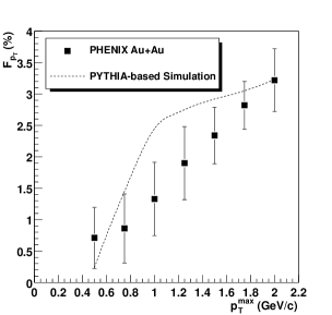
which is on the order of a few percent. The results are shown (Fig.Β 4-left) as a function of centrality (represented by Np​a​r​tsubscriptπ‘π‘π‘Žπ‘Ÿπ‘‘N_{part}) for charged particle tracks in the range 0.2 GeV/c ≀pT≀2.0absentsubscript𝑝𝑇2.0\leq p_{T}\leq 2.0 GeV/c; and, for the 20-25% centrality class (Np​a​r​t=181.6subscriptπ‘π‘π‘Žπ‘Ÿπ‘‘181.6N_{part}=181.6), over a varying pTsubscript𝑝𝑇p_{T} range, 0.2 GeV/c ≀pT≀pTmaxabsentsubscript𝑝𝑇superscriptsubscript𝑝𝑇max\leq p_{T}\leq p_{T}^{\rm max} (FigureΒ 4-right).

Refer to caption Refer to caption
Figure 4: FpTsubscript𝐹subscript𝑝𝑇F_{p_{T}} vs centrality and pTmaxsuperscriptsubscript𝑝𝑇maxp_{T}^{\rm max} compared to simulationsΒ PX200 .

The steep increase in FpTsubscript𝐹subscript𝑝𝑇F_{p_{T}} for the small increase in the number of tracks with increasing pTmax>1superscriptsubscript𝑝𝑇max1p_{T}^{\rm max}>1 GeV/c is consistent with correlations due to jet production as shown by the dotted linesΒ PX200 . However, other explanations have been proposedΒ Ferreiro . Note that the errors are entirely systematic, due to time-dependent detector variations. Comparatively, statistical errors are negligible.

IV How to measure cv/T3subscript𝑐𝑣superscript𝑇3c_{v}/T^{3}.

For the small values of FpTsubscript𝐹subscript𝑝𝑇F_{p_{T}} observed, one can make use of the identity

Δ​σ2Οƒ2=2​Δ​σσ=2​FΞ”superscript𝜎2superscript𝜎22Ξ”πœŽπœŽ2𝐹{{\Delta\sigma^{2}}\over{\sigma^{2}}}=2{{\Delta\sigma}\over{\sigma}}=2F (9)

to obtain the relation:

(1βˆ’1n)​σT2T2=ΟƒMpT2ΞΌ2βˆ’1n​σpT2ΞΌ2=2​FpT​1n​σpT2ΞΌ2=2​FpTn​p≃FpTn.11𝑛subscriptsuperscript𝜎2𝑇superscript𝑇2subscriptsuperscript𝜎2subscript𝑀subscript𝑝𝑇superscriptπœ‡21𝑛subscriptsuperscript𝜎2subscript𝑝𝑇superscriptπœ‡22subscript𝐹subscript𝑝𝑇1𝑛subscriptsuperscript𝜎2subscript𝑝𝑇superscriptπœ‡22subscript𝐹subscript𝑝𝑇𝑛𝑝similar-to-or-equalssubscript𝐹subscript𝑝𝑇𝑛(1-{1\over n}){\sigma^{2}_{T}\over T^{2}}={{\sigma^{2}_{M_{p_{T}}}}\over\mu^{2}}-{1\over n}{\sigma^{2}_{p_{T}}\over\mu^{2}}=2F_{p_{T}}{1\over n}{{\sigma^{2}_{p_{T}}}\over\mu^{2}}={{2F_{p_{T}}}\over{np}}\simeq{F_{p_{T}}\over n}\qquad. (10)

Combining Eq.Β 10 with Eq.Β 7, we obtain the simple and elegant expression:

cvT3=⟨n⟩⟨Nt​o​tβŸ©β€‹1FpT.subscript𝑐𝑣superscript𝑇3delimited-βŸ¨βŸ©π‘›delimited-⟨⟩subscriptπ‘π‘‘π‘œπ‘‘1subscript𝐹subscript𝑝𝑇{c_{v}\over T^{3}}={{\langle n\rangle}\over{\langle N_{tot}\rangle}}\frac{1}{F_{p_{T}}}\qquad. (11)

Note that FpTsubscript𝐹subscript𝑝𝑇F_{p_{T}} is measured with a fraction ⟨n⟩/⟨Nt​o​t⟩delimited-βŸ¨βŸ©π‘›delimited-⟨⟩subscriptπ‘π‘‘π‘œπ‘‘\left<n\right>/\left<N_{tot}\right> of the total particles produced, which is a purely geometrical factor representing the fractional acceptance of the measurement. For example, if all particles are produced in a range δ​ηFWHM𝛿subscriptπœ‚FWHM\delta\eta_{\rm FWHM} (assuming a flat or trapezoidal d​n/dβ€‹Ξ·π‘‘π‘›π‘‘πœ‚dn/d\eta over this interval) and if including the neutrals gives a factor of 1.5 more total particles than charged particles; and if FpTsubscript𝐹subscript𝑝𝑇F_{p_{T}} is measured with charged particles in an acceptance δ​ηc𝛿subscriptπœ‚π‘\delta\eta_{c}, δ​ϕc/2​π𝛿subscriptitalic-ϕ𝑐2πœ‹\delta\phi_{c}/2\pi, which due to the pTsubscript𝑝𝑇p_{T} cut only represents a fraction fcsubscript𝑓𝑐f_{c} of the charged particles on that solid angle, then:

⟨Nt​o​t⟩⟨n⟩=1.5Γ—2​π×δ​ηFWHMfc×δ​ϕc×δ​ηc.delimited-⟨⟩subscriptπ‘π‘‘π‘œπ‘‘delimited-βŸ¨βŸ©π‘›1.52πœ‹π›Ώsubscriptπœ‚FWHMsubscript𝑓𝑐𝛿subscriptitalic-ϕ𝑐𝛿subscriptπœ‚π‘{\left<N_{tot}\right>\over\left<n\right>}=\frac{1.5\times 2\pi\times\delta\eta_{\rm FWHM}}{f_{c}\times\delta\phi_{c}\times\delta\eta_{c}}\qquad. (12)

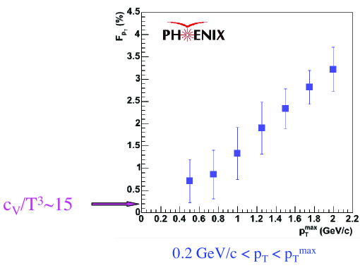
For RHIC at sN​N=200subscript𝑠𝑁𝑁200\sqrt{s_{NN}}=200 GeV, δ​ηFWHM=Β±3.5𝛿subscriptπœ‚FWHMplus-or-minus3.5\delta\eta_{\rm FWHM}=\pm 3.5Β PhobosWP , and the PHENIX acceptance was δ​ϕ=π𝛿italic-Ο•πœ‹\delta\phi=\pi, δ​η=Β±0.35π›Ώπœ‚plus-or-minus0.35\delta\eta=\pm 0.35, fcsubscript𝑓𝑐f_{c}=0.9 for pTβ‰₯0.2subscript𝑝𝑇0.2p_{T}\geq 0.2 GeV/c, resulting in ⟨Nt​o​t⟩/⟨n⟩=33delimited-⟨⟩subscriptπ‘π‘‘π‘œπ‘‘delimited-βŸ¨βŸ©π‘›33{\left<N_{tot}\right>/\left<n\right>}=33. From Fig.Β 4, FpTsubscript𝐹subscript𝑝𝑇F_{p_{T}} is of order 2% but most of that is due to jets, so the effect due to temperature fluctuations is <FpTabsentsubscript𝐹subscript𝑝𝑇<F_{p_{T}}, say 1%, so we obtain cv/T3>1/(33βˆ—0.01)=3subscript𝑐𝑣superscript𝑇31330.013c_{v}/T^{3}>1/(33*0.01)=3. This is to be compared to the Korus, et al.Β Korus , result of cv/T3=60Β±100subscript𝑐𝑣superscript𝑇3plus-or-minus60100c_{v}/T^{3}=60\pm 100Β MJTcalc from the NA49 data. Recall that Gavai, et al.,Β Gavai05 predict a value of 15 for cv/T3subscript𝑐𝑣superscript𝑇3c_{v}/T^{3}, which would correspond to a value of FpT=1%Γ—3/15=0.20%subscript𝐹subscript𝑝𝑇percent1315percent0.20F_{p_{T}}=1\%\times 3/15=0.20\% for the data in Fig.Β 4 (see Fig.Β 5).

Refer to caption
Figure 5: Gavai et al., predictionΒ Gavai05 compared to PHENIX measurement.

Perhaps this precision can be achieved by concentrating on the region pTmax≀0.6superscriptsubscript𝑝𝑇max0.6p_{T}^{\rm max}\leq 0.6 GeV/c, where jets have least effect. Also, as the present error is totally systematic due to run-by-run variation, there is hope that a substantial reduction should be possible.

V Conclusions

In central heavy ion collisions, the huge correlations in p-p collisions are washed outΒ Shuryak . The remaining correlations are: Jets; Bose-Einstein correlations; Hydrodynamic Flow. These correlations seem to saturate the present fluctuation measurements. No other sources of non-random fluctuations have been observed. This puts a severe constraint on the critical fluctuations that were expected for a sharp phase transition but is consistent with the present expectation from lattice QCD that the transition is a smooth crossover. In order to see the temperature fluctuations predicted by cv/T3≃15similar-to-or-equalssubscript𝑐𝑣superscript𝑇315c_{v}/T^{3}\simeq 15 in lattice gauge calculations, present sensitivity needs to be improved by an order of magnitude by removing the known sources of correlation and improving the measurement errors. An interesting check of whether temperature fluctuations, rather than the correlations noted above, produce the observed non-random fluctuations is provided by Eq.Β 10: for a pure ΟƒT2/⟨T⟩2subscriptsuperscript𝜎2𝑇superscriptdelimited-βŸ¨βŸ©π‘‡2\sigma^{2}_{T}/\left<T\right>^{2} fluctuation, FpTsubscript𝐹subscript𝑝𝑇F_{p_{T}} for a given centrality should increase linearly with the number of tracks measured (e.g. by increasing the solid angleβ€”PHENIX cf. STAR).

References

  • (1) Gavai RV, Gupta S, Mukherjee S (2005) The speed of sound and specific heat in the QCD plasma: hydrodynamics, fluctuations and conformal symmetry. Phys. Rev. D 71: 074013
  • (2) Korus R, Mrowczynski St, Rybczynski M, Wlodarczyk Z (2001) Transverse momentum fluctuations due to temperature variation in high-energy nuclear collisions. Phys. Rev. C 64: 054908
  • (3) Adler SS, et al., PHENIX Collaboration (2004) Identified charged particle spectra and yields in Au+Au collisions at sN​N=200subscript𝑠𝑁𝑁200\sqrt{s_{NN}}=200 GeV. Phys. Rev. C 69: 034909
  • (4) Stodolsky L (1995) Temperature Fluctuations in Multiparticle Production. Phys. Rev. Lett.Β  75: 1044–1045
  • (5) Shuryak EV (1998) Event-by-event analysis of heavy ion collisions and thermodynamical fluctuations. Phys. Lett. B 423: 9–14
  • (6) Stephanov M, Rajagopal K, Shuryak E (1999) Event-by-event fluctuations in heavy ion collisions and the QCD critical point. Phys. Rev. D 60: 114028
  • (7) Adler SS, et al., PHENIX Collaboration (2004) Measurement of Nonrandom Event-by-Event Fluctuations of Average Transverse Momentum in sN​N=200subscript𝑠𝑁𝑁200\sqrt{s_{NN}}=200 Au+Au and p+p𝑝𝑝p+p Collisions. Phys. Rev. Lett.Β  93: 092301
  • (8) Ferreiro EG, del Moral F, Pajares C (2004) Transverse momentum fluctuations and percolation of strings. Phys. Rev. C 69: 034901
  • (9) Back BB, et al., PHOBOS Collaboration (2005) The PHOBOS perspective on discoveries at RHIC. Nucl. Phys. A 757: 28–101
  • (10) Using the variable Ο•=ΟƒpT​FpT=2β€‹βŸ¨TβŸ©β€‹FpT=0.6Β±1.0italic-Ο•subscript𝜎subscript𝑝𝑇subscript𝐹subscript𝑝𝑇2delimited-βŸ¨βŸ©π‘‡subscript𝐹subscript𝑝𝑇plus-or-minus0.61.0\phi=\sigma_{p_{T}}F_{p_{T}}=\sqrt{2}\left<T\right>F_{p_{T}}=0.6\pm 1.0 MeV for T=180𝑇180T=180, from NA49, cited by Korus, et al.,Β Korus we find the value FpT=0.24%Β±0.39%subscript𝐹subscript𝑝𝑇plus-or-minuspercent0.24percent0.39F_{p_{T}}=0.24\%\pm 0.39\%. The values for ⟨n⟩=270delimited-βŸ¨βŸ©π‘›270\left<n\right>=270 and ⟨Nt​o​t⟩/⟨n⟩=1.5Γ—5delimited-⟨⟩subscriptπ‘π‘‘π‘œπ‘‘delimited-βŸ¨βŸ©π‘›1.55{\left<N_{tot}\right>/\left<n\right>}=1.5\times 5 also cited yield cv/T3=1/(7.5​FpT)=56Β±93subscript𝑐𝑣superscript𝑇317.5subscript𝐹subscript𝑝𝑇plus-or-minus5693c_{v}/T^{3}=1/(7.5F_{p_{T}})=56\pm 93 in agreement with the quoted value of 66Β±100plus-or-minus6610066\pm 100.