Optical Calibration For Jefferson Lab HKS Spectrometer

Abstract

In order to accept very forward angle scattering particles, Jefferson Lab HKS experiment uses an on-target zero degree dipole magnet. The usual spectrometer optics calibration procedure has to be modified due to this on-target field. This paper describes a new method to calibrate HKS spectrometer system. The simulation of the calibration procedure shows the required resolution can be achieved from initially inaccurate optical description.

1 Introduction

Jefferson Lab HKS experiment aims at obtaining high resolution hypernuclear spectroscopy (e.g., $\sim 400$ KeV FWHM for ${}^{12}_{\Lambda}$B) by $(e,e^{\prime}K)$ reaction (ref.[1]). It utilies CEBAF primary electron beam. The electroproduction provides a advantage over hadronic production mechanism because the momentum and position spread of the primary electron beam is significantly less than secondary hadron beams. The kaons are detected by High Resolution Kaon Spectrometer (HKS) with a momentum resolution of $2\times 10^{-4}$. In order to maximize hypernuclear yield, the target is placed just before a zero degree dipole magnet (Splitter). The field of the splitter is used to seperate scattered e’ from K⁺ and allow the spectrometer to accept both e’ and K⁺ from very forward angles.

To calculate hypernuclear excitation energies, we need to determine scattered kaon and electron momenta and angles. The kaon momentum is the dominant factor for the final missing mass resolution. In order to obtain the proposed missing mass resolution, it is important to optimize the spectrometer optics to get the required momentum and angle reconstruction resolution. This calibration procedure is complicated for HKS spectrometer Because of the existence of splitter magnet right after the target.

Table 1: required momentum and angle reconstruction resolution

K+ momentum	110 KeV/c (rms):1$\times 10^{-4}$
E’ momentum	120 KeV/c(rms):2$\times 10^{-4}$
K+ angle	2.9 mrad(rms)

The spectrometer optics can be conviniently expressed in a matrix formalism (ref.[2]), which is a set of polynimial coefficients related target angles and particle momentum to focal plane measurements. Conventionally, the method for calibrate matrix for angle reconstruction is by using a special designed collimator called sieve slit with a array of holes drilled onto metal template (ref.[2]). The sieve slit is mounted in front of the spectrometer entrance so all the particles passing through the holes will have defined incident angles.

But in the setup of HKS experiment, because target is inside the field of Splitter, the sieve slit plate can only be mounted on the Enge and HKS dipole entrance after the Splitter (fig.1). The particle trajectories are already bended by the splitter field before they pass through the sieve slit holes. Thus a hole of sieve slit no longer select a single, fixed angle. The usual way of angle reconstruction calibration has to be modified.

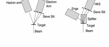
Figure 1: Schematic view of magnetic optical properties of normal double arm spectrometer system (left) and HKS spectrometer (right) with an on-target dipole magnet (Splitter).

For momentum calibration, because Enge, HKS two arms and the beam dump line are all coupled through splitter field, thus suitable kinematics setting for typical single arm momentum calibration (e.g., by production of carbon excited states) is difficult to implement.

In this paper a high precision optical calibration method for HKS spectrometer is described. The procedure can be applied to optical calibration of other magnet spectrometer system with on-target magnetic field. The optical calibration procedure will use the data from Enge and HKS sieve slit runs for angle reconstruction calibration and CH₂ target runs for momentum calibration. Before the experiment, the procedure has been tested by simulation with initial optics. The simulation is carried out by using measured field map of the spectrometer magnets and tracking particles through the field by program GEANT (ref. [3]). The calibration procedure for angle, momentum, kinematics reconstruction and beam raster correction will be described from Sec.1 to Sec.5 seperately. The iteration of these procedure is described in Sec.6. The simulation and result of the calibration procedure from is presented in sec.7, followed by a summary in section 8.

2 Sieve Slit Calibration

In HKS experiment, although the Splitter field smears the one to one correspondence between target angles and sieve slit hole position. The trajectory of a particle which passing through a given sieve slit hole and scattered from a point target is a functional of the paticle momentum and splitter optics. Thus with known splitter optics, the scattering angle can be expressed as a function of particle momentum and sieve slit hole position. The optics of Splitter can be obtained by measuring the field distribution of the magnet and tracking particles through the field by programs such as GEANT (ref.[3]). From the point of view of total integral of $Bdl$, the Splitter contribution is only $\sim 8$%, because the Splitter is just used to seperate particles. The contribution of field measurement error is negligible for target angle reconstruction.

Based on this observation, the sieve slit(SS) calibration procedure is:

1. Fit function $F_{s2t}$: target angles as a function of SS hole positions and particle momentum based on Splitter optics.

2. Separate events of the SS calibration run data hole by hole, thus determine corresponding SS hole center position for each event.

3. Using function $F_{s2t}$, calculate corrected target angles ($xptar$, $yptar$) for each event from SS center position and momentum.

4. Fit transfer matrix from focal plane to target: ($xfp$, $xpfp$, $yfp$, $ypfp$)$\longrightarrow$($xptar$, $yptar$).

A simulation of the SS calibration procedure with initial inaccurate Splitter, Enge optics reaches final resolution for e’ (Enge) target angles ($\sigma$): $xptar$: 1.8 mr, $yptar$: 1.1 mr, for kaon (HKS) angles: $xptar$: 0.4 mr, $yptar$: 2.4 mr.

3 Momentum Calibration

The method of HKS momentum calibration is making use of the known masses of $\Lambda$,$\Sigma^{0}$ hyperons and the narrow width of ${}^{12}_{\Lambda}$B hypernuclear ground state (ref.[4]). The hyperons is produced from hydrogens in the CH₂ foil (5 mm in thickness) The momentum reconstruction matrices for Enge and HKS arms are optimized simultaneously by minimizing the Chisquare defined as the sum of squared mass differences between the calculated mass and the PDB values. A Nonlinear Least Square method is used to optimize the matrices for electron arm and kaon arm simutaneously.

Although there is emulsion measurement of ${}^{12}_{\Lambda}$B GS binding energy at $11.37\pm 0.06$ MeV(ref.[5]), the associate statistical error and the composite nature ($2^{-}$/$1^{-}$) of the state may cause the peak center to deviate from this value (ref.[6]). So in the calibration process, the peak position is a adjustable parameter and the calibraion is carried out in a iterative way, the GS peak center is adjusted after each iteration according to the actual fitted position of calculated ${}^{12}_{\Lambda}$B GS distribution, until an minimum Chisquare is reached.

The procedure is:

1. Calculate missing mass using the existing angle matrix and the initial (un-calibrated) momentum matrix. From CH₂ target runs, select $\Lambda$,$\Sigma^{0}$ events, from Carbon target runs, select ${}^{12}_{\Lambda}$B GS events from a window located around the center of the missing mass peaks.

   Inside the 5mm thick CH₂ target, the energy loss and radiative processes are significant. It shifts the missing mass distributions and forms a tail. The width of the event window has to be selected appropriately, because a too wide window will dilute the sample with too many radiated events while a too narrow window will cause a insufficient statistics in the fitting.

2. Define Chisquare as the sum of squared mass differences $\Delta m_{i}^{2}$ between the calculated mass and the PDB values or the initial assumed ${}^{12}_{\Lambda}$B GS binding energy:

   $$\chi^{2}=\sum{w_{i}\Delta m_{i}^{2}}$$

   where $w_{i}$ is the relative weight of $\Lambda$,$\Sigma$ and ${}^{12}_{\Lambda}$B GS events.

3. $\chi^{2}$ is a function of missing mass $emiss$, thus a composite function of e’ and kaon momenta $\delta p_{e}$ and $\delta p_{k}$:

   $$\chi^{2}=f(emiss(\delta p_{e},\delta p_{k})$$

   Minimizing $\chi^{2}$ by by a Nonlinear Least Square method to optimize the Enge and HKS momentum reconstruction matrices(ref.[7]).

4. fit the actual peak center of the calculated ${}^{12}_{\Lambda}$B GS missing mass distribution. Using this value as the new ${}^{12}_{\Lambda}$B GS binding energy. Go back to first step. Iteration until an minimum Chisquare is reached.

4 Kinematics calibration

The purpose of kinematics calibration is to find the offsets of beam energy, Enge and HKS central momentum from nominal values. The method is also to use the known masses of $\Lambda$,$\Sigma^{0}$ and ${}^{12}_{\Lambda}$B ground state, same as momentum calibration. The $\chi^{2}$ is defined the same way as in momentum calibration. But for kinematics calibration, the $\chi^{2}$ is a function of beam energy offset $\Delta E_{e0}$, e’ central momentum offset $\Delta p_{e^{\prime}}$ and kaon momentum offset $\Delta p_{k}$, corresponding to the zero order terms in the momentum matrices. At correct offsets, this $\chi^{2}$ will be minimized.

If we define sum of kinematics offsets as:

$$\Delta p_{kin}=\Delta E_{e0}-\Delta p_{e^{\prime}}-\Delta p_{k}$$

.

The $\chi^{2}$ will dominantly depend on $\Delta p_{kin}$. Correct offsets can be found by scanning on $\Delta p_{kin}$ over all possible values to locate the minimum Chisquare.

5 Raster Correction

To avoid burning the CH₂ target, beam will be rastered 5mm$\times$5mm on the target by a pair of bending magnets. If the raster effect is ignored, a direct reconstruction with matrices obtained for point target gives much worse resolution, for example, the $\delta p$ resolution for HKS is $1.16\times 10^{-4}$(rms) without raster, it becomes $6.64\times 10^{-4}$ with 5mm$\times$5mm raster.

To do raster correction, the beam positions on target need to be determined by raster magnets X and Y current event by event. For rastered beam, The reconstructed target quantities can be expressed as functions of focal plane quantities and beam positions at target. It can be written as, for example:

$$\delta p=f(xfp,xpfp,yfp,ypfp)+g(xtar,ytar)$$

We seperated the dependence on beam positions from focal plane quantities so that the raster correction function $g$ depends only on beam position. It can be fitted from initial spectrometer optics. Even if the actual optics of the spectrometer system may deviate from the initial optics, its effect on raster correction function $g$ is negligible so we can still use the initial function form (fig.2 and fig.3).

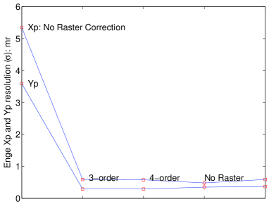
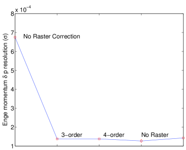
Figure 2: Comparison of Enge angle(left) and momentum(right) reconstruction resolution with rastered beam,with and without raster correction. Both resolutions are shown when the correction function $g$ fitted as a 3-order and 4-order polynomials. The rightmost point is the resolution after raster correction with wrong Enge optics.

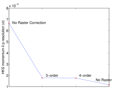
Figure 3: Comparison of HKS momentum reconstruction resolution with rastered beam,with and without raster correction.

6 Iterative Calibration

It is obvious that the individual calibration procedure mentioned above actually are correlated. For example, the calibration of target angles need the input of particle momentum while to extract missing mass, we need to know the scattering angle. Thus the individual calibraion procedures should be carried out in an iterative way until convergence is reached. The general procedure will be:

1. Separate Enge and HKS sieve slit calibration to obtain angle reconstruction matrices using original momentum reconstruction matrix.

2. Raster correction for CH₂ target data using existing raster correction matrix.

3. Kinematics calibration to find deviation of beam energy, Enge and HKS central momenta from their nominal values. The central angles of the spectrometers are not used in the missing mass calculation and they are not needed for fixed-angle spectrometer.

4. Two arm coupled momentum calibration to obtain momentum reconstruction matrix.

5. After getting the calibrated momentum matrix, go back to first step again to do SS calibration using the new momentum matrix. Iterate until best resolution is reached.

7 Simulation of the Calibration Procedure

Simulated events are used to test the calibration method. The simulation take account of target physics processes, spectrometer optics and detector resolution.

The simulation of target processes is adapted from SIMC (ref.[8]), a physics simulation program for Jefferson Lab Hall C basic equipment. The ionization energy loss, Bremsstrahlung, multiple scattering and beam spread effects are included in the simulation. The simulation uses 5mm thick CH₂ target and 0.1 g/cm² Carbon target.

Simulated events from target are send through The spectrometers. RAYTRACE (ref.[9]) is used to simulate events in the electron arm. A measured magnet field map is used to track particles through kaon arm by GEANT. Only optical properties (no physical processes) are considered in this step.

At focal plane of the spectrometers, the positions and angles are smeared according to detector resolution and multiple scattering. For Enge, the resolutions ($\sigma$) are: 86 $\mu$m (x), 0.7 mr(xp), 210 $\mu$m(y), 2.8 mr(yp). For HKS, they are: 160 $\mu$m (x and y), 0.33 mr (xp and yp).

The simulated focal plane events are then reconstructed back to the target using backward reconstruction matrix. The beam energy and particle momentum are corrected by the average energy loss in the target. The corrections are 0.4923 MeV (beam energy), 0.6015 MeV (e’ momentum), 0.4890 MeV (kaon momentum) for CH₂ target, 0.0820 MeV (beam energy), 0.1026 MeV (e’ momentum), 0.0866 MeV (kaon Momentum) for Carbon target.

The simulated $\Lambda$, $\Sigma^{0}$ and ${}^{12}_{\Lambda}$B missing mass spectra are shown in fig.4. The predicted $1^{-}$ state of ${}^{12}_{\Lambda}$B at 2.73 MeV is also included in the simulation for comparison. The quasi-free carbon background on CH₂ target is simulated with $\Lambda$ and $\Sigma^{0}$ events by a assumed S/B ratio of 6:1 under $\Lambda$ peak. The ${}^{12}_{\Lambda}$B GS has a missing mass resolution of 397 KeV (FWHM) with correct optics.

The simulated Enge focal plane sieve slit correlation patterns are shown in fig.5. Fig.6 shows the yfp vs. xfp correlations for each X-column of sieve slit holes.

The simulated HKS focal plane sieve slit patterns are shown in fig.7.

To test the calibration method by simulation, We intentionally use wrong spectrometer optics in reconstruction. The splitter field is changed from nominal value of 1.546 Tesla to 1.550 Tesla in forward simulation for e’ events, but still using the nominal reconstruction matrix in reconstruction. In addition, the beam energy, electron and kaon arm central momenta have offsets from nominal values, they are 1.2 MeV, -0.7 MeV and -0.9 MeV respectively. The missing mass distributions before the calibration is shown in fig. 8. The missing mass distributions after the calibration is in fig. 9. The width of the ${}^{12}_{\Lambda}$B GS improved from 1.56 MeV (FWHM) to 0.418 MeV (FWHM) after the calibration, and the center of GS peak is within 20 keV of the expected GS mass obtained by emulsion experiment.

Figure 4: Simulated $\Lambda$, $\Sigma^{0}$ and ${}^{12}_{\Lambda}$B missing mass spectra with Carbon QF background from CH₂ target.

Figure 5: Simulated Enge focal plane sieve slit correlation and hole patterns.

Figure 6: Simulated Enge focal plane $yfp$ vs. $xfp$ correlations for each X-column of sieve slit holes.

Figure 7: Simulated HKS focal plane sieve slit correlation and hole patterns.

Figure 8: Reconstructed $\Lambda$, $\Sigma^{0}$ and ${}^{12}_{\Lambda}$B missing mass spectra with wrong optics before the calibration.

Figure 9: Reconstructed $\Lambda$, $\Sigma^{0}$ and ${}^{12}_{\Lambda}$B missing mass spectra with optical matrices calibrated.

8 Summary

With the use of a dipole magnet on target, the normal spectrometer calibration procedure has to be modified. We have developed a new method for calibration of the reconstructions for target angle, momentum and kinematics. Starting from a initially inaccurate optics, by iteration of these calibration procedures, the spectrometer optics can be calibrated to the required resolution.

References

- [1] S.N.Nakamura, Nucl. Phys. A 754(2005) 421c.
- [2] E.A.J.M. Offermannn, C.W.De Jager and H. De. Vries, Nucl. Instr. and Meth. A262(1987) 298.
- [3] GEANT Manual v.3.21, Detector Description and Simulation Tool, CERN Program Long Write-up W5013 (1994).
- [4] Review of Particle Physics, S. Eidelman, et al., Phys. Lett. B592(2004) 1.
- [5] P. Dluzewski et al., Nucl. Phys. A484(1988) 520.
- [6] T. Motoba et al., Prog. Theor. Phys. Suppl., 117(1994) 123.
- [7] J.J. More, The Levenberg-Marquardt algorithm: Implementation and theory, In: Numerical Analysis, G.A. Watson (Ed.), Lecture Notes in Mathematics 630, Springer-Verlag, New York (1977).
- [8] J.Arrington, A-B-SIMC, Internal Jefferson Lab Hall C Tech Note.
- [9] S.B. Kowalski and H.A. Enge, Nucl. Instr. and Meth. A258(1987) 407.