Differential Cross Sections for $\gamma+p\rightarrow K^{+}+Y$ for $\Lambda$ and $\Sigma^{0}$ Hyperons.

Abstract

High-statistics cross sections for the reactions $\gamma+p\rightarrow K^{+}+\Lambda$ and $\gamma+p\rightarrow K^{+}+\Sigma^{0}$ have been measured using CLAS at Jefferson Lab for center-of-mass energies $W$ between 1.6 and 2.53 GeV, and for $-0.85<\cos\theta_{K^{+}}^{c.m.}<+0.95$. In the $K^{+}\Lambda$ channel we confirm a resonance-like structure near $W=1.9$ GeV at backward kaon angles. The position and width of this structure change with angle, indicating that more than one resonance is likely playing a role. The $K^{+}\Lambda$ channel at forward angles and all energies is well described by a $t$-channel scaling characteristic of Regge exchange, while the same scaling applied to the $K^{+}\Sigma^{0}$ channel is less successful. Several existing theoretical models are compared to the data, but none provide a good representation of the results.

I INTRODUCTION

We report on measurements of the photoproduction from the proton of two ground state hyperons, namely the reactions $\gamma+p\rightarrow K^{+}+\Lambda$ and $\gamma+p\rightarrow K^{+}+\Sigma^{0}$. Intermediate baryonic states in these reactions can be the $N^{*}$ resonances in the case of $\Lambda$ production, and $N^{*}$ or $\Delta$ resonances in the case of $\Sigma^{0}$ production. In either case one expects strange meson exchange in the $t$ channel and hyperon exchange in the $u$ channel. This is illustrated in Fig. 1. To unravel the production mechanism in these reactions, highly detailed measurements of as many observables as possible are needed.

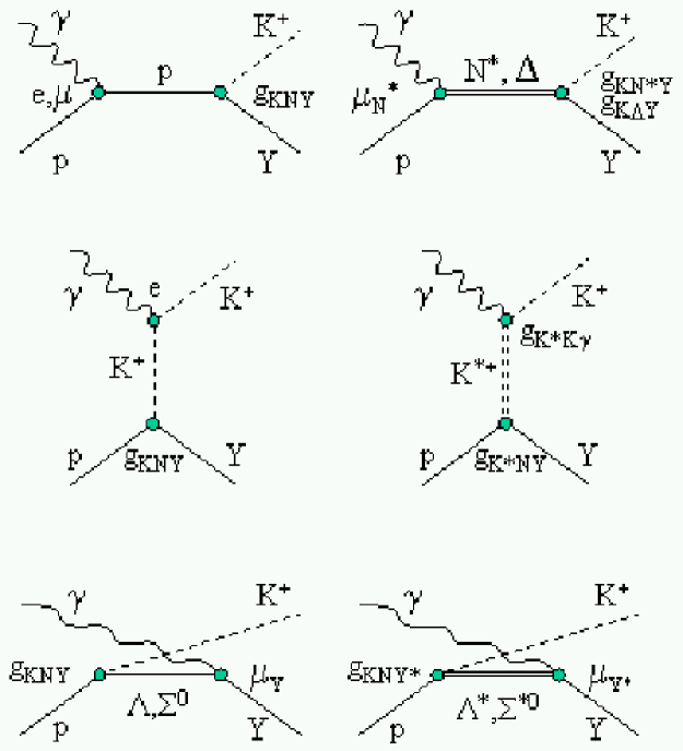
Figure 1: Representative tree-level diagrams illustrating $s-$ (top), $t-$ (middle), and $u-$ channel (bottom) exchanges. Born terms (left column), baryon resonance excitations (top right), and other exchanges (right middle, bottom) lead to production of $K^{+}Y$. Models differ in their electromagnetic transition moments ($\mu$’s),the strong couplings (g_MBB’s), and form factors, as well as the effects of channel couplings.

In this paper we present results for the differential cross sections, $d\sigma/d\cos(\theta_{K^{+}}^{c.m.})$, obtained with the CLAS system in Hall B at Jefferson Lab. Following our previous publication, Ref. mcnabb , these results are based on additional data accumulated by CLAS and use a different analysis technique. In another forthcoming paper we will present results for the beam-recoil double polarization observables, $C_{x}$ and $C_{z}$, for the same reactions obtained from the same data set.

The main motivation for this work was to provide data to investigate the spectrum of non-strange ($N^{*}$ and $\Delta$) baryon resonances above the strangeness-production threshold at $W=\sqrt{s}=1.6$ GeV. Between this threshold and the upper limit of our data set, at $W=2.53$ GeV, many baryon resonances are predicted by quark models cap , but relatively few are clearly established pdg . These resonances are broad and overlapping, making partial wave analysis challenging, but it is also possible that some dynamical aspect of hadronic structure may act to restrict the quark models’ spectrum of states to something closer to what has already been established klempt . This is the so-called “missing resonance” problem. While the branching fractions of most high-mass resonances to $KY$ final states are expected to be small (cross sections $\sim 1~{}\mu b$) compared to three-body modes such as $\pi\pi\ N$ ($\sim 100~{}\mu b$), the study of these decays do have advantages. First, two-body final states are often easier to analyze than three-body final states. Second, couplings of nucleon resonances to $KY$ final states will differ from coupling to $\pi N$, $\eta N$, or $\pi\pi N$ final states cap . Thus, one can hope that this alternate light cast on the baryon resonance spectrum may emphasize resonances not otherwise revealed. Some “missing” resonances may only be “hidden” when sought in more well-studied reaction channels.

The $\Lambda$ and $\Sigma^{0}$ hyperons have isospin 0 and 1, respectively, and so intermediate baryonic states leading to the production of $\Lambda$’s can only have isospin 1/2 ($N^{*}$ only), whereas for the $\Sigma^{0}$’s, intermediate states with both isospin 1/2 and 3/2 ($N^{*}$ or $\Delta$) can contribute. Thus, simultaneous study of these reactions provides a kind of isospin selectivity of the sort used in comparing $\eta$ and $\pi$ photoproduction reactions. To date, however, the PDG compilation pdg gives poorly-known $K\Lambda$ couplings for only five well-established resonances, and no $K\Sigma$ couplings for any resonances. The most widely-available model calculation of the $K\Lambda$ photoproduction, the Kaon-MAID code maid , includes a mere three well-established $N^{*}$ states: the $S_{11}(1650)$, the $P_{11}(1710)$, and the $P_{13}(1720)$. Thus, it is timely and interesting to have additional good-quality photoproduction data of these channels to see what additional resonance formation and decay information can be obtained.

Section II of this paper discusses briefly the reaction models that will be compared with the present data. Section III discusses the experimental setup of the CLAS system for this experiment. The steps taken to obtain the cross sections from the raw data are discussed in Section IV. Section V presents the results for the measured angular distributions and $W$-dependence of the cross sections. In Section VI we discuss the results in light of previous measurements, and in relation to several previously-published reaction models. We also show how the data can be parameterized in terms of $t$-channel scaling using a simple Regge-based picture, and in terms of simple Legendre polynomials. In Section VII we recapitulate the main results.

II THEORETICAL MODELS

The results in this experiment will be compared to model calculations that fall into two classes: tree-level Effective Lagrangian models and Reggeized meson exchange models. Effective Lagrangian models evaluate tree-level Feynman diagrams as in Fig. 1, including resonant and non-resonant exchanges of baryons and mesons. A complete description of the physics processes will require taking into account all possible channels which could couple to the one being measured, but the advantages of the tree-level approach are to limit complexity and to identify the dominant trends. In the one-channel tree-level approach, some tens of parameters (in particular, the couplings of the non-strange baryon resonances to the hyperon-kaon systems) must be fixed by fitting to data, since they are poorly known from other sources. An alternative approach is to use no baryon resonance terms and instead model the cross sections in a Reggeized meson exchange picture. While this is not expected to reproduce the results in detail, it will show where the high-energy phenomenology of $t$-channel dominance blends into the nucleon resonance region picture.

For $K^{+}\Lambda$ production, the model of Mart and Bennhold mart has four baryon resonance contributions. Near threshold, the steep rise of the cross section is accounted for with the $N^{*}$ states $S_{11}(1650)$, the $P_{11}(1710)$, and $P_{13}(1720)$. To explain the broad cross-section bump in the mass range above these resonances, they introduced the $D_{13}(1895)$ resonance that was predicted in the relativized quark models of Capstick and Roberts cap and Löring, Metsch, and Petry loring to have especially strong coupling to the $K^{+}\Lambda$ channel. In addition, the higher mass region has contributions, in this model, from the exchange of vector $K^{*}(892)$ and pseudovector $K_{1}(1270)$ mesons. The hadronic form factors, cutoff masses, and the prescription for enforcing gauge invariance were elements of the model for which specific choices were made. The content of this model is embedded in the Kaon-MAID code maid which was used for the comparisons in this paper. This model was tuned to results from the experiment at Bonn/SAPHIR bonn1 , and offers a fair description of those results.

On the other hand, analysis by Saghai et al. sag using the same data set showed that, by tuning the background processes involved, the need for the extra resonance was removed. Janssen et al. jan ; jan_a showed that the same data set was not complete enough to make firm statements since models with and without the presence of a hypothesized $N^{*}(1895)D_{13}$ resulted in equally good fits to data. A subsequent analysis  ireland , which also fitted calculations to photon beam asymmetry measurements from SPring-8 zegers and electroproduction data measured at Jefferson Lab mohring , indicated weak evidence for one or more of $S_{11}$, $P_{11}$, $P_{13}$, or $D_{13}(1895)$, with the $P_{11}$ solution giving the best fit. The conclusion was that a more comprehensive data set would be required to make further progress.

More elaborate model calculations have been undertaken in which channel coupling is considered, in addition to the tree-level approaches mentioned above. Penner and Mosel penner found fair agreement for the $K^{+}\Lambda$ data without invoking a new $D_{13}$ structure. Chiang et al. chiang showed that coupled channel effects are significant at the $20\%$ level in the total cross sections when including pionic final states. Shklyar, Lenske, and Mosel shklyar used a unitary coupled-channel effective Lagrangian model applied to $\pi$ and $\gamma$ -induced reactions to find dominant resonant contributions from $S_{11}(1650)$, $P_{13}(1720)$, and $P_{13}(1895)$ states, but not from $P_{11}(1710)$ or $D_{13}(1895)$. This conclusion was true despite the discrepancies between previous data from CLAS mcnabb and SAPHIR bonn2 . Recently, Sarantsev et al. sarantsev did a phenomenological multi-channel fit for $K\Lambda$, $K\Sigma$, as well as $\pi$ and $\eta$ photoproduction data. They found fairly strong evidence for a $P_{11}$ at 1840 MeV and two $D_{13}$ states at 1870 and 2170 MeV. Even better quality $KY$ data such as we are presenting here are needed to solidify these conclusions. We will not compare the present results to those models in this paper, however.

While it is to be expected that $s$-channel resonance structure is a significant component of the $K^{+}\Lambda$ and $K^{+}\Sigma^{0}$ reaction mechanisms, it is instructive to compare to a model that has no such content at all. The model of Guidal, Laget, and Vanderhaeghen lag1 ; lag2 is such a model, in which the exchanges are restricted to two linear Regge trajectories corresponding to the vector $K^{*}$ and the pseudovector $K_{1}$. The model was fit to higher-energy photoproduction data where there is little doubt of the dominance of these exchanges. In this paper, we extend that model into the resonance region in order to make a critical comparison.

III EXPERIMENTAL SETUP

Differential cross section data were obtained with the CLAS system in Hall B at the Thomas Jefferson National Accelerator Facility. Electron beam energies of 2.4 and 3.1 GeV contributed to the data set, each of typically 10 nA current. Real photons were produced via bremsstrahlung from a $1\times 10^{-4}$ radiation length gold radiator and “tagged” using the recoiling electrons analyzed in a dipole magnet and scintillator hodoscopes tagger . The energy tagging range was from 20% to 95% of the beam endpoint energy, and the integrated rate of tagged photons was typically $5\times 10^{6}$ /sec. Using the tagger and the accelerator RF signal, photon timing at the physics target was defined with an rms precision of 180 psec. The useful energy range for this experiment was from the strangeness-production threshold at $E_{\gamma}=0.911$ GeV ($W$ = 1.61 GeV) up to 2.95 GeV ($W$ = 2.53 GeV). In this range, the tagger resolution was typically 5 MeV, set by the size of the hodoscope elements, but the data were analyzed in bins of 25 MeV photon energy to be commensurate with any energy-dependent structure expected in the hadronic cross sections. The centroids of these bins were adjusted in the analysis by between $-6$ and $+5$ MeV to compensate for mechanical sag of the hodoscope array measured by kinematically fitting $p(\gamma,p\pi^{+}\pi^{-})$ data; hence our final results are given in unequal energy steps.

The physics target consisted of a 17.9 cm long liquid hydrogen cell of diameter 4.0 cm. Temperature and pressure were monitored continuously to determine the density to 0.3% precision. The target cell was surrounded by a set of six 3 mm thick scintillators to help define the starting time for particle tracks leaving the target, though actually the timing given by the photon tagger was used to define the event times.

The CLAS system, described in detail elsewhere clas0 , consisted of a toroidal magnetic field, with drift chamber tracking of charged particles. The overall geometry was six-fold symmetric viewed along the beam line. Particles could be tracked from $8^{\circ}$ to $140^{\circ}$ in laboratory polar angle, and over about $80\%$ of $2\pi$ in the azimuthal direction. Outside the magnetic field region a set of 288 scintillators was used for triggering and for later particle identification using the time-of-flight technique. The momentum resolution of the system was $\approx 0.5\%$, with variations due to multiple scattering and tracking resolution considerations. The low-momentum cut-off was set in the analysis at 200 MeV/c. Other components of the CLAS system, such as the electromagnetic calorimeter and the Cerenkov counters, were not used for these measurements.

The event trigger required an electron signal from the photon tagger, and at least one charged-track coincidence between the time-of-flight ‘Start’ counters near the target and the time-of-flight ‘Stop’ counters surrounding the drift chambers. The photon tagger signal consisted of the OR of coincidences among hits in a two-plane hodoscope, which had 61 timing scintillators in coincidence with their matching energy-defining scintillators. The charged-track trigger in CLAS was a coincidence of six OR’d start counter elements and the OR of the outer time-of-flight scintillators. Events were accumulated at the rate of $\sim 2500$ hadronic events per second, though only a sub-percent fraction of these events contained the kaons and hyperons of interest for the present analysis.

IV DATA ANALYSIS

IV.1 Data and event selection

The data used in this experiment were obtained in late 1999 as part of the CLAS “g1c” data taking period. Since the electronic trigger was loose, data for several photoproduction studies were contained in the data set. Off-line calibration was performed to align the timing spectra of the elements of the photon tagger, the six elements of the start counter, and the 288 elements of the time-of-flight (TOF) counters. Drift-time calibrations were made for the 18 drift chamber packages. Pulse height calibrations and timing-walk corrections were made for the time-of-flight counters. The raw data were then processed to reconstruct tracks in the drift chambers and to associate them with hits in the time-of-flight counters.

IV.2 Particle Identification

Kaon, proton, and pion tracks were separated using momentum and time-of-flight measurements. The momentum, $\vec{p}$, of each track was measured directly via track reconstruction through the CLAS magnetic field; this measurement also gave the path length, $d$, from the reaction vertex to the time-of-flight counter hit by the track. The starting time of the track was determined by projecting the tagger signal time, synchronized with the accelerator RF timing, to the reaction vertex inside the hydrogen target. The stopping time was determined by the element hit in the array of TOF scintillators. The difference, $T$, between these two times was the measured time of flight, which in CLAS could range between about 4 and 100 nsec. From $T$ the speed, $\beta$, could be obtained as $\beta=d/(cT)$. The mass, $m_{x}$, was then computed according to $m_{x}=\sqrt{1-\beta^{2}}\times pT/d$. In CLAS, the dominant mass uncertainty in this situation came from the time-of-flight resolution, $\delta T$. $\delta T$ was independent of particle momentum, so particle selection based on time of flight was largely independent of momentum as well. For kaon identification we used the time-of-flight difference technique, where the measured time, $T$, of the track was compared to the expected time, $T_{h}$, for a hadron of mass $m_{h}$ and momentum $p$. For a hypothesized value of $m_{h}$ we can define $\Delta tof=T-T_{h}$ and write

$$\Delta tof=T\left(1-\sqrt{\frac{(m_{h}c)^{2}+p^{2}}{(m_{x}c)^{2}+p^{2}}}\right).$$ (1)

Figure 2 shows an example of such a time difference spectrum when we took $m_{h}$ to be the kaon mass. The candidate kaon tracks were selected using a $\pm 1$ nsec cut centered at zero. Pion and proton bands are well separated from the kaons up to 1 and 2 GeV, respectively. A crossing band due to a badly-calibrated detector element is shown for illustration; such tracks were later rejected by removing the detector element and/or by the kinematic cuts and fits applied later. Above 1 GeV some pions leak into the set of candidate kaon tracks. These were rejected by subsequent event reconstruction cuts and by background rejection fitting. Protons were identified using a similar $\Delta tof$ correlation but with looser cuts due to the straggling effects which broadened the distribution.

Photons matching the hadronic tracks in CLAS were selected using the time difference between the hadronic track projected back to the event vertex and the photon tagger time projected forward to the event vertex. Figure 3 shows such a spectrum, which illustrates the presence of random coincidences between the photons and the hadronic tracks. The 2 nsec RF time structure of the accelerator is clearly seen. A $\pm 1.0$ nsec cut was used to reject out-of-time combinations. In-time accidentals under the central peak were treated as potentially-correct photons, and such particle-photon combinations were retained in the analysis. Since ambiguous photons were generally widely separated in energy, the $(\gamma,K^{+})$ missing mass for incorrect combinations fell into the broad background under the hyperons, and were then rejected at the peak-fitting stage of the analysis discussed below.

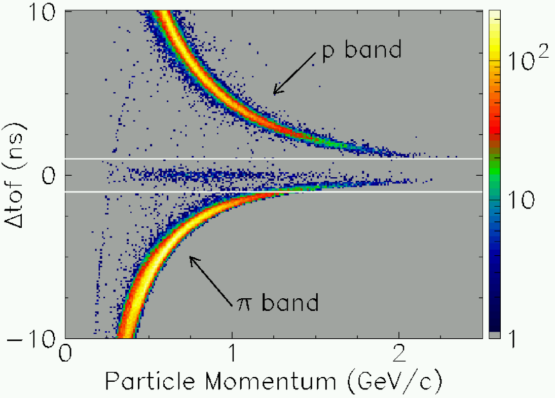
Figure 2: (Color online) Time-of-flight difference spectrum for a sample of tracks, assuming the mass of the particle is that of a kaon. White lines indicate the cut limits for selecting kaons in a time window of $\pm 1.0$ nsec. Note the logarithmic scale on the intensity axis.

Figure 3: Time difference between photon tagger time and target start counter time showing the peak at zero of good matches between the photons and the hadrons at the event vertex in CLAS. Coincidences due to hadrons mismatched to random photons in the tagger show the 2 nsec bunch structure of CEBAF.

In this analysis we demanded detection of positive kaons and protons. Negative pions from $\Lambda$ decay or photons from $\Sigma^{0}$ decay were not required. Fiducial cuts were applied in track angle and momentum to restrict events to the well-described portions of the detector. This included removal of 9 out of 288 time-of-flight elements due to poor timing properties. Corrections were applied for the mean energy losses of kaons and protons as they passed through the production target, target walls, beam pipe, and air. The nominal CLAS momentum reconstruction algorithms were found to provide sufficient hyperon mass resolution (see below) that no higher-order momentum corrections were applied.

A missing mass cut was applied to $p(\gamma,K^{+}p)\pi^{-}(\gamma)$ to select events consistent with a missing pion and (for the $\Sigma^{0}$) a missing photon. The losses incurred by this cut due to multiple scattering effects on the part of the kaons and protons were studied in the real data and in Monte Carlo. The estimated residual uncertainty due to the cut and its compensation via the acceptance calculation was $1\%-2\%$.

IV.3 Yield of hyperons

The extraction of kaon yields in each bin of photon energy and kaon angle depended on fits to the missing mass spectrum given by $p(\gamma,K^{+})Y$. When integrating over all of our 3.1 GeV data, for all energies and angles, the resulting missing mass spectrum is shown in Fig. 4. This figure illustrates that the overall missing mass resolution of the system was $\sigma=8.9$ MeV for the $\Lambda$ and $\sigma=8.2$ MeV for the $\Sigma^{0}$. The overall resolution averaged 6.3 MeV in the 2.4 GeV data set, where all the average momenta were lower. However, the width of the peaks and the extent of the background to be removed from under the peaks via fitting varied substantially across the measured range of energy and angle, so a careful fitting procedure was needed to obtain well-controlled hyperon yields.

Figure 4: Hyperon spectrum via missing mass using the photon and detected kaon, integrated over all kaon angles and photon energies using a 3.1 GeV endpoint energy.

The main source of background in the hyperon mass spectra was due to events where the kaons were actually mis-identified pions. The yields of $\Lambda$ and $\Sigma^{0}$ hyperons were obtained using lineshape fits to missing-mass spectra in each of over 1,450 kinematic bins of photon energy and kaon angle. The data were binned in 25 MeV steps in $E_{\gamma}$ and in 18 bins of kaon center-of-mass (c.m.) angle, $\cos(\theta_{K^{+}}^{c.m.})$, centered in steps of 0.1 between $-0.8$ and $+0.9$.

Typical hyperon yield fits of $p(\gamma,K^{+})Y$ for the middle of the photon energy range are shown in Fig. 5. The fits were performed in two passes. In the first pass, events for all kaon center-of-mass angles were summed together. These first fits served to determine and fix the centroids and widths of the Gaussian peaks for the two hyperons. These were 7 to 9 parameter fits, depending on the background model employed. A log-likelihood fitting algorithm was used. The background was modeled as polynomials of order up to 2 (quadratic). In the second pass, fits were made with 3 to 5 parameters for the yields in each kaon angle bin, allowing only the integrated counts of the peaks to vary in addition to the background parameters. The two-pass method was used to stabilize fits of low-yield bins at low photon energy and backward kaon angle. Acceptable fits all had $\chi^{2}$ per degree of freedom of less than 2.0.

Background parameterizations that were a simple constant or a sloped line were sufficient to yield good fits over most of the kinematic range. At more forward kaon angles the effect of background due to mis-identified pions increased and the quadratic fits generally gave the best results. Above $E_{\gamma}=2.3$ GeV the momentum resolution of CLAS broadened to the degree that the forward-angle quadratic fits became less stable, so the linear fits were preferred. This led to an extra estimated systematic uncertainty of 10% on both the forward-angle differential and total cross sections above this energy. In some low-yield back-angle bins, where no good fits were obtained, side-band subtraction was used to determine the yield.

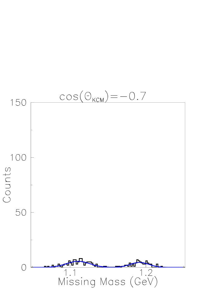
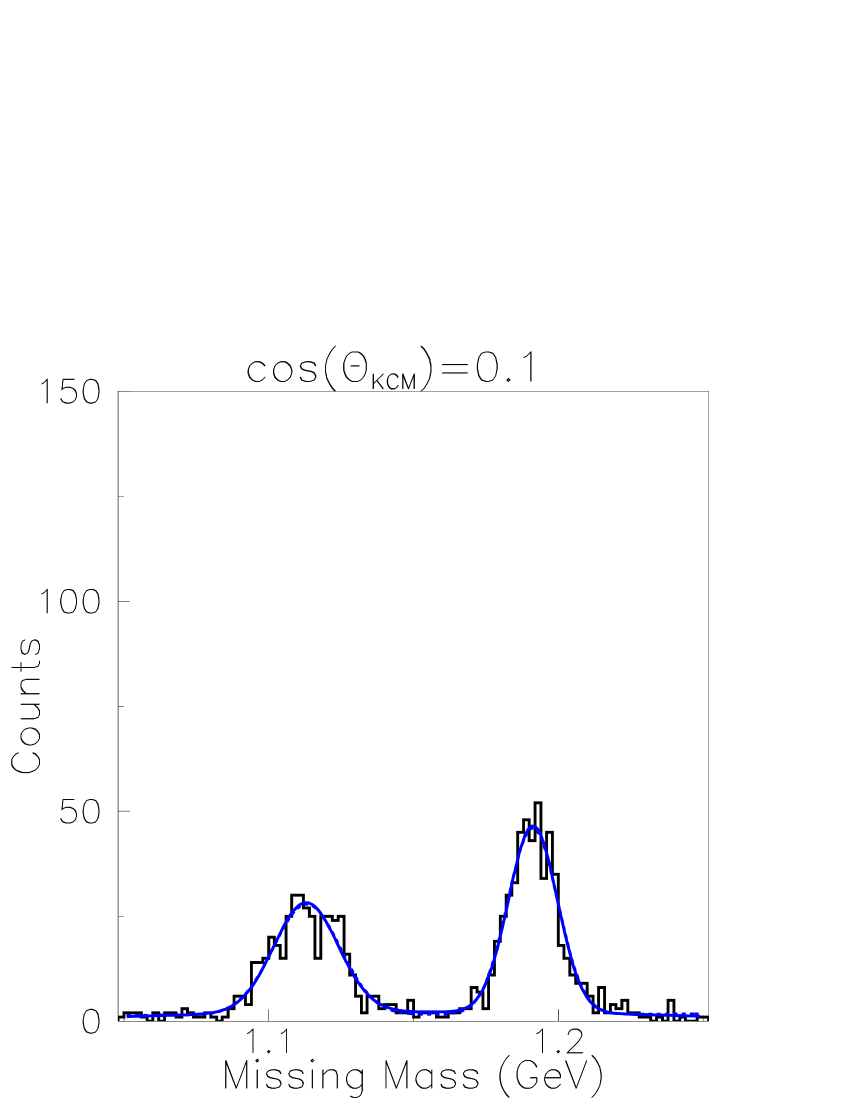
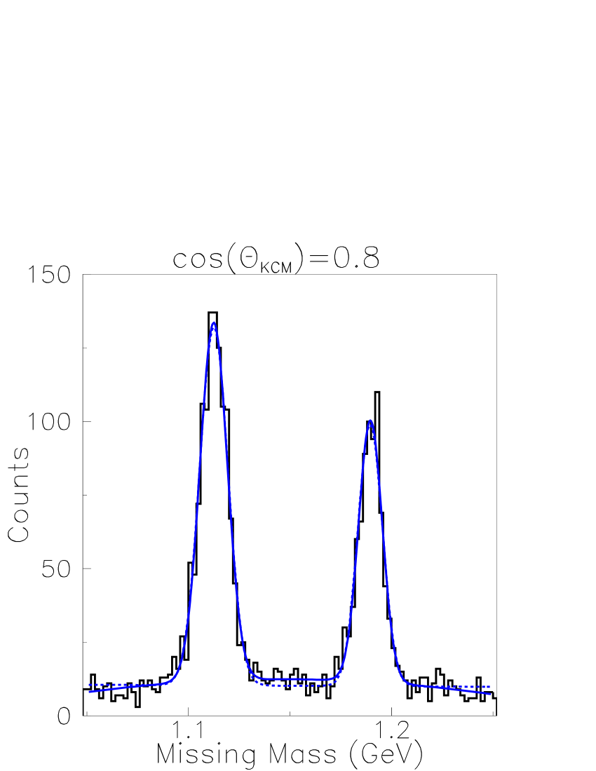
Figure 5: Sample missing mass fits used for the determination of hyperon yields at $E_{\gamma}=1.825$ GeV and for three representative $K^{+}$ angles: $\cos(\theta_{K^{+}}^{c.m.})=-0.7,+0.1,+0.8$. The fits to different orders of polynomial background are nearly indistinguishable: solid lines for quadratic and dashed lines for linear.

The final cross sections were based on the following numbers of fully reconstructed events: from the 2.4 and the 3.1 GeV data sets we had 236,260 and 325,792 $K^{+}\Lambda$ events, respectively, and 169,796 and 269,216 $K^{+}\Sigma^{0}$ events, respectively.

IV.4 Acceptance calculation

The acceptance and efficiency were modeled using a CLAS-standard GEANT-based simulation code (“GSIM”). Events were initially modeled using a phase space distribution for $\gamma+p\rightarrow K^{+}+Y$. The GSIM code simulated the events in the CLAS detector at the level of ADC and TDC hits in the scintillators and drift time information in the tracking chambers. The events were further fine-tuned such that the time distributions in the TDC’s accurately matched the actual data using another well-tested CLAS software package (“GPP”). These simulated events were then processed through the same analysis codes as the real data, and thus the acceptance was computed in each kinematic bin. Dead regions of the drift chambers were removed both from the real data and from the simulated data during track reconstruction (“A1C”). Detector efficiency was simultaneously accounted for through the simulation: sources of inefficiency included track reconstruction failures and time-of-flight paddle removals. The only particle background in this physics Monte Carlo was due to particle decays, especially the kaons, and multiple scattering effects. Thus, we relied on the yield extractions discussed earlier to remove background due to mis-identified pions or protons.

The effect of using a phase-space event generator to compute the acceptance, $\eta_{P.S.}$, was studied by using the fits to the angular distributions presented in Section V.1 to regenerate the acceptance, $\eta_{Data}$, with an improved representation of the reactions. Since these cross sections vary quite slowly with angle, and since the kinematic bins were each small on the scale of these variations, no large effects were to be expected. We found agreement between the two acceptance models at the level of $0.25\%$ $rms$ over essentially the whole of the kinematic space, consistent with the statistical variations of the simulations. The exception was in the forward-most angle bin ($0.85<\cos(\theta_{K^{+}}^{c.m.})<0.95$) for both hyperons. There, because of the extrapolation of the analysis into CLAS’s forward acceptance hole, the ratio of acceptances $\eta_{Data}/\eta_{P.S.}$ dropped from 1.0 to 0.85 over the range $E_{\gamma}\sim 1.75$ GeV to $E_{\gamma}\sim 2.90$ GeV. Theoretical models of the behavior of the cross section in the very forward direction differ strongly, as shown later, so it was not known whether a “flat” or a “forward-peaked” or a “forward-dipped” acceptance model was more accurate. Thus, the forward-most angle results at $\cos(\theta_{K^{+}}^{c.m.})=+.9$ have an additional systematic uncertainty on the cross section which is, on the average, $\pm 8\%$.

A sample of the acceptances computed for CLAS for these reactions is shown in Fig. 6. It was largest at mid to forward kaon angles and at higher photon energies. The maximum acceptance was about $22\%$ for $K^{+}\Lambda$ and $23\%$ for $K^{+}\Sigma^{0}$. A lower cut-off was applied, such that the smallest allowed acceptance in the experiment was $0.5\%$. For each hyperon, 10 million events were generated at each beam endpoint energy. Non-uniformities in the distribution arise from the effects of detector element removals and track reconstruction efficiencies. Since the kinematics of the two hyperon reactions are very similar, the acceptance function for the $\Sigma^{0}$ looked very similar, apart from the higher production threshold.

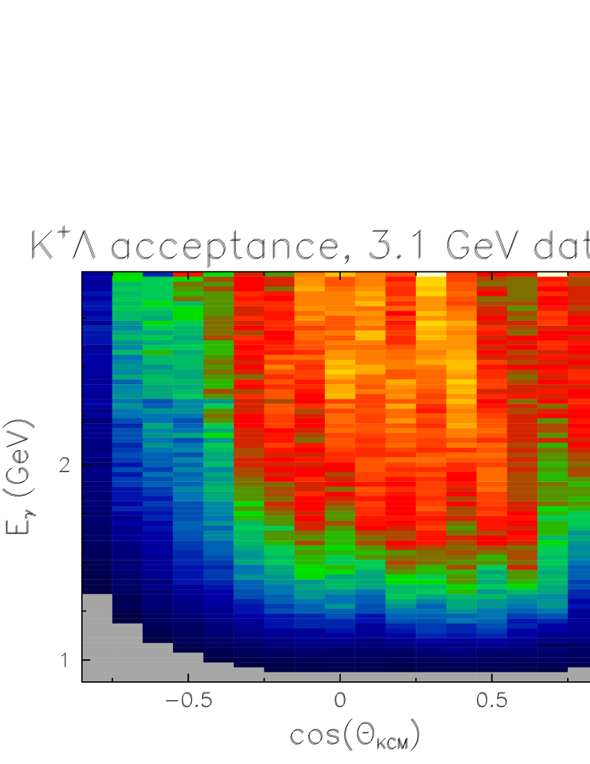
Figure 6: (Color online) Computed CLAS acceptance for the $E_{\gamma}=3.1$ GeV data set for the $\gamma+p\rightarrow K^{+}+\Lambda$ reaction. The scale on the right gives the value of the acceptance for each kinematic bin.

IV.5 Photon flux

The number of photons striking the target was computed from the measured rate of electrons detected at the tagger hodoscope. TDC spectra of the tagger elements recorded the hits of electrons in a 150 nsec time range around each event. This flux was scaled and integrated in ten-second intervals. After statistical corrections for multiple hits and electronic live time, the flux was summed over whole runs. The fine granularity of the tagging system was grouped into bins of 25 MeV in photon energy.

Photon losses in the beam line due to tagger acceptance, beam collimation, and thin windows were determined using a separate total-absorption counter downstream of CLAS. This low-rate lead glass detector was periodically put in the beam line to monitor the tagging efficiency. For the 2.4 GeV data set the average efficiency for tagging photons was 78%, and the stability of this efficiency, which was measured periodically throughout the data taking period, was $\pm 0.5\%$.

By taking data at 2.4 and 3.1 GeV endpoint energies it was possible to test the flux normalization of many elements of the tagging system, as discussed in the next section. At energies above $E_{\gamma}=2.325$ GeV the two data sets no longer overlapped, however, and defective electronics in a few channels of the tagger led to a gap in our final spectra. Bins at $E_{\gamma}=$ 2.375 and 2.400 GeV were removed because of this.

IV.6 Systematic uncertainties

The 2.4 and 3.1 GeV photon beam endpoint data sets were compared to investigate variations in the photon tagger efficiency. The photon-normalized yield of particles at any given energy had to be independent of bremsstrahlung endpoint energy, so consistency of this quantity tested stability of the electronics. Localized regions of tagger inefficiency “moved” in photon energy when the endpoint energy changed. We took the higher normalized yield between the two data sets as the correct one. Localized regions of high inefficiency were found in the 3.1 GeV data set at 1.1, 1.4, and 1.8 GeV; in those regions we made corrections of up to 50% in one data set to compensate for tagger efficiency losses in the other. Much smaller corrections ($\sim 3\%$) were made at other energies. The absolute uncertainty on these corrections was estimated to be $\pm 3\%$.

As a check on our results, the $p(\gamma,\pi^{+})n$ cross section was measured using the same analysis chain, as far as possible, as the $p(\gamma,K^{+})Y$ data. The same procedure was also used to generate the acceptance for the $p(\gamma,\pi^{+})n$ cross sections used to check the whole analysis process, except that the SAID code was used to generate the initial events. Figure 7 shows the pion cross section measured in this analysis as a function of $W$ for a mid-range c.m. pion angle. The CLAS pion cross section was found to be in fair agreement with the SAID said parameterization of the world’s data between $W=1.6$ and $2.1$ GeV, albeit lower by an average scale factor of 0.95. As a function of pion center of mass angle, the CLAS to SAID ratio was $\sim 1.0$ at back angles and $\sim.92$ at forward angles. Thus the pion results indicate a possible systematic error in the acceptance calculation at the level of $\pm 3\%$, apart from the average scale factor. The absolute accuracy of the pion cross sections, as parameterized by SAID over the range of comparison we used, is similar to this. Therefore, we chose not to make a renormalization of our results to the average pion cross sections. The results presented in this paper are on an absolute scale. The kaon analysis was not identical to the pion analysis, since the kaon decay corrections are much larger in the former case, and since the final kaon analysis included detection of the proton from the hyperon decays. Hence, it was difficult to translate the systematic trends in our pion results compared to SAID to the kaon results presented here. However, based on the comparison to the pion data analysis, we estimated the overall systematic uncertainty in our kaon cross section to be less than $\pm 7\%$. This was the largest single contribution to our cross section systematic uncertainty.

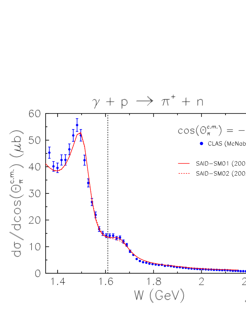
Figure 7: CLAS differential cross section as a function of $W$ for $\gamma+p\rightarrow\pi^{+}+n$. Shown for comparison are two versions of the SAID parameterization of world pion data. They are essentially indistinguishable. The vertical dotted line is the strangeness production threshold.

The analysis of this experiment was done twice, in largely independent ways. The first analysis john ; mcnabb computed cross sections based on detection of the kaon alone, or $p(\gamma,K^{+})Y$. Starting from the same data set, the second analysis bradford detected the kaon and the proton for each event, or $p(\gamma,K^{+}p)\pi^{-}(\gamma)$, where the $\pi^{-}$ (and the possible $\gamma$ from $\Sigma^{0}$ decay) were ignored. Particle identification and acceptances were developed independently. For the results presented here, the first analysis was revised to take into account more advanced modeling of the CLAS detector in the acceptance; both analyses used the standard CLAS GEANT package for computing acceptances. The same flux normalization procedures were used. The first analysis used only data from the 2.4 GeV endpoint data set, while the second analysis also included data from 3.1 GeV endpoint. Consistency checks were then made between the two analyses. Results for the final cross sections from the two studies were in very good agreement across the full range of energies and angles where they overlapped. Isolated differences of $\sim 5\%$ in small ranges of angle were attributed to details of the acceptance modeling. By comparing the acceptances developed over the course of the $p(\gamma,K^{+})Y$ studies, we estimated that average systematic uncertainty across the kinematics of the experiment was $\pm 2.7\%$, arising from variations in the implementation of the detector model and the track-reconstruction algorithms.

On the energy axis, our results are precise to $\pm 2$ MeV. This systematic uncertainty arises from an energy bin centering correction that was applied to each data point due to the calibration of the photon tagger. In an independent study, kinematic fitting to the reaction $p(\gamma,p\pi^{+}\pi^{-})$ showed that the CLAS tagger and the photon beam were mismatched by up to $\pm 10$ MeV due to mechanical effects in the structure of the tagger. The correction shifted the centroids of each energy bin by an amount estimated to be precise as stated above. The indirect effect that this centroid shift had on the acceptance of CLAS was considered negligible, since the cross sections vary slowly in energy and the energy bins for the results are 25 MeV wide.

The estimated systematic uncertainties discussed above were combined with contributions due to particle yield extraction $(3.6\%)$, photon attenuation in the beam line $(0.2\%)$, target density uncertainty $(0.14\%)$, and target length uncertainty $(0.28\%)$. This led to an estimate of the global scale uncertainty of $\pm 8\%$. Due to additional systematic uncertainty about extrapolation of the data to zero degrees, the forward-most angle bin above $E_{\gamma}=1.75$ GeV has an overall uncertainty of $\pm 11\%$.

V RESULTS

V.1 Angular Distributions

Since the differential cross sections in this measurement are symmetric in the azimuthal angle $\phi$, we present the results in the partially integrated form

$$\frac{d\sigma}{d(\cos\theta_{K^{+}}^{c.m.})}=2\pi\frac{d\sigma}{d\Omega}$$ (2)

since this also puts the values on a convenient scale of order $1~{}\mu b$.

The angular distribution results for the reaction $\gamma+p\rightarrow K^{+}+\Lambda$ are shown in Fig. 8. The results are shown as a function of $\cos(\theta_{K^{+}}^{c.m.})$ for 79 bins in $W$. The step sizes in $W$ were determined by the 25-MeV step size in the nominal photon energy, $E_{\gamma}$, at which the cross sections were extracted, together with a few-MeV correction for tagger re-calibration. There are 18 bins in $\cos(\theta_{K^{+}}^{c.m.})$, each of width 0.1, centered from $-0.80$ to $+0.90$. The cross sections are the averages within each angle bin, with no bin centering. The results are the weighted means of the 2.4 and 3.1 GeV beam energy data sets. The error bars are dominated by the statistical uncertainties of the hyperon yield extraction fits, but also include the statistics from the Monte Carlo acceptances. The overall systematic uncertainty, as discussed previously, is $\pm 8\%$, except in the forward-most bin where above $E_{\gamma}=1.75$ GeV it is $\pm 11\%$. There are 1,377 data points in the $K^{+}\Lambda$ set.

Figure 8: Differential cross sections for $\gamma+p\rightarrow K^{+}+\Lambda$. The number in each panel designates $W$ ($=\sqrt{s}$). The solid lines are results of the amplitude fits (Eq. 3) discussed in the text.

The curves in Fig. 8 arise from fits intended to capture the main features of the decay amplitudes contributing to the angular distributions. The form is

$$\frac{d\sigma}{d\cos(\theta_{K^{+}}^{c.m.})}=\frac{q}{k}\left\{\sum_{i=0}^{4}{a_{i}P_{i}(\cos\theta_{K^{+}}^{c.m.})}\right\}^{2}$$ (3)

where the $P_{i}$ are the Legendre polynomials of order $i$, and the $a_{i}$ are the fit coefficients which represent the $L=0,1,2,3,4\equiv S,P,D,F,G$ -wave amplitudes for the decay distributions. The factor $q/k$ is the phase space ratio of the reaction, where $k$ and $q$ are the center-of-mass frame momenta of the initial and final states, respectively. The value of this ratio ranges from zero at threshold up to .86 at our highest energy.

Qualitatively, the cross section is flat as a function of $\cos(\theta_{K^{+}}^{c.m.})$ near threshold, as would be expected for $S$-wave behavior. As the energy rises to about 1.8 GeV the cross section develops a significant forward peaking consistent either with $t$-channel contributions or with $s$-channel interference effects between even and odd waves. As the energy rises further the cross section develops a tendency toward a slower rise in the extreme forward direction and also a rise in the backward direction. Above about 2.3 GeV the cross section is dominantly forward peaked, consistent with $t$-channel exchange dominance, though on a logarithmic scale (see discussion in Sec. VI.3) the fall-off is not exponential all the way to back angles.

The parameters of the fit may be used to gain some insight into the reaction mechanism, unraveling effects due to interference among partial waves. Figure 9 shows the coefficients from the fit using Eq. 3. The $a_{i}$ were taken to be purely real numbers. The range over which each parameter is plotted depended upon its significance, as estimated by the statistical F-test. Mostly, the higher partial waves are not significant near threshold, but our angular coverage is also less complete near threshold, disallowing higher-order fits. One may note a prominent bump in the $P$-wave amplitude between threshold and 1.9 GeV, centered near 1.7 GeV. The $D$-wave amplitude turns on quite strongly near 1.9 GeV, and the $F$-wave amplitude has a broad dip centered at 2.05 GeV. In the $K^{+}\Lambda$ case, the $G$-wave was not significant at any energy.

An alternative fitting procedure was performed that decomposes the angular distribution magnitudes directly into Legendre coefficients, rather than amplitude-level partial wave Legendre coefficients. The fits were of the form

$$\frac{d\sigma}{d\cos(\theta_{K^{+}}^{c.m.})}=\frac{\sigma_{tot}}{2}\left\{1+\sum_{i=1}^{4}{C_{i}P_{i}(\cos\theta_{K^{+}}^{c.m.})}\right\}$$ (4)

and are shown in Fig. 10. The total cross section, $\sigma_{tot}$, was used as a parameter in order to obtain a proper estimate of its uncertainty, which, due to parameter covariances, is more difficult with the fits using Eq. 3. The coefficients $C_{i}$ are dimensionless ratios of the $i^{th}$ moments of the angular distribution to the total cross section. This fit procedure, to magnitudes rather than amplitudes of the distributions, is less useful in revealing interference effects. Nevertheless, some structure is visible. The $C_{1}$ parameter shows a bump below 1.9 GeV which arises either from S-P or higher wave interference, and the $C_{3}$ parameter has a change in slope near 2.05 GeV. Overall, the increasingly forward-peaked cross section with increasing energy forces all the $C_{i}$’s to rise with $W$.

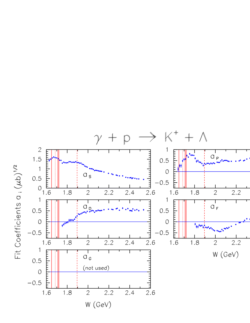
Figure 9: (Color online) Amplitude fit to the differential cross sections for $\gamma+p\rightarrow K^{+}+\Lambda$. The coefficients are defined in Eq. 3. The solid vertical lines mark the well-known $N^{*}$ resonances $S_{11}(1650)$, $P_{11}(1710)$, and $P_{13}(1720)$. The dotted line marks the $\Sigma^{0}$ threshold, and the dashed line marks the $D_{13}(1895)$ position.

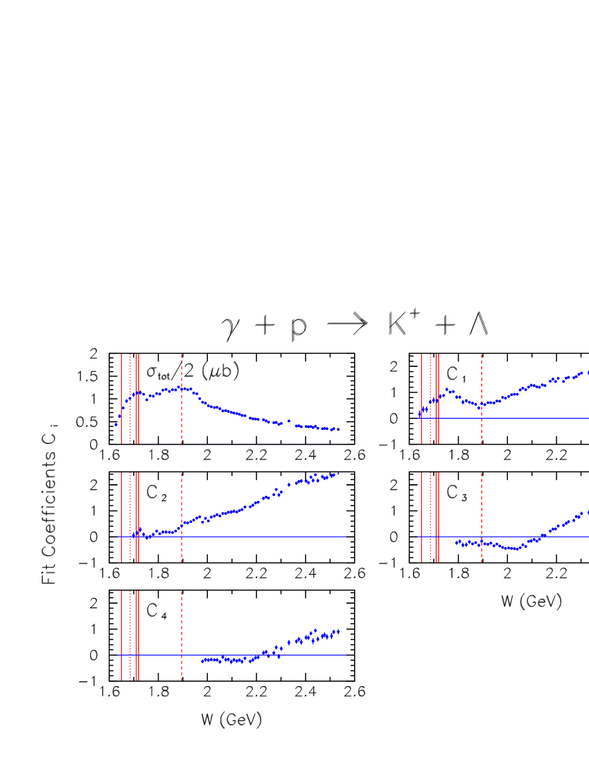
Figure 10: (Color online) Fit to the magnitude of the differential cross sections for $\gamma+p\rightarrow K^{+}+\Lambda$. The coefficients are defined in Eq. 4. The solid vertical lines mark the well-known $N^{*}$ resonances $S_{11}(1650)$, $P_{11}(1710)$, and $P_{13}(1720)$. The dotted line marks the $\Sigma^{0}$ threshold, and the dashed line marks the $D_{13}(1895)$ position.

The differential cross sections for the $\Lambda$ can be compared to the angular distributions for $\Sigma^{0}$ production shown in Fig. 11. The bins in $W$ are the same as before, allowing direct comparison of the panels in Figs. 8 and 11. Results for both hyperons were extracted together, using identical procedures discussed previously. There are 1,280 data points in the $K^{+}\Sigma^{0}$ angular distributions.

Besides the higher reaction threshold, the most significant qualitative difference is that the $\Sigma^{0}$ cross section is not forward peaked in the energy range below 2 GeV. At $W=1.85$ GeV, for example, the cross section peaks near $\cos(\theta_{K^{+}}^{c.m.})=0.35$, or $70^{\circ}$ in the center-of-mass frame. This is consistent with a reaction mechanism for $\Sigma^{0}$ production that is less influenced by $t$-channel exchanges and is more $s$-channel resonance dominated than $\Lambda$ production. The back-angle cross section is less prominent than for the $\Lambda$ case in this energy range as well. Above the nucleon resonance region (above about 2.4 GeV), however, the two channels look quite similar, with characteristic $t$-channel forward peaking.

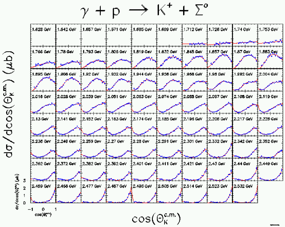
Figure 11: Differential cross sections for $\gamma+p\rightarrow K^{+}+\Sigma^{0}$. The number in each panel designates $W$ ($=\sqrt{s}$). The solid lines are results of the amplitude fits (Eq. 3) discussed in the text.

The coefficients of the amplitude-level fit in Eq. 3 for the $\Sigma^{0}$ angular distributions are shown in Fig. 12. Comparing the $\Lambda$ to the $\Sigma^{0}$ shows that in the $\Sigma^{0}$ case the $D$ wave amplitude plays a more important role, falling and rising with a centroid near 1.85 GeV. The $P$ wave shows no strong bump in the $\Sigma^{0}$, unlike the $\Lambda$. In this case, the $G$ wave coefficient is statistically significant but shows little structure. For completeness, we also show the magnitude-level fit according to Eq. 4 in Fig. 13. The coefficient $C_{1}$ shows some structure, again due to $S-P$ or higher-wave interference. The coefficient $C_{2}$ clearly falls and rises, which can be due to $P$ wave activity or interferences between $S$ and $D$ waves, for example.

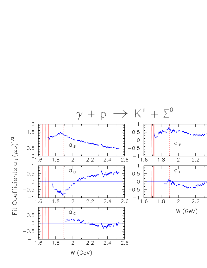
Figure 12: (Color online) Amplitude fit to the differential cross sections for $\gamma+p\rightarrow K^{+}+\Sigma^{0}$. The coefficients are defined in Eq. 3. The solid vertical lines mark the well-known $N^{*}$ resonances $S_{11}(1650)$, $P_{11}(1710)$, and $P_{13}(1720)$. The dotted line marks the $\Sigma^{0}$ threshold, and the dashed line marks the $D_{13}(1895)$ position.

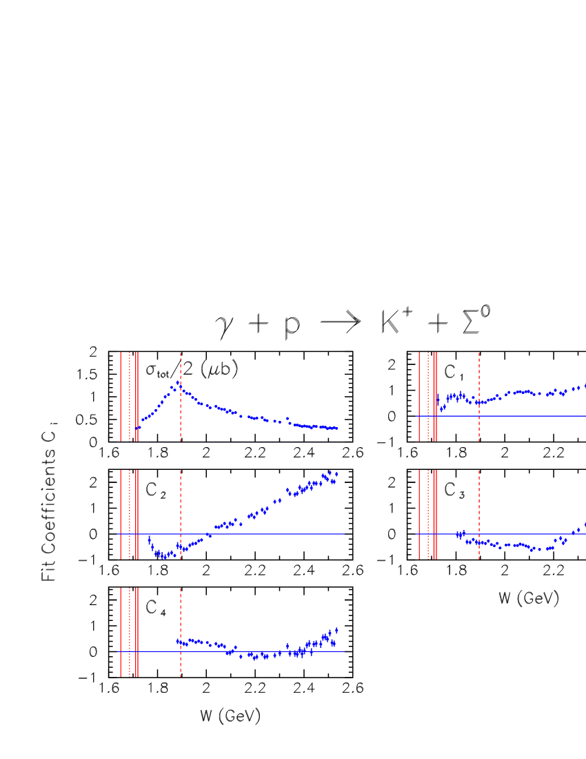
Figure 13: (Color online) Fit to the magnitude of the differential cross sections for $\gamma+p\rightarrow K^{+}+\Sigma^{0}$. The coefficients are defined in Eq. 4. The solid vertical lines mark the well-known $N^{*}$ resonances $S_{11}(1650)$, $P_{11}(1710)$, and $P_{13}(1720)$. The dotted line marks the $\Sigma^{0}$ threshold, and the dashed line marks the $D_{13}(1895)$ position.

Figures 14 and 15 show selected differential cross sections from this experiment compared to previous data and with three published model calculations. The selected panels show about 1/6 of our data, in increments of $\Delta W\approx 80$ MeV to show the trends in the cross sections and the calculations; the exact $W$ values were chosen to emphasize available comparison data.

The results for the angular distributions of photoproduction of $\Sigma^{0}$ are shown in Figs. 16 and  17. Again, the panels are selected to increase in steps of about 80 MeV in $W$, also to allow comparison to previous data.

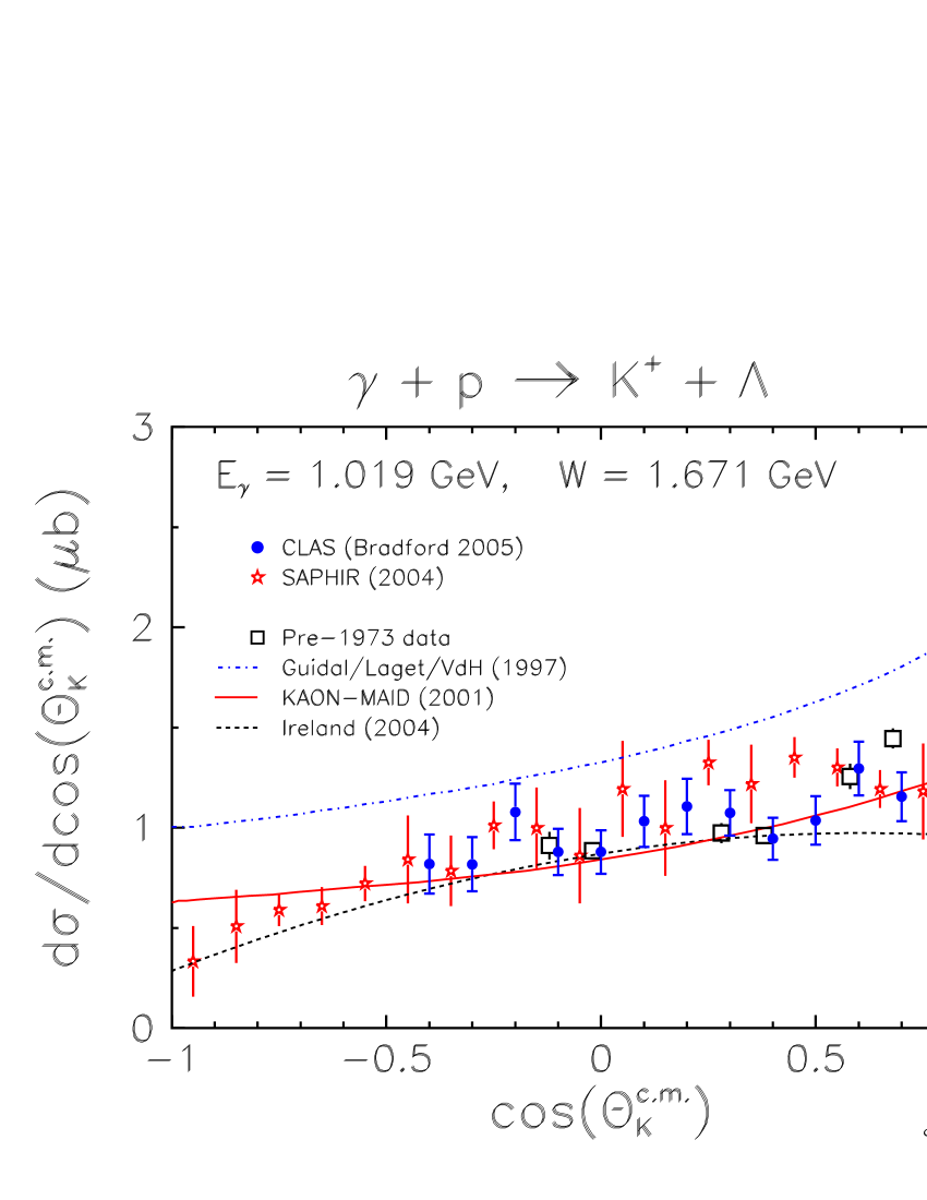
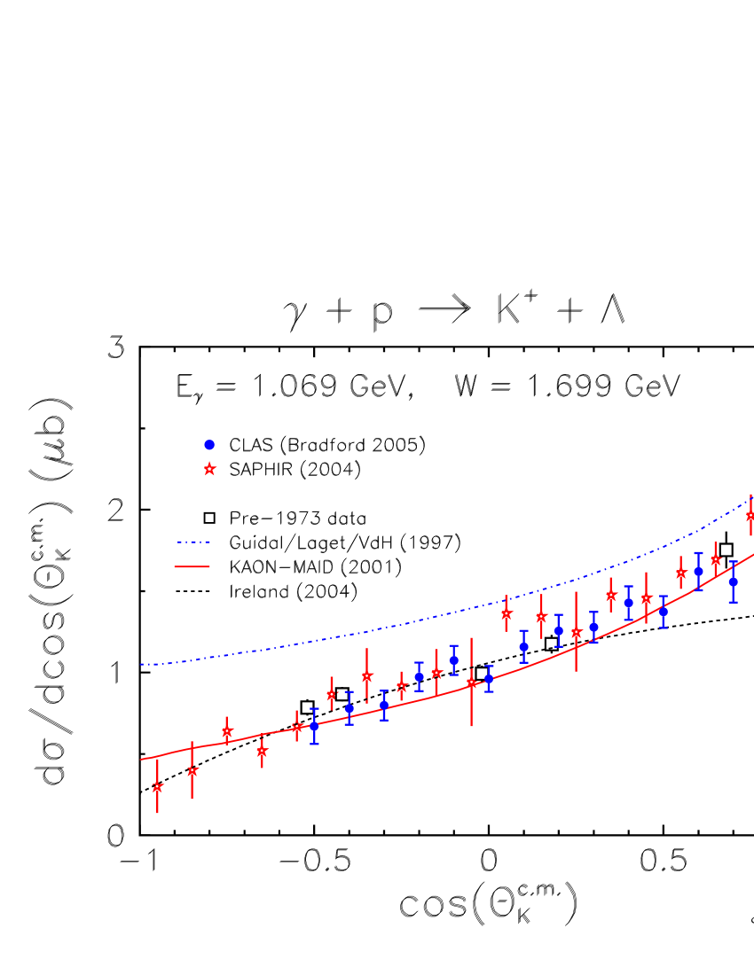
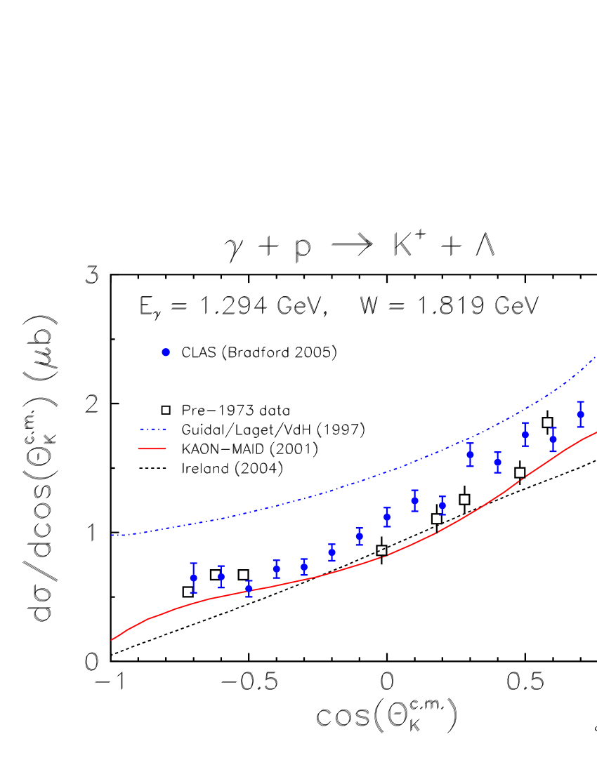
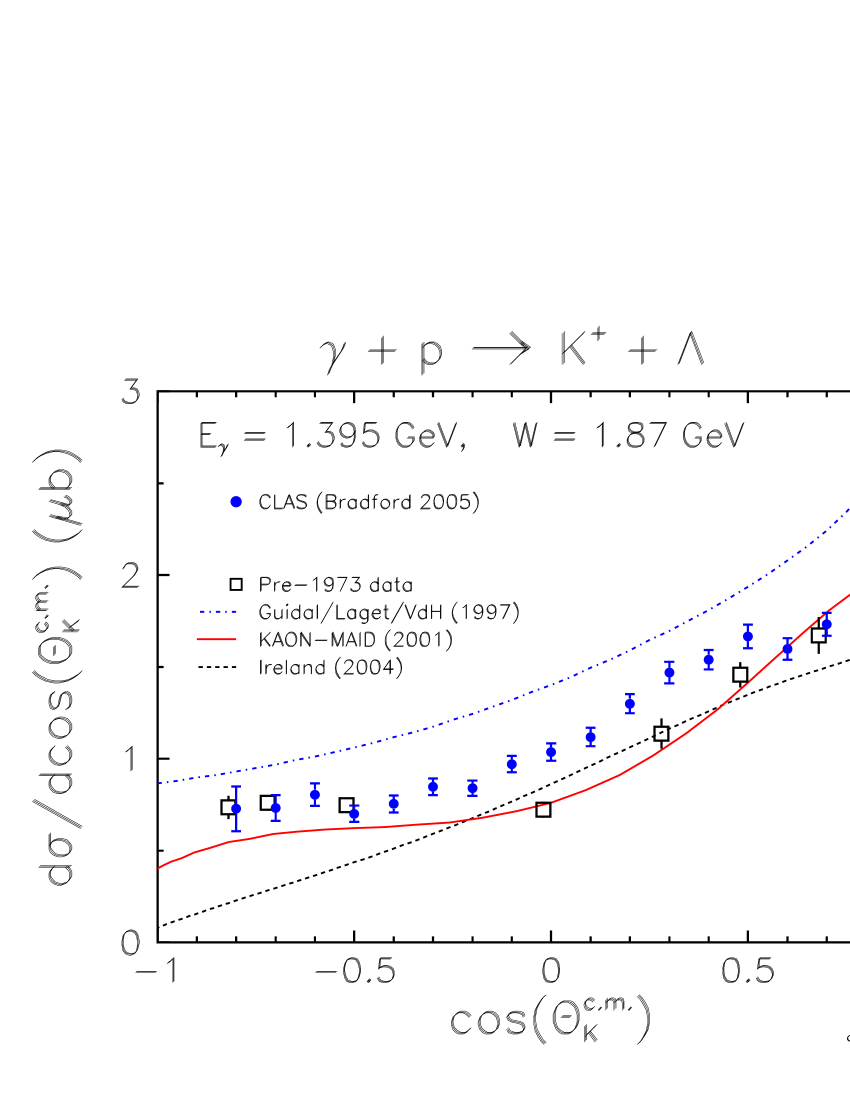
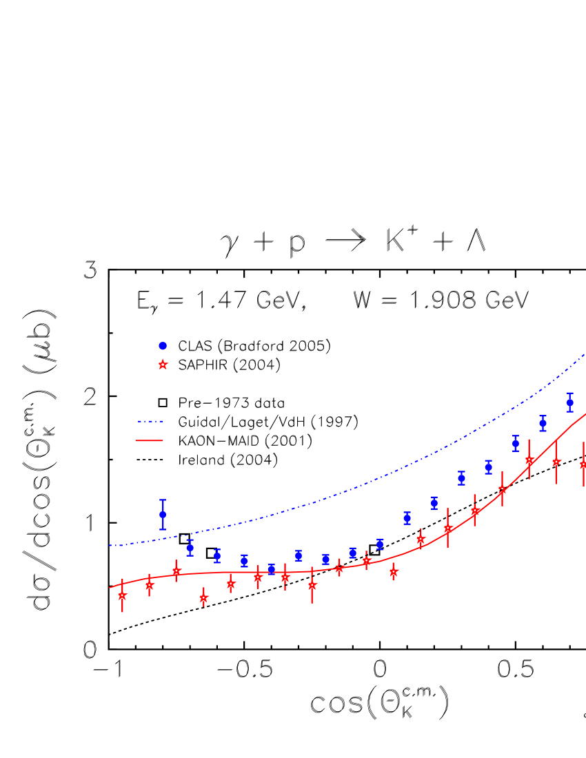
Figure 14: (Color online) Angular distributions for $\gamma+p\rightarrow K^{+}+\Lambda$ for selected bins of total energy $W$. The present CLAS results (blue circles) are shown with statistical and yield-fit uncertainties. Data from SAPHIR bonn2 (open red stars) and from older experiments land (black squares) are also shown. The curves are for effective Lagrangian calculations computed by Kaon-MAID maid (solid red) and Ireland et al. ireland (dashed black), and a Regge-model calculation of Guidal et al. lag1 ; lag2 (dot-dashed blue).

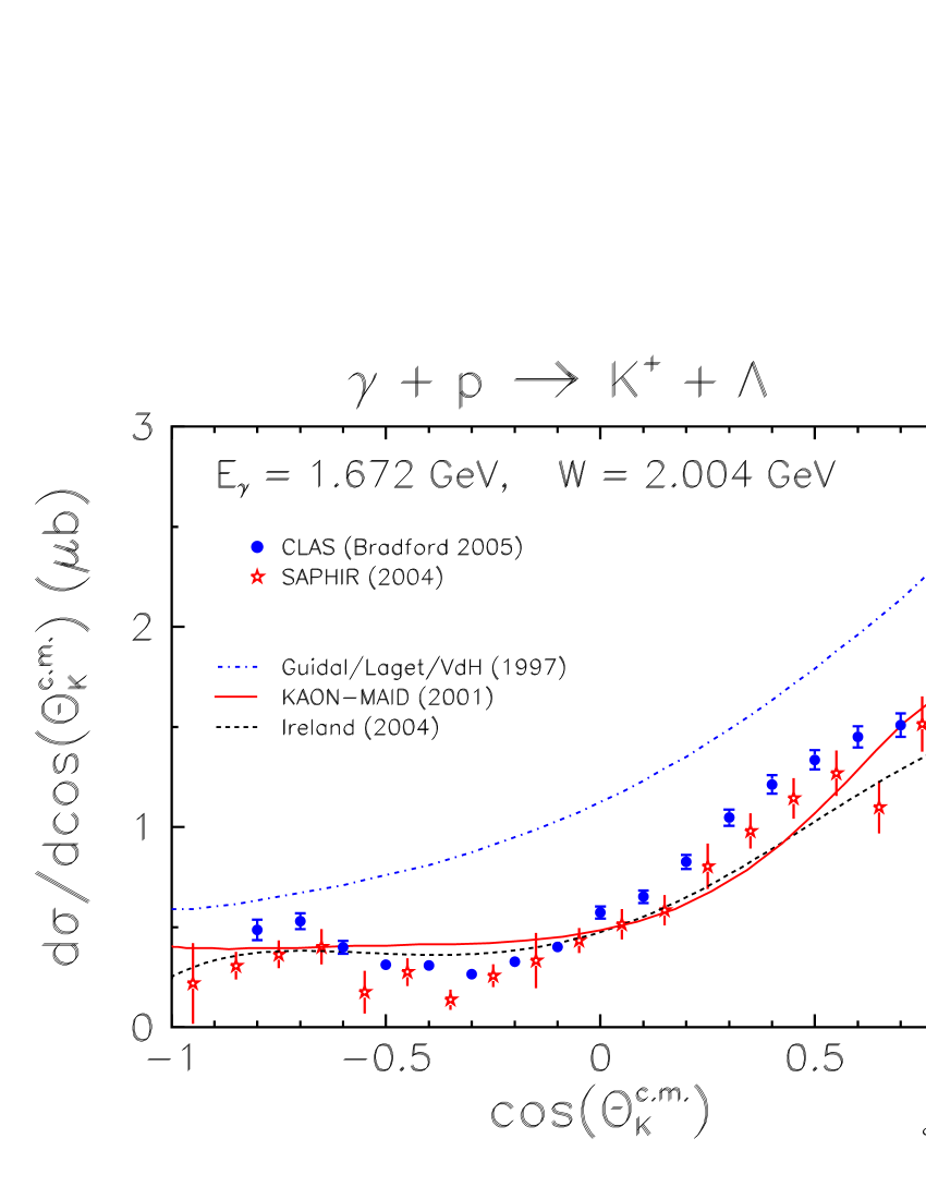
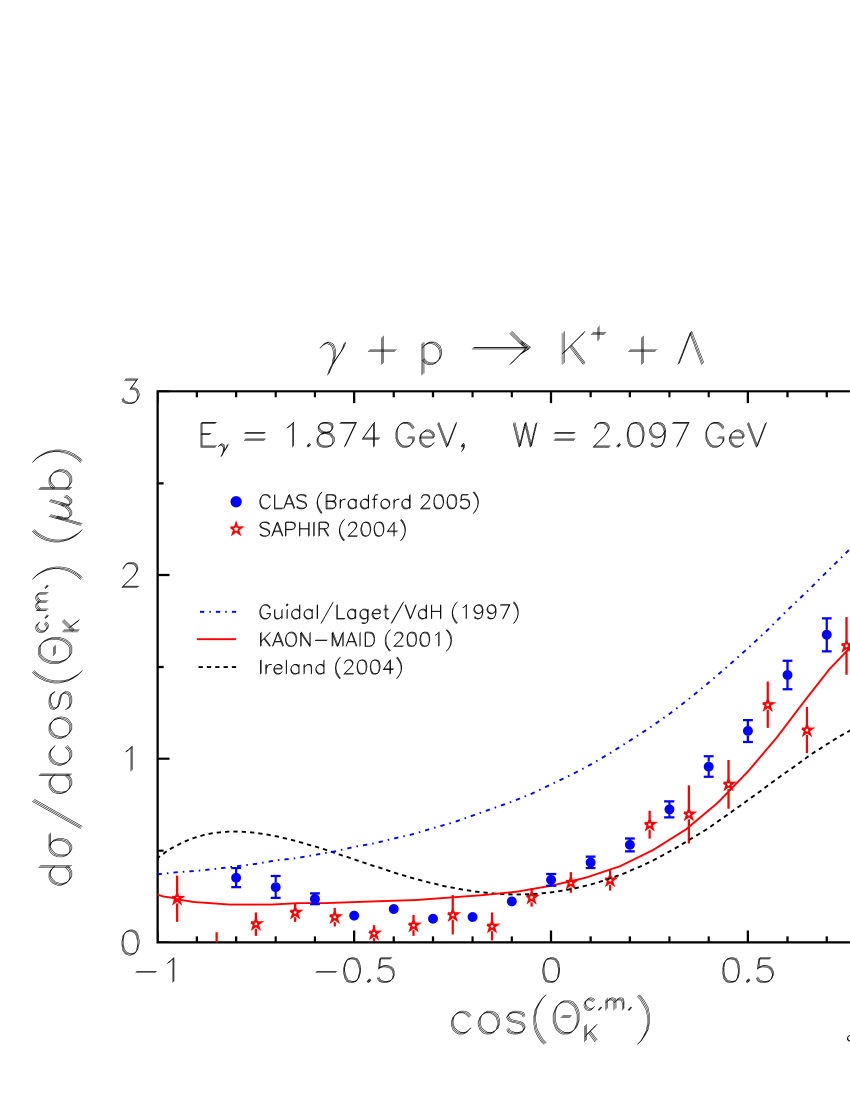
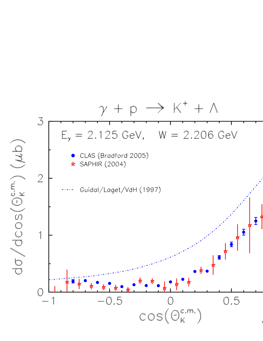
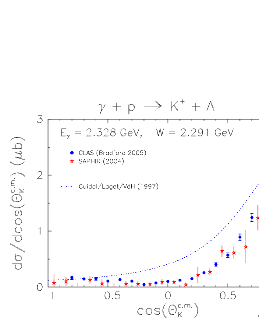
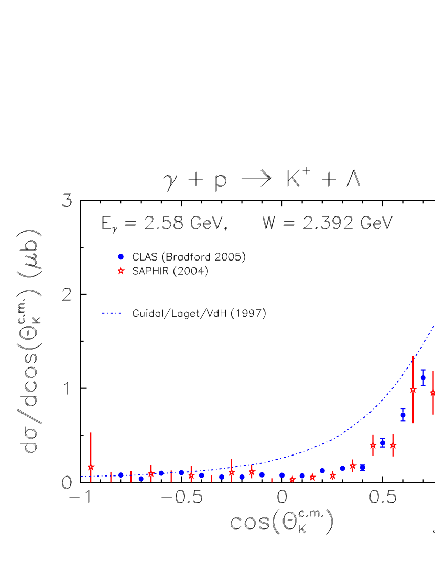
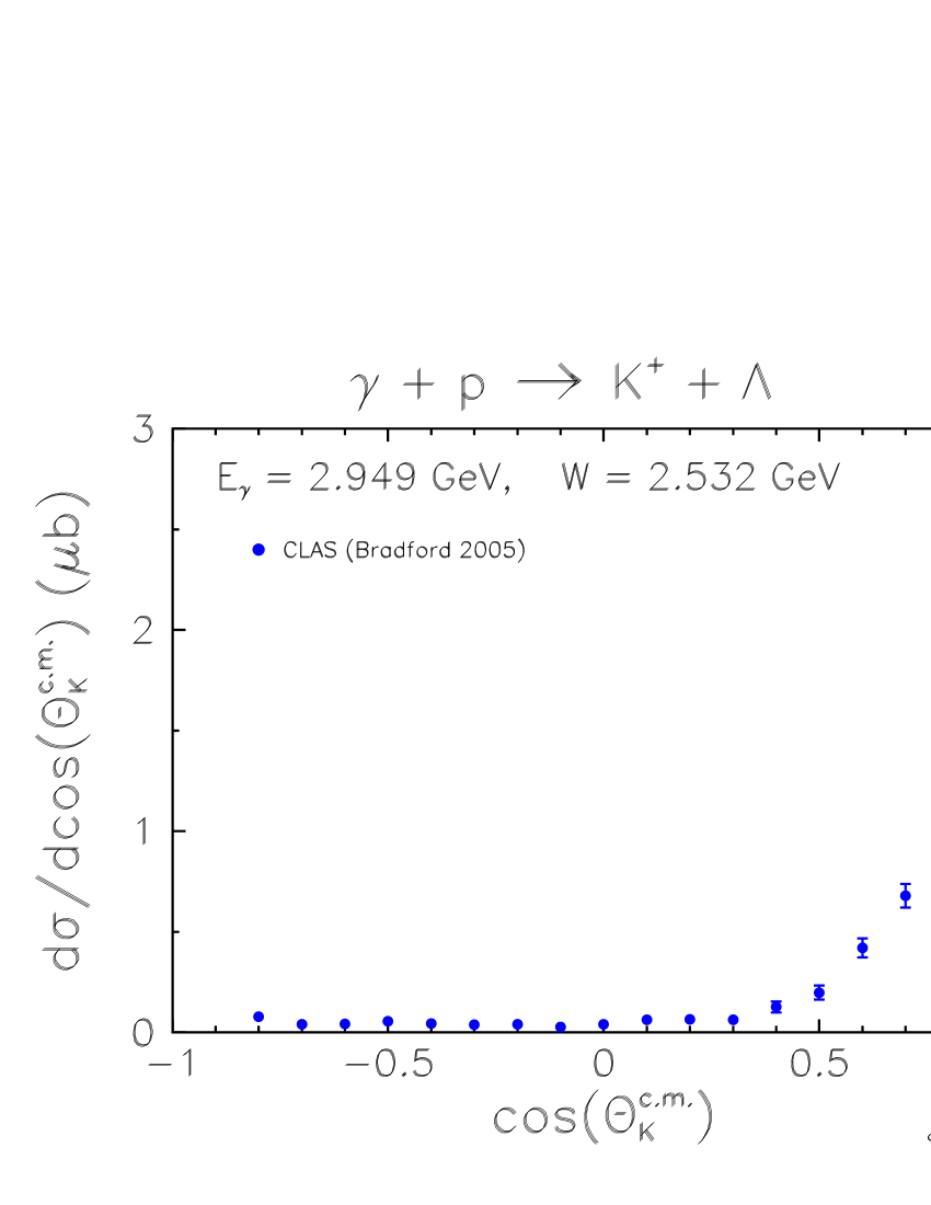
Figure 15: (Color online) Angular distributions for $\gamma+p\rightarrow K^{+}+\Lambda$ for selected bins of total energy $W$. The present CLAS results (blue circles) are shown with statistical and yield-fit uncertainties. Data from SAPHIR bonn2 (open stars) and from older experiments land (black squares) are also shown. The curves are for effective Lagrangian calculations computed by Kaon-MAID maid (solid red) and Ireland et al. ireland (dashed black), and a Regge-model calculation of Guidal et al. lag1 ; lag2 (dot-dashed blue).

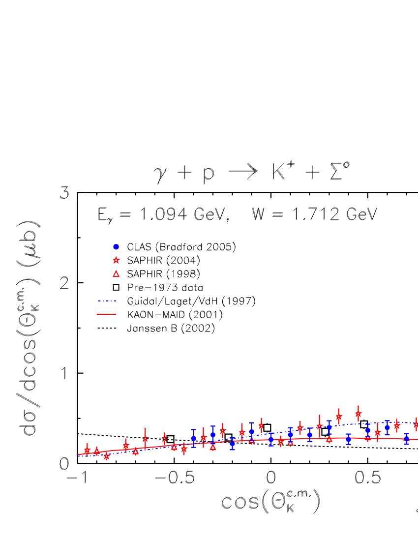
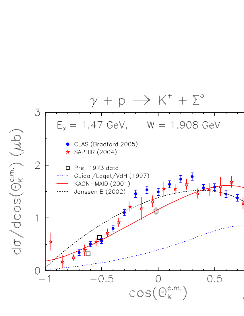
Figure 16: (Color online) Angular distributions for $\gamma+p\rightarrow K^{+}+\Sigma^{0}$ for selected bins of total energy $W$. The present CLAS results (blue circles) are shown with statistical and yield-fit uncertainties. Data from SAPHIR (open stars bonn2 and triangles bonn1 ) and from older experiments land (black squares) are also shown. The curves are for effective Lagrangian calculations computed by Kaon-MAID maid (solid red) and Janssen et al. jan (dashed black), and a Regge-model calculation of Guidal et al. lag1 ; lag2 (dot-dashed blue).

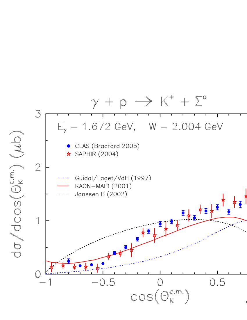
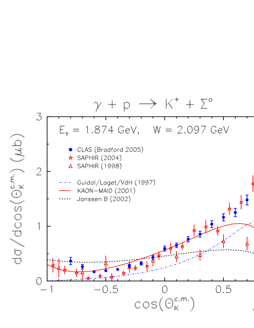
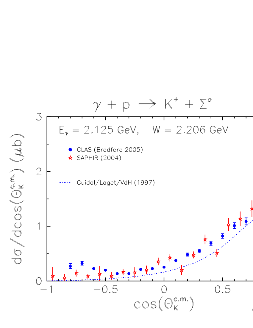
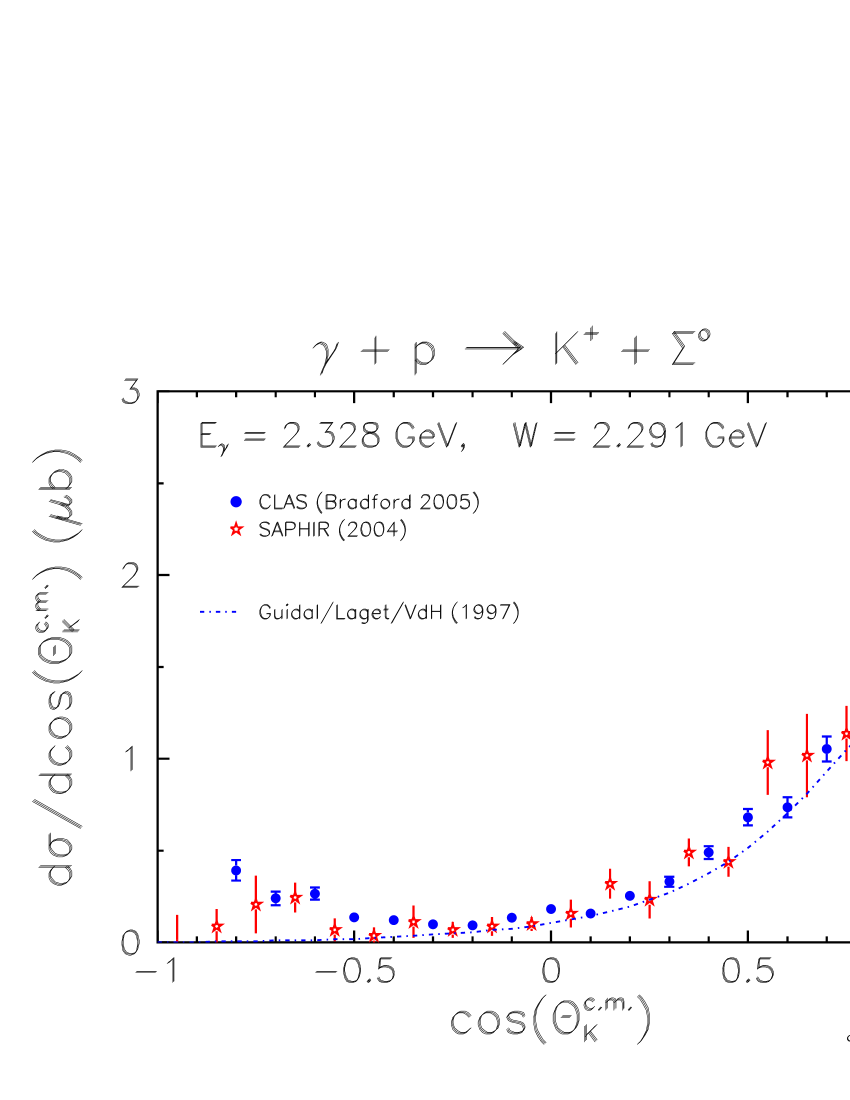
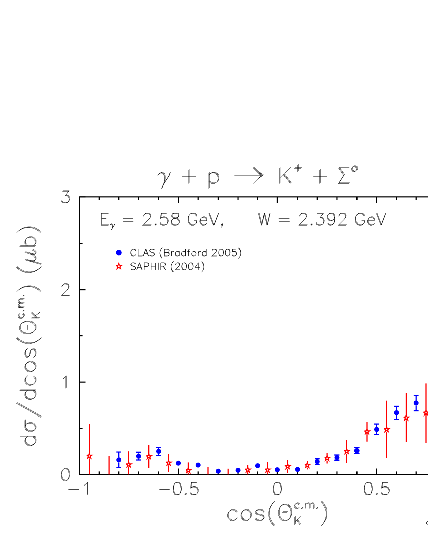
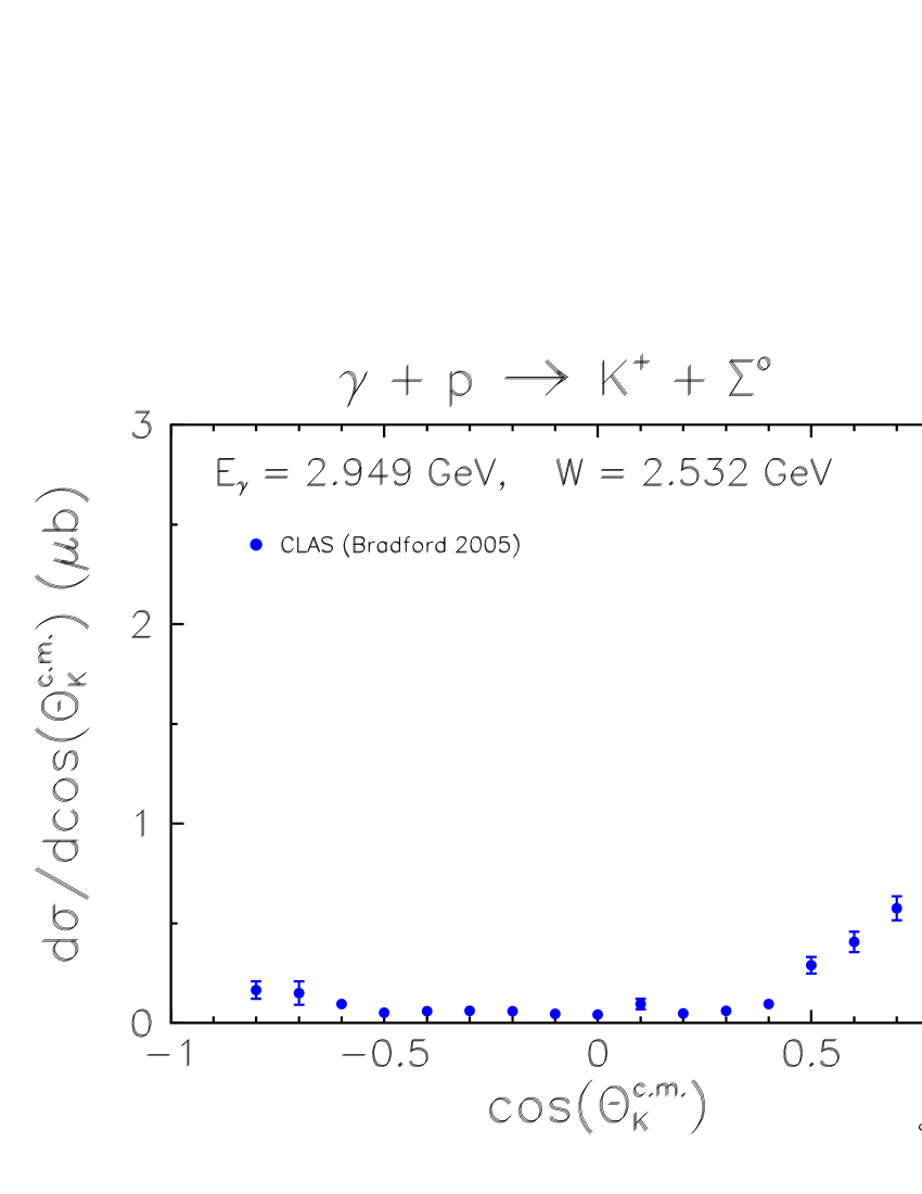
Figure 17: (Color online) Angular distributions for $\gamma+p\rightarrow K^{+}+\Sigma^{0}$ for selected bins of total energy $W$. The present CLAS results (blue circles) are shown with statistical and yield-fit uncertainties. Data from SAPHIR (open stars bonn2 and triangles bonn1 ) and from older experiments land (black squares) are also shown. The curves are for effective Lagrangian calculations computed by Kaon-MAID maid (solid red) and Janssen et al. jan (dashed black), and a Regge-model calculation of Guidal et al. lag1 ; lag2 (dot-dashed blue).

V.2 $W$ Dependence

Resonance structure in the $s$-channel should appear most clearly in the $W$ dependence of the cross sections. In Fig. 18 we show the $K^{+}\Lambda$ cross section at selected angles. The corresponding information for the $K^{+}\Sigma^{0}$ channel is shown in Fig. 19. We discuss these results in the next section.

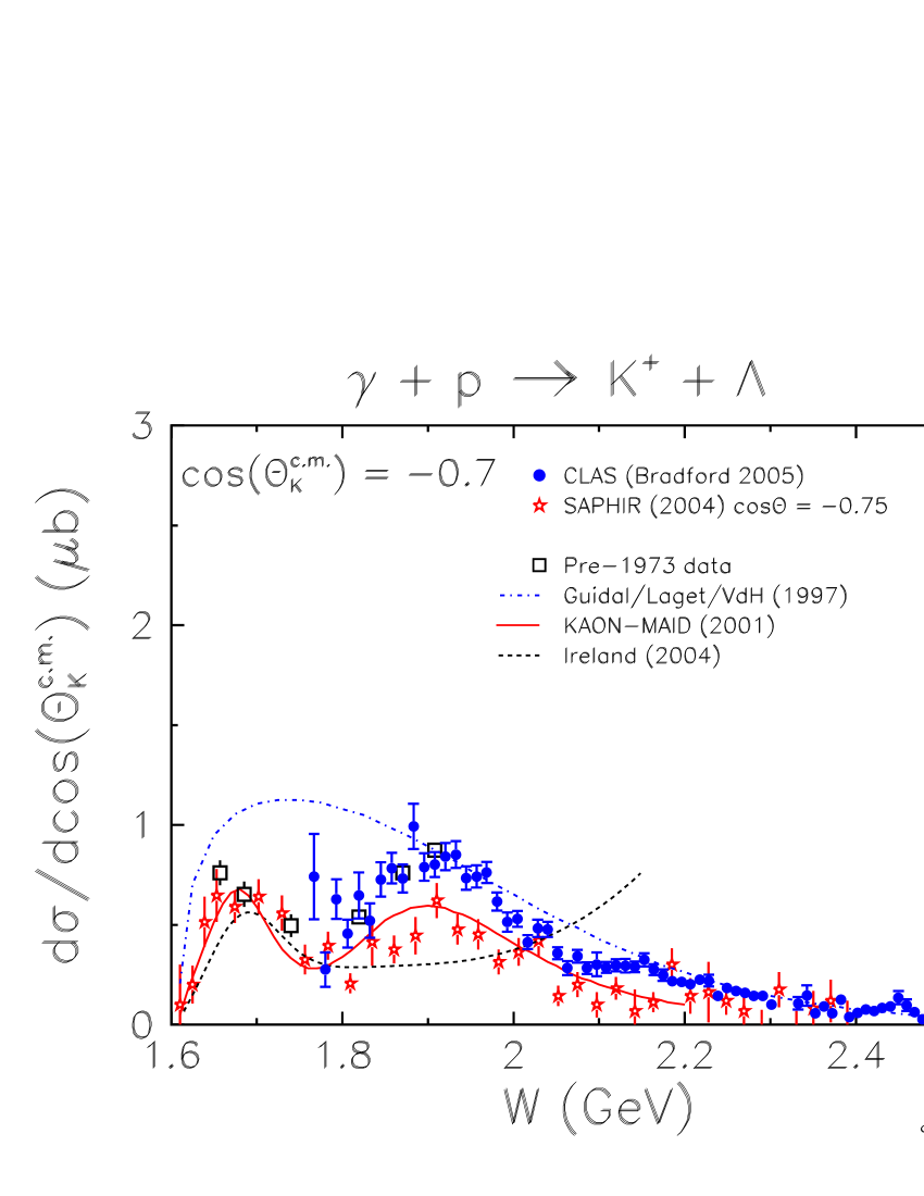
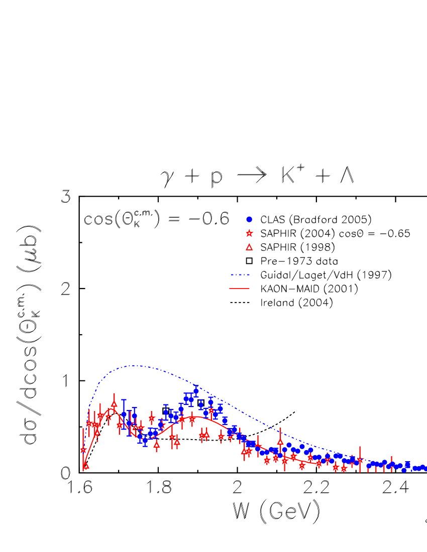
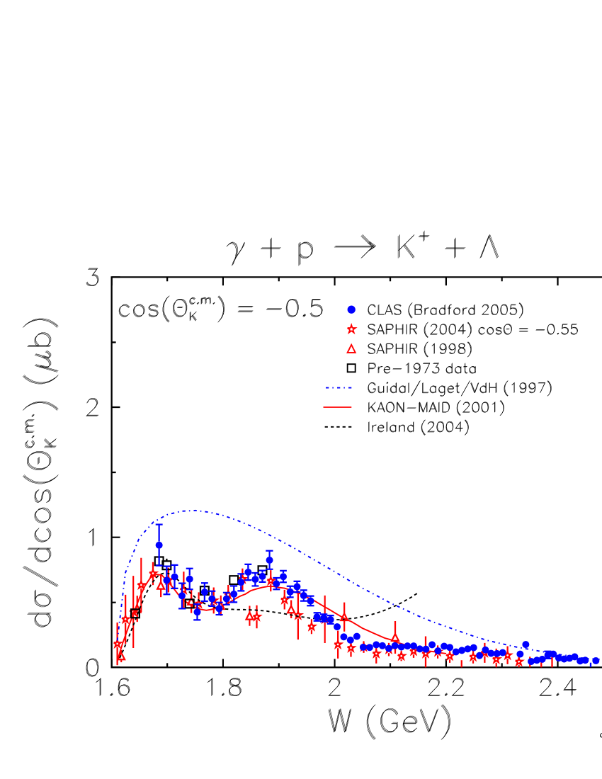
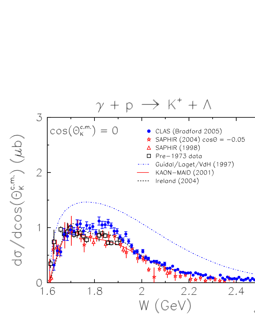
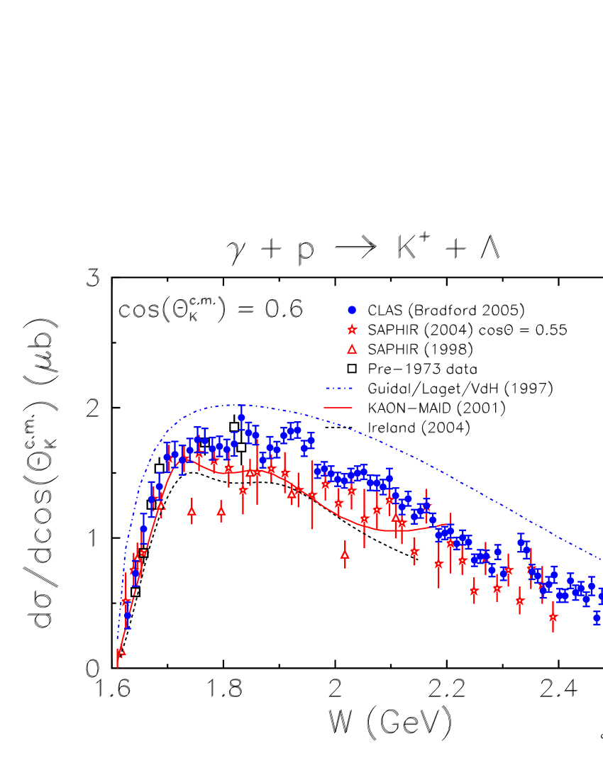
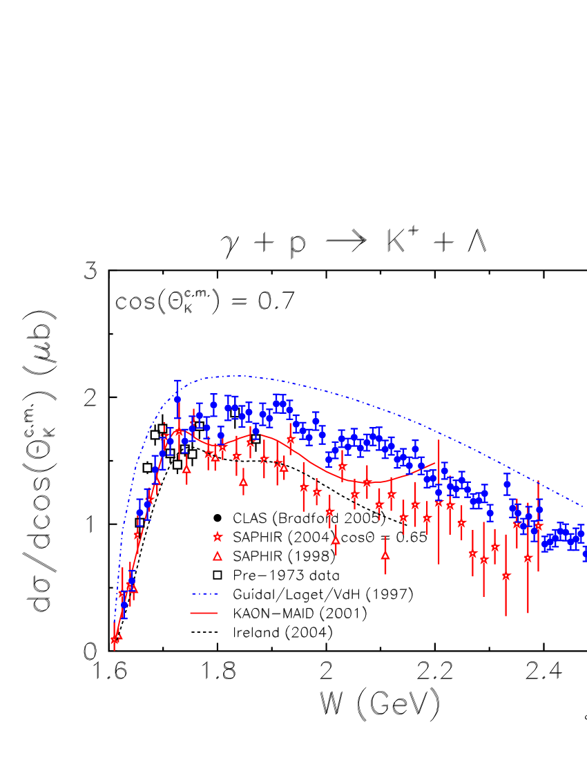
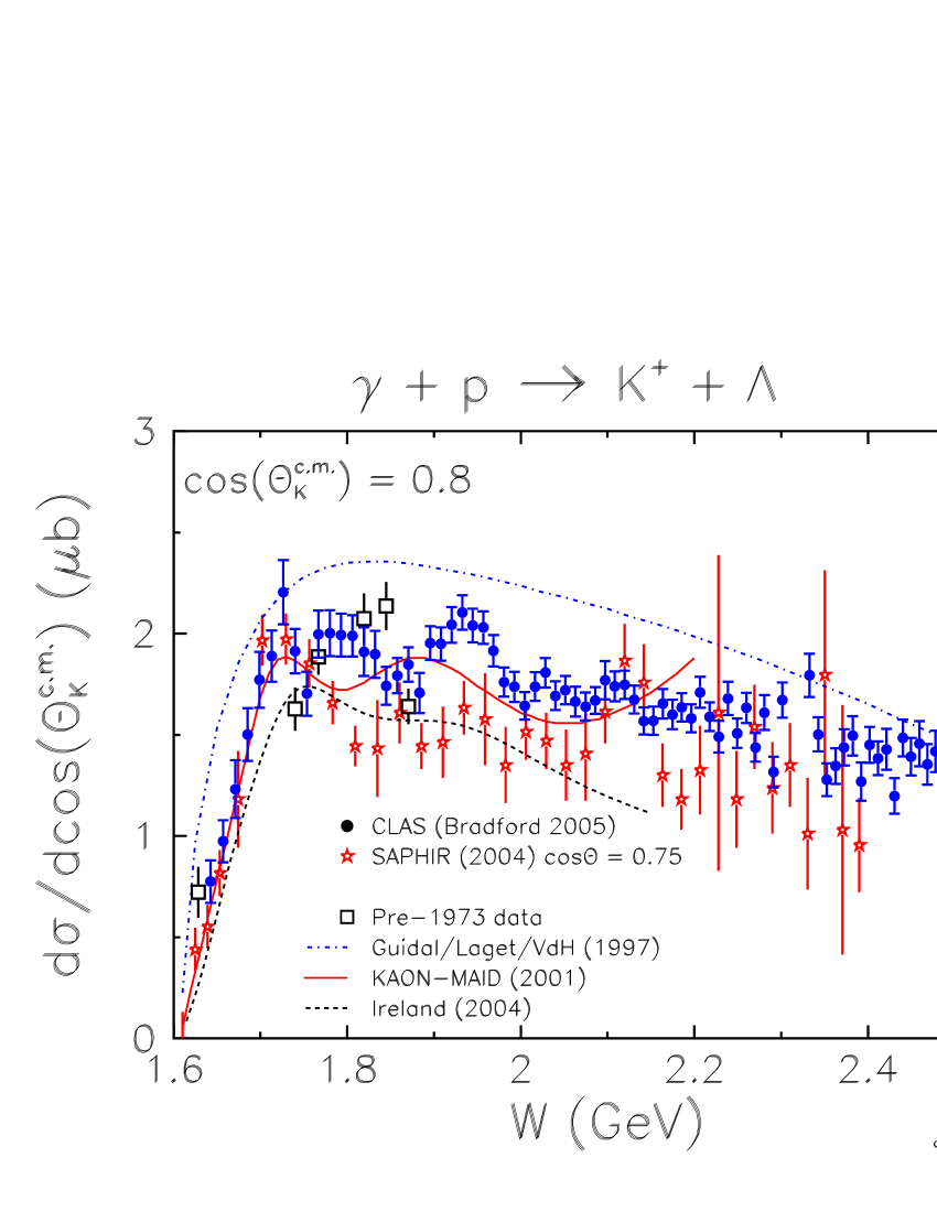
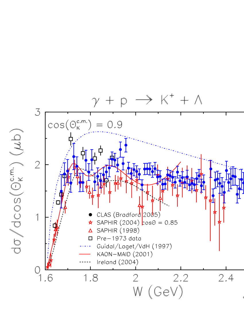
Figure 18: (Color online) Energy distributions for $\gamma+p\rightarrow K^{+}+\Lambda$ for selected c.m. kaon angles. CLAS results (blue circles) are shown with statistical and yield-fit uncertainties. Data from SAPHIR (open stars bonn2 , triangles bonn1 ) and older experiments land (black squares) are also shown. The curves are for effective Lagrangian calculations computed by Kaon-MAID maid (solid red) and Ireland et al. ireland (dashed black), and a Regge-model calculation of Guidal et al. lag1 ; lag2 (dot-dashed blue).

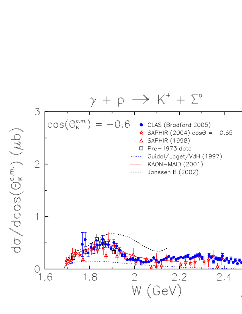
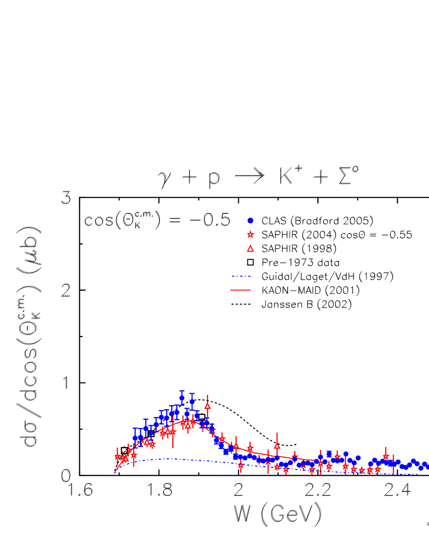
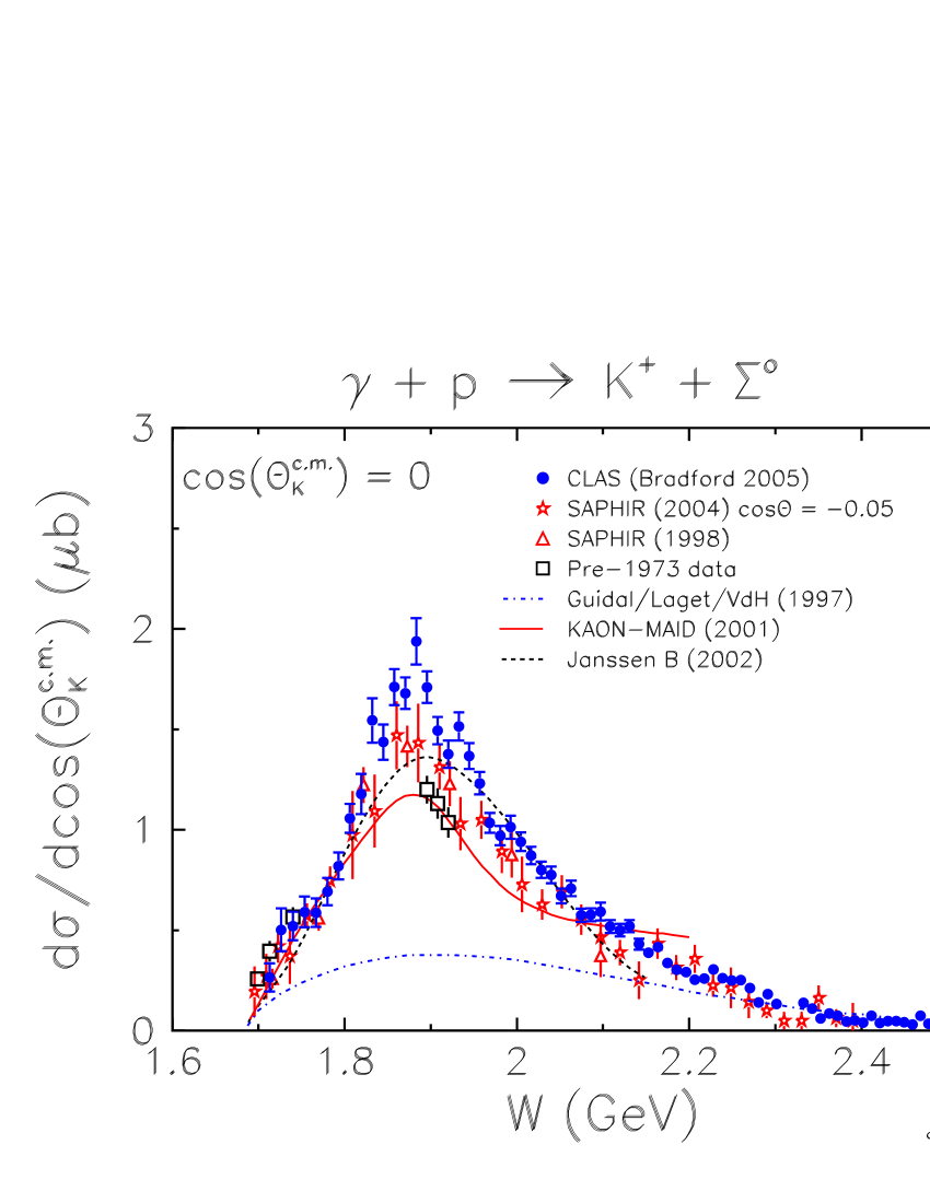
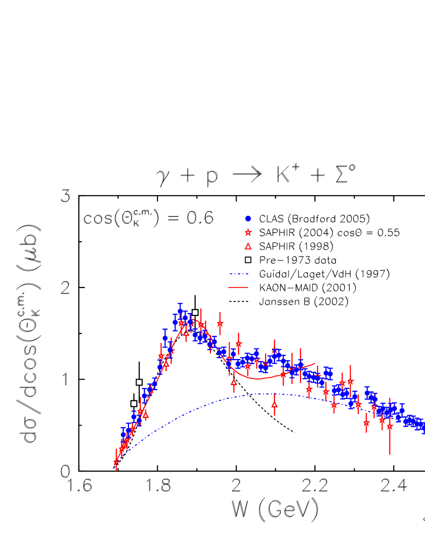
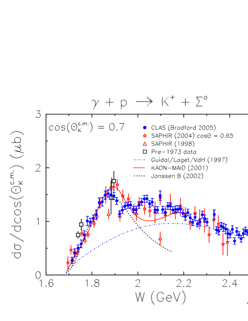
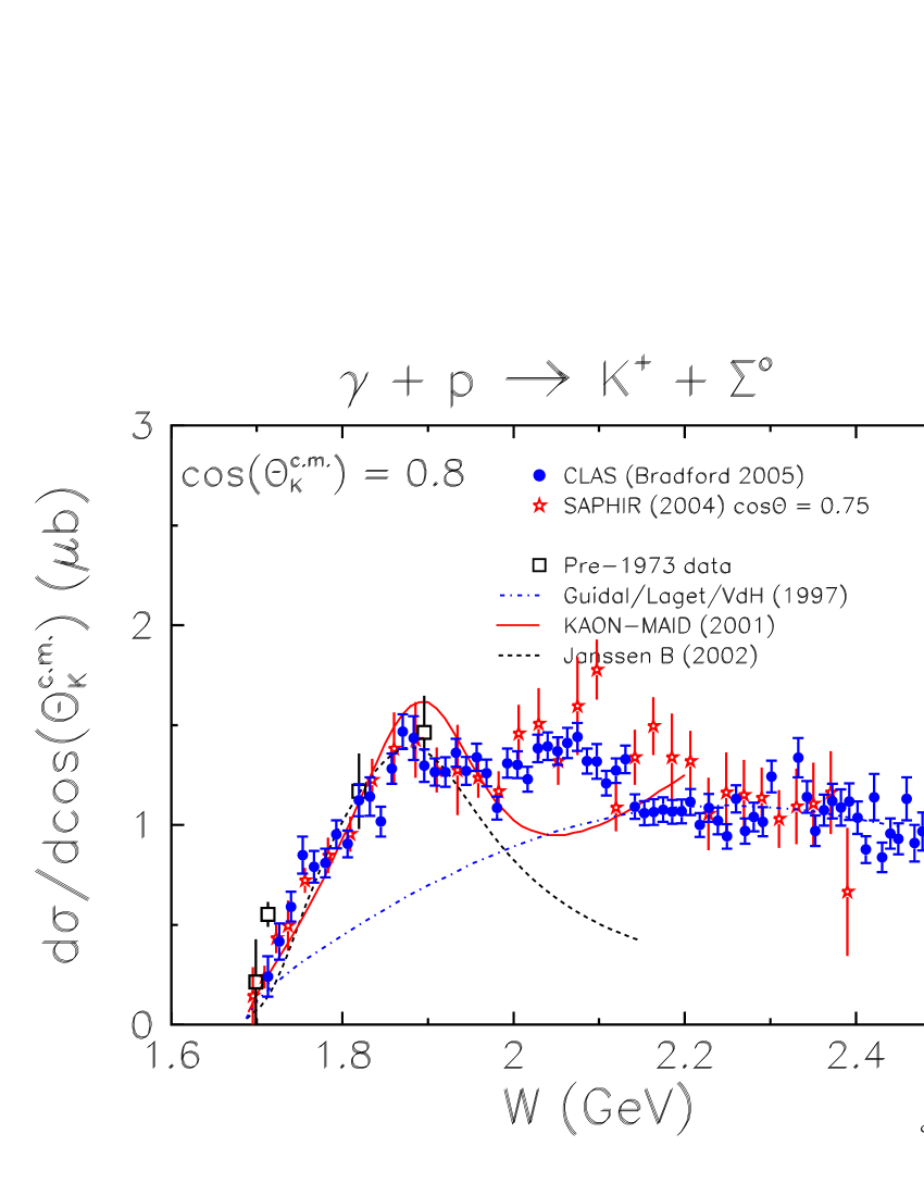
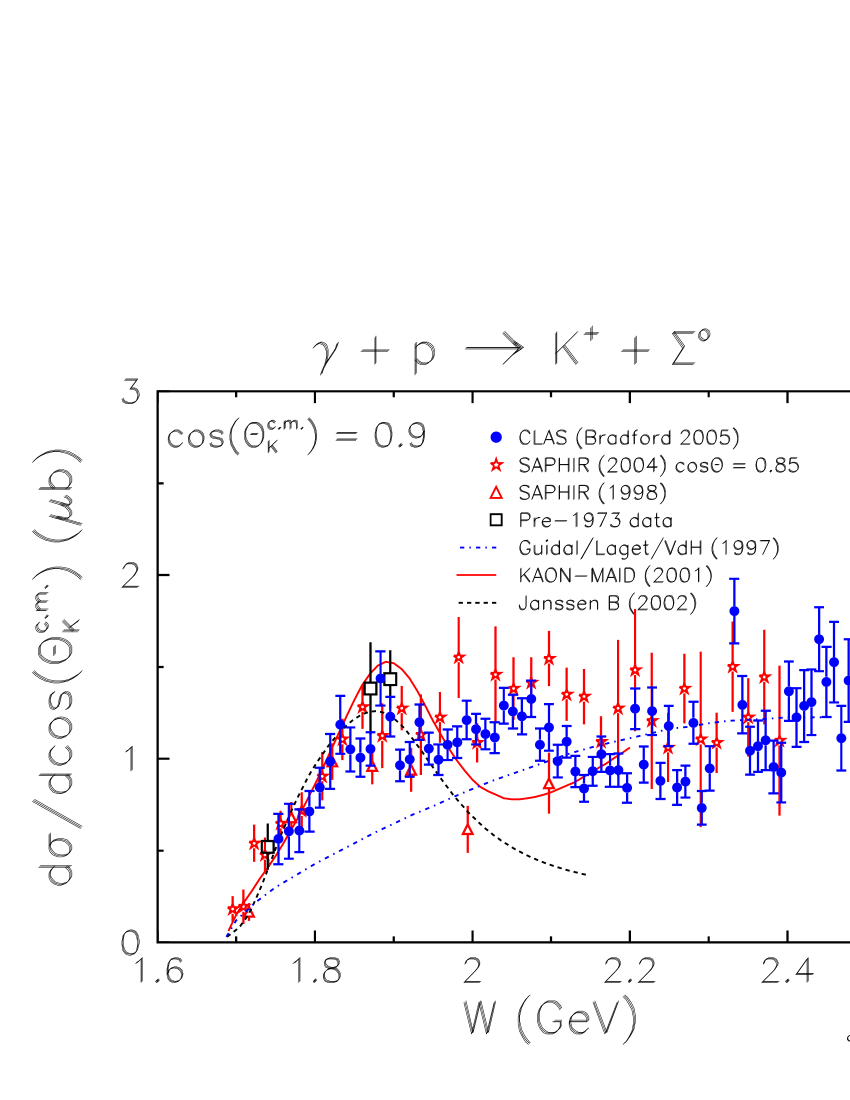
Figure 19: (Color online) Energy distributions for $\gamma+p\rightarrow K^{+}+\Sigma^{0}$ for selected c.m. kaon angles. CLAS results (blue circles) are shown with statistical and yield-fit uncertainties. Data from SAPHIR (open stars bonn2 , triangles bonn1 ) and older experiments land (black squares) are also shown. The curves are for effective Lagrangian calculations computed by Kaon-MAID maid (solid red) and Janssen et al. jan (dashed black), and a Regge-model calculation of Guidal et al. lag1 ; lag2 (dot-dashed blue).

The full set of numerical results from this experiment are available from various archival sources, including a Ph.D. thesis bradford , the CLAS online database clasdb , or private communication contact .

VI DISCUSSION

VI.1 Comparison to Previous Data

Figures 14, 15, 16, and 17 show a sample of the differential cross section for $\Lambda$ and $\Sigma^{0}$ hyperon photoproduction as a function of angle for a set of $W$ values. For comparison, we can examine the previous large-acceptance experiment from SAPHIR at Bonn bonn1 ; bonn2 . There is also a set of measurements that was accumulated from the late 1950’s to the early 1970’s using small-aperture magnetic spectrometers at CalTech brody ; peck ; groom ; donoho , Cornell anderson ; thom , Bonn bleckman ; feller , Orsay decamp , DESY going , and Tokyo fujii . These results are compiled, for example, in Ref land .

The agreement with data from SAPHIR is fair or good, but there are some discrepancies. The CLAS results are generally more precise, having statistical uncertainties that are about 1/4 as large, with about twice as many energy bins. The SAPHIR experiment had better backward-angular coverage at low energies as well as coverage at extreme forward angles where CLAS has an acceptance hole. The measurements agree within the estimated uncertainties at some angles and generally near threshold energies, but CLAS measures consistently larger $K^{+}\Lambda$ cross sections at most kaon angles and for $W>1.75$ GeV. This is discussed in more detail below in the context of the total cross sections, where it appears that there is an energy-independent scale factor of about 3/4 in going from the CLAS to the SAPHIR $K^{+}\Lambda$ results. The data for the $K^{+}\Sigma^{0}$ channel are generally in better agreement overall: the two experiments agree within their stated systematic uncertainties.

We collected the historic (pre-1973) results from different measurements and plotted them together. The error bars are taken as the quoted random uncertainties, with no consideration of the quoted systematic uncertainties. While these early experiments did not span the large $W$ and angular range of the recent experiments, they did make high-precision measurements at selected kinematics. There are 144 $K^{+}\Lambda$ points and 57 $K^{+}\Sigma^{0}$ points that, overall, are in fair agreement with the CLAS results. At backward angles the historic data are in very good agreement with the present results from CLAS; at forward angles the agreement is fair or good. In the mid-range of angles, the historic results are lower than our results, and more similar to the SAPHIR data.

The fit coefficients presented in Figs. 9 and 12 are in good qualitative agreement with results published by SAPHIR, apart from an arbitrary overall change in sign. The CLAS results generally have finer binning and smaller estimated uncertainties away from threshold. However, our vertical scales do not agree with SAPHIR, though it is clear their units are incorrect as given, since they should be $\sqrt{\mu b}$.

Total cross sections, $\sigma_{tot}$, for $\gamma+p\rightarrow K^{+}+\Lambda$ and $\gamma+p\rightarrow K^{+}+\Sigma^{0}$ can be calculated from the integrated angular distributions. There is some danger in the integration procedure since (i) it requires some model of the reactions which may bias the resulting fit, and (ii) in the absence of complete angular coverage there is also the problem of extrapolating the fit into the unmeasured section of phase space. Our procedure for extracting and calculating the total cross sections was based on fitting $d\sigma/d\cos(\theta_{K^{+}}^{c.m.})$ in two ways: using Eq. 4 to fit the magnitude directly, and Eq. 3 to fit the partial wave amplitudes. In the magnitude fit, one of the coefficients directly gives $\sigma_{tot}$ and its associated error. In the amplitude fit $\sigma_{tot}$ is easily computed from the set of fit parameters, but the error is difficult to extract since the fit parameters and their errors are correlated. We estimated the systematic bias in our integrations by taking the standard deviation of the two resultant values as an additional uncertainty, and this was added in quadrature to the other estimated uncertainties.

The total cross section results are shown in Figs. 20 and  21. The error bars combine statistical and estimated systematic uncertainty due to the fitting procedure. The gaps in the spectra at $W=2.375$ and $2.400$ GeV stem from photon tagger failures at those energies. For comparison we show two previously published data sets from Bonn bonn1 ; bonn2  bonnnote . Also, bubble chamber data for the total cross sections came from Erbe et al. (ABBHHM) erbe . Also shown are model curves for two calculations, the effective Lagrangian model embodied in Kaon-MAID maid and the Regge model of Guidal, Laget, and Vanderhaeghen lag1 ; lag2 . The CLAS results for $\sigma_{tot}$ differ from the Bonn results in an unexpected way, namely that the Bonn $K^{+}\Lambda$ cross section is smaller than the CLAS result by a factor of close to $3/4$. This is in contrast to the $K^{+}\Sigma^{0}$ results, where the CLAS and the Bonn results are in good agreement: the values of $\sigma_{tot}$ agree well within their quoted systematic uncertainties. We note that the CLAS results for the two hyperons used exactly the same photon normalizations, and that the hyperon yield extractions for both cases were made together, as discussed above. The acceptance calculations for the CLAS results used the same software as well, differing only in the input events used for the calculations. In short, we have not found any reason within the CLAS analysis for one channel agreeing well with previous work and the other not. Both results are consistent with the ABBHHM data erbe .

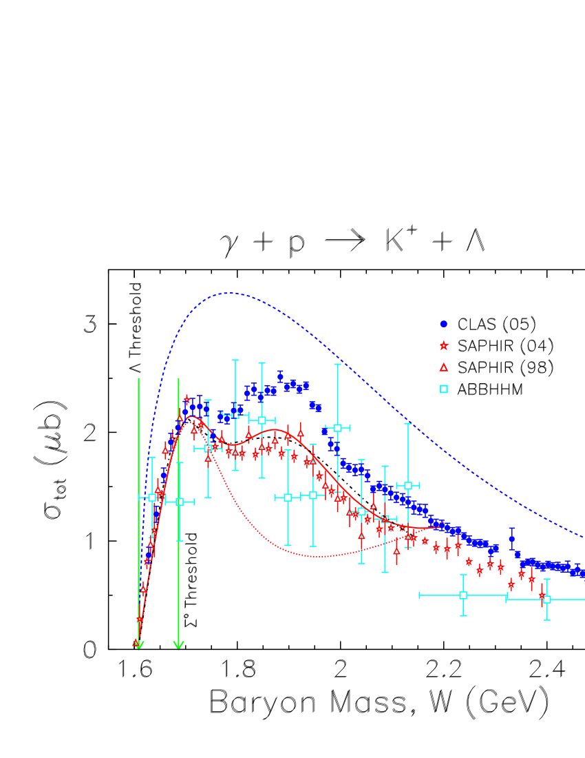
Figure 20: (Color online) Total cross section for $\gamma+p\rightarrow K^{+}+\Lambda$. The data from CLAS (blue circles) are shown with combined statistical and fitting uncertainties. Also shown are results from two publications from SAPHIR (red stars (2004) bonn2 , red triangles (1998) bonn1 ), and the ABBHHM Collaboration (light blue squares) erbe . The curves are from a Regge model (dashed blue) lag1 ; lag2 , Kaon-MAID (solid red) maid , Kaon-MAID with the $D_{13}(1895)$ turned off (dotted red), and Saghai et al. (dot-dashed black) sag .

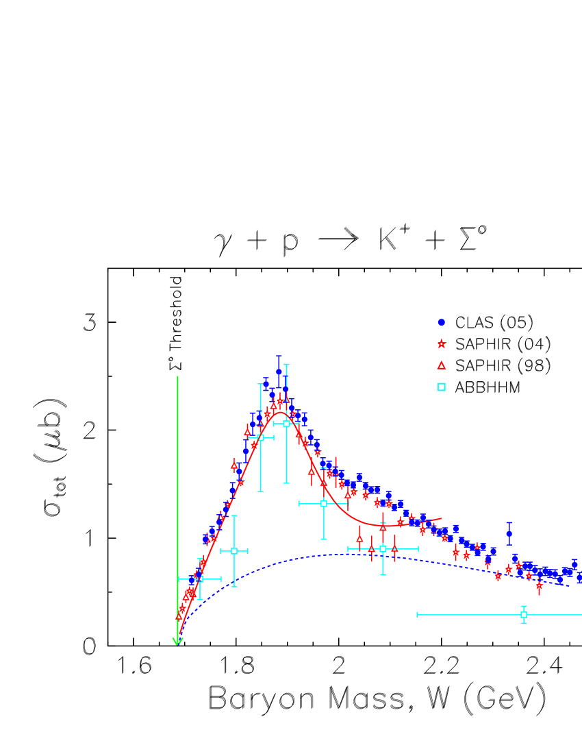
Figure 21: (Color online) Total cross section for $\gamma+p\rightarrow K^{+}+\Sigma^{0}$. The data are from CLAS (blue circles) are shown with combined statistical and fitting uncertainties, Also shown are results from two publications from SAPHIR (red stars (2004) bonn2 , red triangles (1998) bonn1 ), and the ABBHHM Collaboration (light blue squares) erbe . The curves are from a Regge model (dashed blue) lag1 ; lag2 and Kaon-MAID (solid red) maid .

The CLAS $\sigma_{tot}$ results for $K^{+}\Lambda$ show a prominent peak centered near 1.9 GeV. It does not resemble a simple single Lorentzian, reflective of the expectation that several resonant structures are present in this mass range. The peak near 1.7 GeV is consistent with contributions from the $P_{11}(1710)$ and $P_{13}(1720)$. In the case of $K^{+}\Sigma^{0}$, the $\sigma_{tot}$ curve shows the previously seen strong peak centered at 1.88 GeV, and in addition there is a slight shoulder at about 2.05 GeV. The location of the strong peak is consistent with the mass of several well-established $\Delta$ resonances which may contribute to an isospin 3/2 final state.

VI.2 Comparison to Reaction Models

The model calculations shown in this paper were not fitted to the present results. The effective Lagrangian calculations, in particular, were fitted to the previous data shown in this paper, and have, therefore, at least fair agreement with those earlier results. However, since in the case of $K^{+}\Lambda$ production we have some disagreement with the SAPHIR data in the mid-range of angles, we cannot expect these calculations to be in quantitative agreement with us. It is nevertheless interesting to see what the more copious CLAS results seem to indicate in comparison to a few of these previous models.

The Regge-model calculation lag1 ; lag2 shown in the preceding figures uses only $K$ and $K^{*}$ exchanges, with no $s$-channel resonances. The model was constructed to fit high-energy kaon photoproduction data slac , for $W$ between 5 and 16 GeV, and may be expected to reproduce the average behavior of the cross section in the nucleon resonance region. However, extrapolated down to the resonance region, the model overpredicts the size of the $\Lambda$ cross section and underpredicts that of the $\Sigma^{0}$. This is evident in all the graphs, but is especially easily seen in the total cross sections, Figs. 20 and 21. Since it is a pure $t$-channel reaction model, it cannot produce a rise at back angles as seen for the $\Lambda$, and illustrates the need for $s$- and $u$-channel contributions to understand that feature.

Two hadrodynamic models mart ; jan based on similar effective Lagrangian approaches are also shown. Both emphasize the addition of a small set of $s$-channel resonances to the non-resonant Born terms, and differ in their treatment of hadronic form factors and gauge invariance restoration. As both were fitted to the previous data from SAPHIR bonn2 , they are expected to be in somewhat poorer agreement with our $K^{+}\Lambda$ than our with $K^{+}\Sigma^{0}$ data.

Both models contain a set of known $s$-channel $N^{*}$ resonances: $S_{11}(1650)$, $P_{11}(1710)$, and $P_{13}(1720)$. The model of Mart et al. mart which is used in the Kaon-MAID calculations contains an additional $D_{13}$(1895) resonance in its $K^{+}\Lambda$ description. In the $K^{+}\Lambda$ case, the calculations of Ireland et al. ireland are shown since they represent an update of the earlier work of Janssen et al. jan . These calculations included photon beam asymmetry zegers and electroproduction mohring data points in the dataset used for fitting. The curves displayed on Figs. 14,  15, and 18 contain the set of known resonances plus an additional $P_{11}$(1895) resonance. This combination was found to give the best quantitative agreement with the dataset used for fitting. The analysis of Ref. ireland was restricted to a study of the $K^{+}\Lambda$ channel, so for comparison with the present $K^{+}\Sigma^{0}$ data, we use slightly older calculations jan which contain an additional $D_{13}$(1895).

The CLAS $K^{+}\Lambda$ results, which show a structure that varies in width and position with kaon angle, suggests an interference phenomenon between several resonant states in this mass range, rather than a single, well-separated resonance. This should be expected, since several $N^{*}$ resonances with one- and two-star PDG ratings occupy this mass range. From Fig. 18, the best qualitative modeling of the structure near 1.9 GeV at backward angles is given by Kaon-MAID maid , but the model seems to diverge from the trends of the data at forward angles. The calculation of Ref. ireland gives a poor description of the data in the 1.9 GeV region at backward angles, but at forward angles it is similar to the Kaon-MAID calculation. Using the model curves as a guide, we see that a fixed position for a single isolated resonance near 1.9 GeV is not consistent with the small ($\sim 50$ MeV) variation with angle of the feature seen in the cross sections.

In the $\Sigma^{0}$ case there is some indication of a structure above the large peak at 1.9 GeV between 2.0 and 2.1 GeV. This shoulder or small bump in the cross section, seen in Fig. 19 and in the total cross section Fig. 21, is not reproduced by either of the hadrodynamic reaction models.

VI.3 Phenomenological $t$-Scaling

The forward peaking of the $K^{+}\Lambda$ cross section suggests that there is substantial contribution to the reaction mechanism by $t$-channel exchange, even in the nucleon resonance region. To test this idea, the data can be cast into the form of $d\sigma/dt$ vs. $-t$, where $t$ is the Mandelstam invariant that gives the 4-momentum squared of the kaonic exchange particle(s). The conversion of the cross section was done using

$$\frac{d\sigma}{dt}=\frac{d\sigma}{d\cos\theta_{K^{+}}^{c.m.}}\times\frac{1}{2kq}$$ (5)

where $k$ is the center of mass momentum of the incoming photon and $q$ is the center of mass momentum of the produced kaon. In the simplest Regge picture involving the exchange of a single trajectory, the cross section can be written as perkins

$$\frac{d\sigma}{dt}=D(t)\left(\frac{s}{s_{0}}\right)^{2\alpha(t)-2}$$ (6)

where $D(t)$ is a function of $t$ only, $s_{0}$ is a baryonic scale factor taken to be 1 GeV², and $\alpha(t)$ is the Regge trajectory itself that describes how the angular momentum of the exchange varies with $t$. At our kinematics for small $|t|$ we find $\alpha(t)\approx 0$, so the leading behavior of the cross section is that it approximately scales with $s^{2}$.

The cross section $d\sigma/dt$ for $K^{+}\Lambda$ production is plotted in Fig. 22. To obtain sufficient statistical precision, bands of width 200 MeV were combined as weighted averages (amounting to groups of 8 of our actual bins). The lowest band, for $E_{\gamma}=1.05\pm 0.10$ GeV, starts 40 MeV above the reaction threshold. We observe in the figure how the cross section values fall on smoothly-varying contours as a function of $-t$. There is an inflected fall-off from the minimum $-t$ that is similar for all photon energy bands, but as $|-t|$ increases the fall-off flattens and then becomes a rise. Fig. 23 shows the cross sections scaled by $s^{2}$, and it is seen that there is a clear indication of a locus $D(t)$ describing the data over a range of $-t$. We interpret the departures from this locus as the onset of the $s$- and $u$-channel contributions to the reaction mechanism. At a given value of $-t$ the residual spread of the points can be used to determine $\alpha(t)$ for this reaction; this work is in progress and will be published separately.

Examination of Figs. 22 and 23 shows a progressive flattening of the slope in the cross section as $|-t|\rightarrow 0$. This same “plateau” phenomenon was seen in data from SLAC slac taken at $E_{\gamma}=5,8,11,16$ GeV, that is, well above the energies of the present results. In the model of Guidal, Laget, and Vanderhaeghen lag1 , this effect arose from the interplay of degenerate $K$ and $K^{*}$ Regge trajectories and the requirements imposed by gauge invariance in the model. The intercepts of these trajectories are at $\alpha(0)=-0.20$ and $+0.25$, respectively, so their average is indeed at about 0, leading to the observed $s^{2}$ scaling. We note that this plateau effect persists well into the nucleon resonance region, which suggests the importance of $K$ and $K^{*}$ exchange throughout this kinematic region.

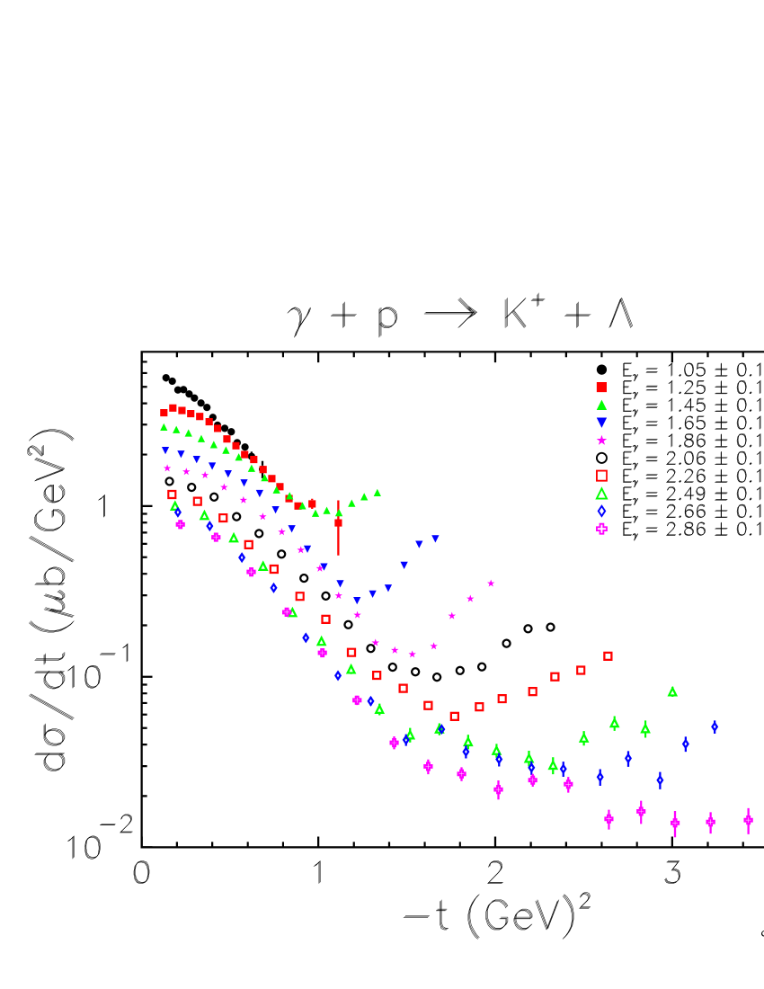
Figure 22: (Color online) The entire $\gamma+p\rightarrow K^{+}+\Lambda$ data set shown as $d\sigma/dt$ vs. $-t$, for ten bands of photon energy with $\Delta E_{\gamma}=0.20$ GeV. No scaling was applied.

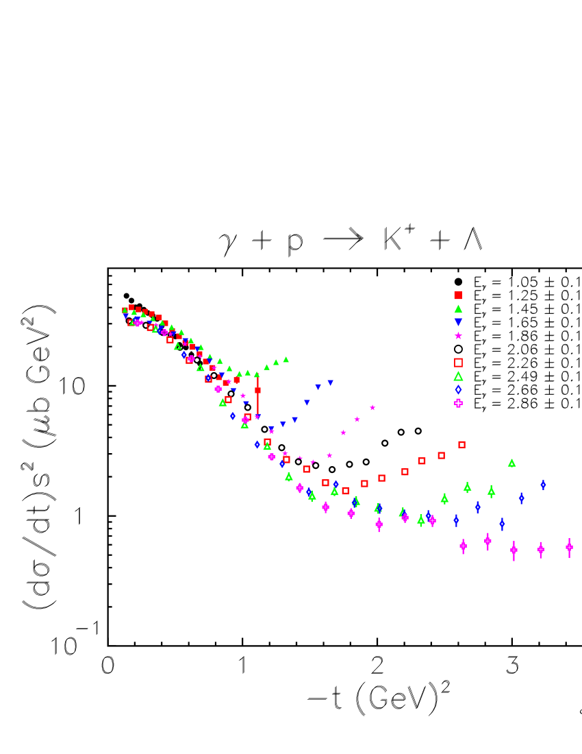
Figure 23: (Color online) The entire $\gamma+p\rightarrow K^{+}+\Lambda$ data set shown as $d\sigma/dt$ vs. $-t$, for ten bands of photon energy with $\Delta E_{\gamma}=0.20$ GeV. The cross sections were scaled by $s^{2}=W^{4}$, resulting in a well-defined band of data for low $-t$ values.

The cross section $d\sigma/dt$ for the $\Sigma^{0}$ channel is shown in Fig. 24. In this case, the data do not fall in monotonically shifting contours as $E_{\gamma}$ increases, as was the case for the $\Lambda$ in Fig. 22. Instead, a more nucleon-resonance dominated picture is suggested by the crossing of the bands of data points. This is emphasized again in Fig. 25 that shows the $s^{2}$ scaled cross sections, which in this case do not form a tight band of points. There is no consistent trend toward a flattening of the slope, as was the case in $K^{+}\Lambda$ production; in the previously cited theory lag1 this is because in $K^{+}\Sigma^{0}$ production the $K$ plays little role compared to $K^{*}$ since $g_{K\Sigma N}<g_{K\Lambda N}$. Furthermore, the large “resonant” rise in the $\Sigma^{0}$ cross section near $W=1.90$ GeV is serving to cover up any simple $t$-channel behavior for this hyperon.

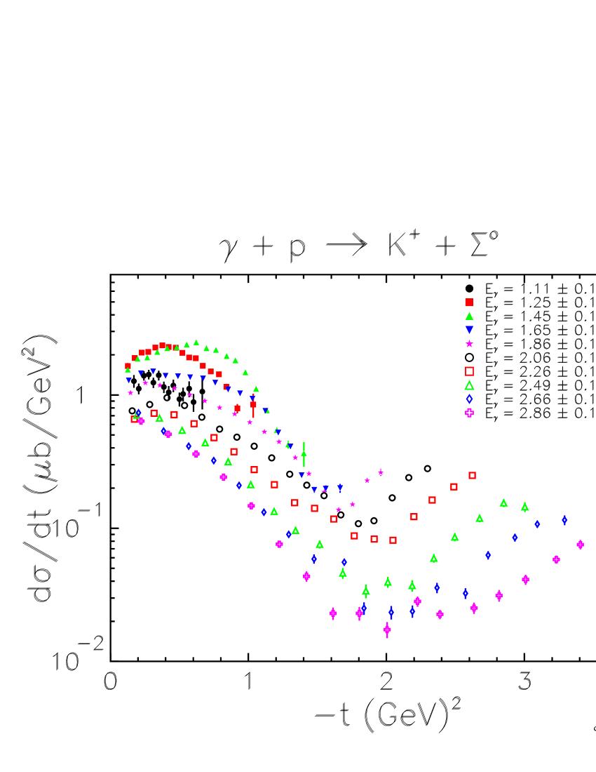
Figure 24: (Color online) The entire $\gamma+p\rightarrow K^{+}+\Sigma^{0}$ data set shown as $d\sigma/dt$ vs. $-t$, for ten bands of photon energy with $\Delta E_{\gamma}=0.20$ GeV. No scaling was applied.

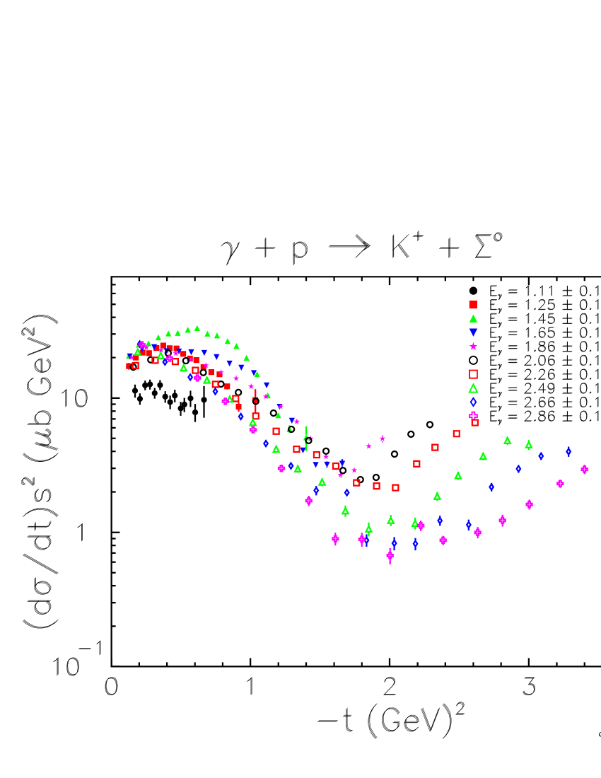
Figure 25: (Color online) The entire $\gamma+p\rightarrow K^{+}+\Sigma^{0}$ data set shown as $d\sigma/dt$ vs. $-t$, for ten bands of photon energy with $\Delta E_{\gamma}=0.20$ GeV. The cross sections were scaled by $s^{2}=W^{4}$, showing a less well-defined band of points than in the $K^{+}\Lambda$ case.

At high enough energies, it is expected, however, that the $\Sigma^{0}$ cross section should also behave as expected by $t$-channel dominance. In Fig. 26 we show the subset of the data from the previous figure for $E_{\gamma}>2.39$ GeV, where the scaling by $s^{2}$ does seem to work. We note that this is well above the large “$\Delta$” peak in the total cross section, Fig. 21, and spans the range where the Regge calculation lag1 ; lag2 is successful in explaining these data.

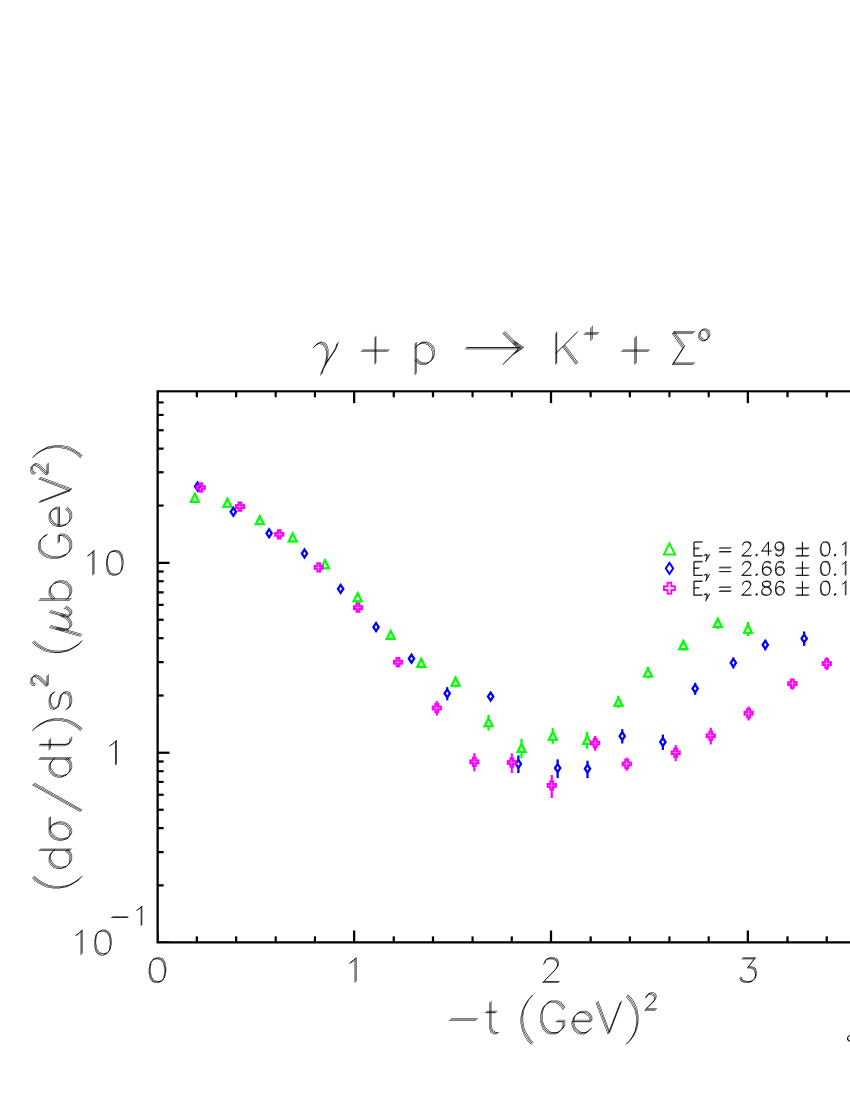
Figure 26: (Color online) The $\gamma+p\rightarrow K^{+}+\Sigma^{0}$ data shown as $d\sigma/dt$ vs. $-t$, for the top three bands of photon energy with $\Delta E_{\gamma}=0.20$ GeV. The cross sections were scaled by $s^{2}=W^{4}$, showing that for the highest energies the same scaling phenomenon is apparent.

VII CONCLUSIONS

In summary, we present results from an experimental investigation of $\Lambda$ and $\Sigma^{0}$ hyperon photoproduction from the proton in the energy range where nucleon resonance physics should dominate. We provide the to-date largest body of data for these reactions in coverage over energy and meson angle. Our $K^{+}\Lambda$ cross section results reveal an interesting $W$-dependence: double-peaked at forward and backward angles, but not at central angles. We see that the structure near $W=1.9$ GeV shifts in position and shape from forward to backward angles. This finding cannot be explained by a $t$-channel Regge-based model or by the addition of a single new resonance in the $s$ or $u$ channel. The $\Sigma^{0}$ results confirm a single large maximum in the cross section near 1.9 GeV, with weak indications of more structure between 2.0 and 2.1 GeV. The results are in fair or good agreement with several older experiments. For the $K^{+}\Lambda$ case we see that a phenomenological scaling of the $t$-dependence of the cross section by $s^{2}$ is quite successful in describing the full range of forward-angle data, and that this scaling does not work as well for the $K^{+}\Sigma^{0}$ data. Our results show that hyperon photoproduction can reveal resonance structure previously “hidden” from view, thereby improving our understanding of nucleonic excitations in the higher mass region where data are sparse. Comprehensive partial wave analysis and amplitude modeling for these results can therefore be hoped to firmly establish the mass and possibly the quantum numbers of these states.

- (1) J. W. C. McNabb, R. A. Schumacher, L . Todor (CLAS Collaboration), et al., Phys. Rev. C 69 042201(R) (2004).
- (2) S. Capstick and W. Roberts, Phys. Rev. D58, 074011 (1998), and references therein.
- (3) S. Eidelman et al., Phys. Lett. B592, 1 (2004).
- (4) See for example: E. Klempt, nucl-ex/0203002, and references therein.
- (5) T. Mart, C. Bennhold, H. Haberzettl and L. Tiator, “KaonMAID 2000” at www.kph.uni-mainz.de/MAID/kaon/kaonmaid.html.
- (6) T. Mart and C. Bennhold, Phys. Rev. C61, 012201 (2000); C. Bennhold, H. Haberzettl, and T. Mart, nucl-th/9909022 and Proceedings of the 2nd Int’l Conf. on Perspectives in Hadronic Physics, Trieste, S. Boffi, ed., World Scientific, (1999).
- (7) U. Löring, B. Ch. Metsch, and H. R. Petry, Eur. Phys. J. A 10, 395 (2001).
- (8) M. Q. Tran et al., Phys. Lett. B445, 20 (1998); M. Bockhorst et al., Z. Phys. C63, 37 (1994).
- (9) B. Saghai, nucl-th/0105001, AIP Conf. Proc. 59, 57 (2001). See also: J. C. David, C. Fayard, G. H. Lamot, and B. Saghai, Phys. Rev. C53, 2613 (1996); curve by private communication.
- (10) S. Janssen, J. Ryckebusch, D. Debruyne, and T. Van Cauteren, Phys. Rev C65, 015201 (2001); S. Janssen et al., Eur. Phys. J. A 11, 105 (2001); curves via private communication.
- (11) S. Janssen, D. G. Ireland, and J. Ryckebusch, Phys. Lett. B 562, 51 (2003) [arXiv:nucl-th/0302047].
- (12) D. G. Ireland, S. Janssen, and J. Ryckebusch, Nucl. Phys. A 740 (2004) 147.
- (13) R. G. T. Zegers et al. [LEPS Collaboration], Phys. Rev. Lett. 91, 092001 (2003) [arXiv:nucl-ex/0302005].
- (14) R. M. Mohring et al. [E93018 Collaboration], Phys. Rev. C 67, 055205 (2003) [arXiv:nucl-ex/0211005].
- (15) G. Penner and U. Mosel, Phys. Rev. C 66, 055212 (2002).
- (16) W. T. Chiang, Ph.D. Thesis, University of Pittsburgh (2000) (unpublished); Wen-Tai Chiang, B. Saghai, F. Tabakin, T. S. H. Lee, Phys. Rev. C 69, 065208 (2004).
- (17) V. Shklyar, H. Lenske, and U. Mosel, Phys. Rev. C 72, 015210 (2005) [arXiv:nucl-th/0505010].
- (18) K.-H. Glander et al., Eur. Phys. J. 19, 251 (2004).
- (19) A. V. Sarantsev, V. A. Nikonov, A. V. Anisovich, E. Klempt, and U. Thoma, arXiv:hep-ex/0506011.
- (20) M. Guidal, J.-M. Laget, and M. Vanderhaeghen, Nucl. Phys. A627, 645 (1997).
- (21) M. Guidal, J.-M. Laget, and M. Vanderhaeghen, Phys Rev. C61, 025204 (2000).
- (22) D. Sober et al., Nucl. Instrum. Methods A440, 263 (2000).
- (23) B. Mecking et al., Nucl. Instrum. Methods A503, 513 (2003), and references therein.
- (24) R.A. Arndt, W.J. Briscoe, I.I. Strakovsky, and R.L. Workman, Phys. Rev. C66, 055213 (2002).
- (25) J. W. C. McNabb, Ph.D. Thesis, Carnegie Mellon University (2002) (unpublished). Available at www.jlab.org/Hall-B/general/clas_thesis.html.
- (26) R. K. Bradford, Ph.D. Thesis, Carnegie Mellon University (2005) (unpublished). Available at www.jlab.org/Hall-B/general/clas_thesis.html.
- (27) The CLAS Database collects all data from CLAS. It is reachable via http://clasweb.jlab.org/physicsdb.
- (28) Text file available by sending email request to schumacher@cmu.edu.
- (29) H. M. Brody, A. M. Wetherell, and R. L. Walker, Phys. Rev. 119, 1710 (1960).
- (30) C. W. Peck, Phys. Rev. 135, B830 (1964).
- (31) D. E. Groom and J. H. Marshall, Phys. Rev. 159, 1213 (1967).
- (32) P. L. Donoho and R. L Walker, Phys. Rev. 112, 981 (1958); Phys. Rev. 107, 1198 (1957);
- (33) R. L. Anderson et al., Phys. Rev. Lett. 9, 131 (1962); also: Phys. Rev. 123, 1003 (1961).
- (34) H. Thom, Phys Rev. 151, 1322 (1966); H. Thom, Phys. Rev. Lett. 11, 432 (1963).
- (35) A. Bleckmann et al., Z. Phys. 239, 1 (1970).
- (36) P Feller, D. Menze, U. Opara, W. Schulz, and W. J. Schwille, Nucl Phys. B39, 413 (1972).
- (37) D. Decamp et al., Preprint LAL 1236, Orsay (1970); Th. Fourneron, LAL 1258, Orsay (1971).
- (38) H. Göing, W. Schorsch, J. Tietge, and W. Weilnböck, Nucl. Phys. B26, 121 (1971).
- (39) T. Fujii et al. Phys. Rev. D 2, 439 (1970).
- (40) “Photoproduction of Elementary Particles,” Landolt-Börnstein, New Series I/8, editted by H. Genzel, P. Joos, and W. Pfeil, Landolt-Börnstein, New Series I/8 (Springer Verlag, NY) (1973).
- (41) The values were read from the published graphs.
- (42) R. Erbe et al. (ABBHHM Collaboration) Phys. Rev. 188, 2060 (1969); data tabulated in “Numerical data and Functional Relationships in Science and Technology”, editted by H. Schopper, Landolt-Börnstein, New Series I/12b (Springer Verlag, NY), 388.
- (43) A. M. Boyarski et al., Phys. Rev. Lett. 22, 1131 (1969).
- (44) See for example: D. H. Perkins, Introduction to High Energy Physics, 2nd Ed., Addison Wesley, pp 166 (1982).