Precision Measurement of the ²⁹Si, ³³S, and ³⁶Cl Binding Energies

Abstract

The binding energies of ²⁹Si, ³³S, and ³⁶Cl have been measured with a relative uncertainty $<0.59\times 10^{-6}$ using a flat-crystal spectrometer. The unique features of these measurements are 1) nearly perfect crystals whose lattice spacing is known in meters, 2) a highly precise angle scale that is derived from first principles, and 3) a gamma-ray measurement facility that is coupled to a high flux reactor with near-core source capability. The binding energy is obtained by measuring all gamma-rays in a cascade scheme connecting the capture and ground states. The measurements require the extension of precision flat-crystal diffraction techniques to the 5 to 6 MeV energy region, a significant precision measurement challenge. The binding energies determined from these gamma-ray measurements are consistent with recent highly accurate atomic mass measurements within a relative uncertainty of $4.3\times 10^{-7}$. The gamma-ray measurement uncertainties are the dominant contributors to the uncertainty of this consistency test. The measured gamma-ray energies are in agreement with earlier precision gamma-ray measurements.

I Introduction

Nuclear binding energy measurements are of interest because they are accurately related to atomic mass measurements. This relationship provides a means to check the results in one precision measurement field against related results obtained in another precision measurement field. Because the experimental techniques used in the two fields are very different, this check has the potential to reveal systematic errors associated with either measurement.

The synergism between binding energy and atomic mass measurements can be demonstrated by considering a typical neutron capture reaction $n+{}^{A}\text{X}\rightarrow{}^{A+1}\text{X}+\gamma$’s which leads to the following equation involving atomic masses and the binding energy,

$$m(n)+m(^{A}\text{X})=m(^{A+1}\text{X})+S_{n}\,.$$ (1)

Atomic masses $m$ are measured in atomic mass units while the binding energy of ${}^{A+1}\text{X}$, $S_{n}$, is obtained from gamma-ray wavelengths measured in meters. The binding energy in meters can be converted to atomic mass units using the molar Planck constant, $N_{A}h$, divided by the speed of light, $c$ Deslattes and Kessler, Jr. (1979). This combination of constants is known with a relative uncertainty of $6.7\times 10^{-9}$, an accuracy which does not limit the test implied by Eq. (1), given the presently available accuracy in atomic mass and binding energy measurements Mohr and Taylor .

New precision measurements of the ²⁹Si, ³³S, and ³⁶Cl binding energies have been made using a flat crystal spectrometer. This spectrometer measures the wavelengths of the gamma-ray photons using crystals whose lattice spacings are known in meters and an angle scale that is derived from first principles. Thus, the measured wavelengths are on a scale consistent with optical wavelengths and the SI definition of the meter. The binding energies of these three nuclei are in the 8.5 to 8.6 MeV range and are obtained by measuring lower energy lines that form a cascade scheme connecting the capture and ground states. For all three nuclei, the cascade scheme with the most intense transitions includes a gamma-ray with energy $>4.9$ MeV. Such high energies present a significant measurement challenge for gamma-ray spectroscopy because the Bragg angles are $<0.1^{\circ}$ and the diffracted intensity is rather small (a few s^-1 or less).

II The ²⁹Si, ³³S, and ³⁶Cl Decay Schemes

In Fig. 1 we show partial decay schemes for ²⁹Si, ³³S, and ³⁶Cl containing the transitions that were measured in these binding energy determinations. The values in parentheses are the number of gamma-rays emitted per 100 captures Lone et al. (1981). The reactions, the thermal neutron capture cross sections, and the nominal energies of the measured gamma-rays are listed in Table 1 Firestone et al. (1996). Because ³⁵Cl has the largest thermal neutron capture cross section of any light nuclei, the ³⁶Cl binding energy was measured first. The experience gained in increasing the crystal reflectivity and lowering the background during the ³⁶Cl measurement proved to be very valuable in the measurement of the weaker ²⁹Si and ³³S transition energies. In addition, a larger than expected dependence of the angle calibration on the environment was noted during the Cl measurements which led to more frequent angle calibrations during the ²⁹Si and ³³S measurements. The ²⁹Si measurement is particularly difficult because the 4934 keV line is emitted while the nucleus is recoiling following the emission of the 3539 keV line. Thus, the 4934 keV profile is significantly Doppler broadened which decreases the accuracy with which the Bragg angle can be determined. In each of these nuclei there are other less intense transitions that connect the capture and ground states. However, the measurement uncertainty of these weaker lines will be so large that their contribution to the binding energy determination will be small. As the stability of the spectrometer improves and techniques to measure weaker lines are developed, these weaker lines may be used for future binding energy determinations.

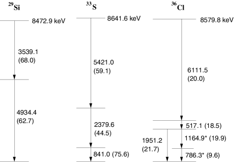
Figure 1: Partial decay schemes for ²⁹Si, ³³S, ³⁶Cl showing the transitions that were measured in this study. The numbers in parentheses are the number of gammas per 100 neutron captures. The transitions marked with asterisks in Cl were not used to deduce binding energies.

Table 1: Reactions, cross-sections, and nominal energies associated with the binding energy determinations.

Nuclide	Reaction	Cross-section	Nominal	Energies measured
		($\times 10^{-28}$ m2)	binding energy	(keV)
			(keV)
29Si	$n+{}^{28}\text{Si}\rightarrow{}^{29}\text{Si}+\gamma$	$0.177$	8473	3539, 4934
33S	$n+{}^{32}\text{S}\rightarrow{}^{33}\text{S}+\gamma$	$0.53$	8642	841, 2380, 5421
36Cl	$n+{}^{35}\text{Cl}\rightarrow{}^{36}\text{Cl}+\gamma$	$43.6$	8580	517, 786, 1951, 6112

III Experiment

The measurements were made at the Institut Laue-Langevin (ILL) using the GAMS4 flat crystal spectrometer. A detailed description of this facility is available to the interested reader in Ref. Kessler, Jr. et al., 2001. The discussion of the experiment given here will be limited to those aspects that are peculiar to these measurements. This spectrometer is located on the reactor floor at the exit of a through-tube that has facilities to transport and hold sources next to the reactor core. Five beamtime allocations were devoted to these binding energy measurements. Chlorine was measured in February 1997 and September 1997. Sulfur was measured in September–October 1998 and April–May 1999. Silicon was measured in October–November 2000. The first measurement cycle (February 1997) served as a proof of the capability of the facility to determine binding energies. In retrospect, it was necessary to exclude all data taken during this cycle from the final results because the experimental conditions were not sufficiently controlled.

The stability of the angle calibration of the spectrometer has been a particularly troublesome experimental problem. Throughout the extended period of the measurements reported here, the angle calibration of the spectrometer has been measured many times, both during and between the binding energy measurements. However, at the start of these measurements we were not aware of the dependence of the angle calibration on the humidity and did not perform calibrations as frequently. From 1998 forward, more frequent calibrations have provided a means to obtain more accurate angle calibrations. Following considerable data analyses aimed at mining the angle calibrations and gamma-ray measurements for maximum information, we have reached the following conclusions concerning the angle calibration: a relative uncertainty due to the angle calibration of $\approx 0.4\times 10^{-6}$ should be included in each measurement period. More details concerning the angle calibration are given in Sec. IV.

At the start of the experiment, it was our intention to measure the 786 keV and 1165 keV lines in Cl to provide a cascade cross-over verification of the 1951 keV line. Because of beamtime restrictions and angle calibration difficulties, this cascade cross-over verification was not realized. However, a very limited data set for the 786 keV line was recorded and used to provide a value for the wavelength of this transition.

III.1 Sources

The source handling mechanism can accommodate three sources that are positioned one behind the other on the beam axis, a line connecting the source region and the center of the axis of rotation of the first crystal. The source material was placed in thin-walled graphite holders that are supported on “V”s for precise positioning. Two sizes of graphite holders were used. For the two chlorine and first sulfur measurements, the inside volume of the source holder was 2 mm $\times$ 50 mm $\times$ 25 mm with the 2 mm $\times$ 50 mm surface facing the spectrometer. For the second sulfur and silicon measurement, the inside volume was 3.5 mm $\times$ 50 mm $\times$ 25 mm with the 3.5 mm $\times$ 50 mm surface facing the spectrometer. The neutron flux at the source position is $\approx 5.5\times 10^{14}$ cm^-2 s^-1. In Table 2 the sources, the source masses, and the estimated activities for each of the measurements are given. The sources that are used are extremely active to compensate for the small effective solid angle (high resolution) of the spectrometer.

Table 2: Sources, source masses, and estimated activities for each of the measurements.

Nuclide	Measurement	Source	Source mass	Estimated activity
	dates		(g)	($\times$ 1013 Bq)
29Si	Oct–Nov 2000	Si single crystal	$13.4$	$2.6$
33S	Sept–Oct 1998	ZnS single crystal	$8.1$	$1.4$
33S	April–May 1999	ZnS polycrystal	$16.8$	$2.9$
36Cl	Feb 1997	NaCl	$4.5$	$85.4$
36Cl	Sept 1997	NaCl	$4.5$	$85.4$

III.2 Spectrometer

The critical component of the gamma-ray facility is a double flat crystal spectrometer that has three unique capabilities that are very important for the accurate measurement of pico-meter wavelengths. First, the diffraction crystals are highly perfect specimens whose lattice spacing is measured on a scale consistent with the SI definition of the meter. Second, the diffraction angles are measured with sensitive Michelson angle interferometers which are calibrated using an optical polygon Kessler, Jr. et al. (2001). The angle calibration is based on the fact that the sum of the external angles of the polygon equals $360^{\circ}$. Third, the gamma-ray beam collimation is sufficient to permit the measurement of very small diffraction angles ($<0.05^{\circ}$). The GAMS4 facility is a precision metrology laboratory with the usual attention to vibration isolation, temperature control, and environmental monitoring.

Because descriptions of the profile recording and the angle calibration that follow assume some knowledge of the angle measuring system of the spectrometer, a few details concerning the angle interferometers are provided. Each of the two Michelson angle interferometers contains two corner cube retro-reflectors that are rigidly attached to the crystal rotation table. As the crystal rotates, the path length of one arm of the interferometer increases while the path length of the other arm decreases. The angles are measured in whole and fractional interferometer fringes with 1 fringe $\approx 7.8\times 10^{-7}$ rad. An interferometer fringe can be divided into $\approx 1000$ parts ($\approx 7.8\times 10^{-10}$ rad). The arm that supports the retro-reflectors is made out of low expansion invar in order to reduce the temperature dependence of the angle interferometer. Nevertheless, the temperature of the corner cube arm must be taken into account when converting interferometer fringe values into angles (see Sec. IV). Because the interferometers are in the laboratory environment, all angle fringe measurements must be corrected to standard pressure, temperature, and humidity conditions.

III.3 Crystals

The gamma-rays measured in this study were diffracted by nearly perfect silicon crystals used in transmission geometry. All of the crystals were cut so that the (220) family of planes was available for diffraction and have a shape and mounting identical to the crystal shown in Fig. 7, Ref. Kessler, Jr. et al., 2001. Because of the large spread in energy of the gamma-rays, two different sets of crystals were used. The first set, called ILL2.5, consisted of two crystals of nearly equal thickness ($\approx 2.5$ mm), and are the same crystals used for the measurement of the deuteron binding energy Kessler, Jr. et al. (1999). The raw material for these crystals was obtained from the Solar Energy Research Institute dis . The second set, called ILL4.4&6.9, consisted of two crystals of unequal thickness ($\approx 4.41$ mm and $\approx 6.95$ mm) manufactured from raw material obtained from Wacker dis . The ILL2.5 crystals were used for the lower energy lines (S 841 keV and 2380 keV and the Cl 517 keV, 786 keV, and 1951 keV lines) and initial measurements of the Cl 6111 keV line. The ILL4.4&6.9 crystals were used for the higher energy lines (Si 3539 keV and 4934 keV, S 5421 keV, and Cl 6111 keV lines). The dependence of integrated reflectivity on crystal thickness and energy is discussed in more detail in Section 11, Ref. Kessler, Jr. et al., 2001. Each line was measured in at least two orders that were chosen on the basis of high reflectivity and small diffraction width. In Table 3 the crystal configurations that were used for each energy are given along with the nominal Bragg angles.

Table 3: Crystals, crystal orders, and nominal Bragg angles for the various energies.

Nuclide	Energy	Crystals	A crystal		B crystal
	(keV)		order-m	$\text{Bragg angle}^{\circ}$	order-n	$\text{Bragg angle}^{\circ}$
29Si	3539	ILL4.4&6.9	$1$	$0.052$	2,-2	$0.105$
	3539	ILL4.4&6.9	$1$	$0.052$	3,-3	$0.157$
	4934	ILL4.4&6.9	$1$	$0.037$	$1$	$0.037$
	4934	ILL4.4&6.9	$1$	$0.037$	2,-2	$0.075$
33S	841	ILL2.5	$1$	$0.220$	1,-1	$0.220$
	841	ILL2.5	$1$	$0.220$	3,-3	$0.660$
	2380	ILL2.5	$1$	$0.078$	$1$	$0.078$
	2380	ILL2.5	$1$	$0.078$	2,-2	$0.155$
	2380	ILL2.5	$1$	$0.078$	$-3$	$0.233$
	5421	ILL4.4&6.9	$1$	$0.034$	$1$	$0.034$
	5421	ILL4.4&6.9	$1$	$0.034$	2,-2	$0.068$
	5421	ILL4.4&6.9	$1$	$0.034$	3,-3	$0.102$
36Cl	517	ILL2.5	$2$	$0.716$	2,-2	$0.716$
	517	ILL2.5	$2$	$0.716$	3,-3	$1.074$
	786	ILL2.5	$1$	$0.235$	1,-1	$0.235$
	1951	ILL2.5	$1$	$0.095$	2,-2	$0.190$
	1951	ILL2.5	$2$	$0.190$	2,-2	$0.190$
	6111	ILL2.5, ILL4.4&6.9	$1$	$0.030$	$1$	$0.030$
	6111	ILL2.5, ILL4.4&6.9	$1$	$0.030$	$2$	$0.061$
	6111	ILL2.5, ILL4.4&6.9	$1$	$0.030$	3,-3	$0.091$

In the past our approach to the determination of the unknown lattice spacing of diffraction crystals combined two types of crystal lattice spacing measurements: 1) absolute lattice parameter measurements in which the lattice parameter of a particular Si crystal is compared to the wavelength of an ¹²⁷I₂ stabilized laser and 2) lattice comparison (relative) measurements in which the small lattice spacing difference between known and unknown crystal samples was measured. Absolute lattice parameter measurements have been published by researchers at the Physikalisch-Technische Bundesanstalt (PTB) in 1981 Becker et al. (1981), at the Istituto di Metrologia “G. Colonnetti” (IMGC) in 1994 Basile et al. (1994), and at the National Measurement Institute of Japan (NMIJ) in 1997 Nakayama and Fujimoto (1997). Lattice comparison measurements have been made at the PTB Windisch and Becker (1990) and the National Institute of Standards and Technology (NIST) Kessler et al. (1994, 1997). In Ref. Kessler, Jr. et al., 1999 the above approach applied to the determination of the lattice parameter of the ILL2.5 crystals is described in detail using the data that was available in 1999. Although an early 2004 publication contains improved absolute lattice parameter measurements from IMGC and NMIJ Cavagnero et al. (2004a), the authors have since published an erratum and advised us not to use these results Cavagnero et al. (2004b).

One of the authors of the 1998 and 2002 CODATA Recommended Values of the Fundamental Physical Constants has recommended an alternate approach for determining lattice parameters values for the crystals used in these measurements pri (a). In the adjustment of the fundamental physical constants, absolute and relative lattice parameter measurements are used in a consistent way to arrive at recommended output values. One of the output values is the lattice parameter of an ideal single crystal of naturally occurring Si free of impurities and imperfections. Since the relative lattice parameter measurements connecting the ILL2.5 crystals to the PTB, IMGC, and NMIJ absolute lattice parameter crystals in Ref. Kessler, Jr. et al., 1999 are included in the input data, the value of the lattice parameter of the ILL2.5 crystal is an unpublished output of the adjustment process. In the 2002 CODATA adjustment Mohr and Taylor only the NMIJ absolute lattice parameter value was used as input based on preliminary measurements that were eventually published in Ref. Cavagnero et al., 2004a. Because these measurements are now known to be in error, the best estimate for the lattice parameter of the ILL2.5 crystal must be taken from the 1998 CODATA adjustment Mohr and Taylor (2000) and is d(220) ILL2.5 = $1.920155822(57)\times 10^{-10}$ m at $\vartheta=22.5~{}^{\circ}$C in vacuum (relative uncertainty of $3.0\times 10^{-8}$). We prefer to arbitrarily increase the relative uncertainty to $5.0\times 10^{-8}$ to account for the present inconsistency of absolute and relative lattice parameter results and the variation of the lattice spacing within the raw material from which the crystals are manufactured.

To obtain a value for the lattice parameter of the ILL4.4&6.9 crystal, the NIST lattice comparison facility was used to measure the lattice spacing difference between the ILL2.5 and ILL4.4&6.9 crystals. The directly measured relative lattice parameter difference is $(\text{ILL2.5}-\text{ILL4.4\&6.9})/\text{ILL2.5}=4.0\times 10^{-8}$. By combining this relative lattice parameter measurement with the above absolute value for d(220) ILL2.5 yields the value for d(220) ILL4.4&6.9 that is given in Table 4. The reasons for preferring this approach for determining lattice parameter values over the approach that was used in Ref. Kessler, Jr. et al., 1999 are all lattice parameter measurements included in the 1998 CODATA adjustment are used in a consistent way to obtain a value for d(220) ILL2.5 and only one direct lattice comparison is needed to obtain a value for d(220) ILL4.4&6.9.

Table 4: Lattice spacing of ILL2.5 and ILL4.4&6.9 crystals. The ILL2.5 value is an unpublished output of the CODATA adjustment process. The NIST lattice comparison facility was used to measure the lattice spacing difference between the ILL2.5 and ILL4.4&6.9 crystals.

$d$(220) ILL2.5 (m)	$1.920155822(96)\times 10^{-10}$
$(\text{ILL2.5}-\text{ILL4.4\&6.9})/\text{ILL2.5}$	$4.0(1.0)\times 10^{-8}$
$d$(220) ILL4.4&6.9 (m)	$1.920155745(96)\times 10^{-10}$

However, it is instructive to compare the d(220) values given in Table 4 to d(220) values obtained with the procedure used in Ref. Kessler, Jr. et al., 1999. The relative difference between the values for d(220) ILL2.5 given in Table 4 and in Ref. Kessler, Jr. et al., 1999 is $5.2\times 10^{-8}$. The deuteron binding energy and the neutron mass values given in Ref. Kessler, Jr. et al., 1999 must be corrected for this change. In order to use the Ref. Kessler, Jr. et al., 1999 approach to determine the ILL4.4&6.9 lattice spacing, the ILL 4.4&6.9 crystal was compared to the absolute lattice parameter crystals from PTB, IMGC, and NMIJ. The relative difference between the value for d(220) ILL4.4&6.9 given in Table 4 and the value that is obtained using the Ref. Kessler, Jr. et al., 1999 procedure is $3.9\times 10^{-8}$. These relative differences provide further justification for expanding the relative uncertainty of the lattice parameter measurements to $5\times 10^{-8}$. In addition, the lattice parameter difference between the ILL2.5 and ILL4.4&6.9 crystals can be inferred from the two d(220) values obtained with the Ref. Kessler, Jr. et al., 1999 approach. The implied value of $(\text{ILL2.5}-\text{ILL4.4\&6.9})/\text{ILL2.5}=3.0\times 10^{-8}$ agrees very well with the directly measured value given above and provides further confidence in the lattice parameter results that are used to obtain binding energy measurements.

III.4 Profile recording

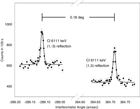
Figure 2: Two representative third order ³⁶Cl profiles along with fitted curves: 6111 keV (1,-3) and (1,3) made with the thick crystals ILL4.4&6.9. The most important fit parameter is the profile centroid. The difference in profile centroids is proportional to the Bragg angle while the numeric mean of the two centroids gives the offset angle between the second crystal diffracting planes and the angle interferometer.

Gamma-ray profiles (intensity vs interferometer fringes) were recorded for the crystal configurations given in Table 3 by scanning the angular position of the second crystal. The profiles consisted of 30 to 45 points with counting times from 30 to 180 seconds per point and were scanned in both the cw and ccw directions. For each data point the interferometer fringe value was reduced to standard atmospheric conditions (pressure, temperature, and humidity) Birch and Downs (1993, 1994). The gamma-ray counts were accumulated in a Ge detector-multichannel analyzer system. The recorded profiles were least squares fit to theoretical dynamical diffraction profiles broadened with a Gaussian function to account for crystal imperfections, vibrations, and thermal and recoil induced motions of the atoms in the source. The use of a single Gaussian function to account for deviations of the recorded profiles from the theoretical dynamical diffraction profiles has been shown to provide reliable peak positions, but is not sufficient to obtain nuclear level lifetimes and recoil velocities from profile width measurements Börner and Jolie (1993). The adjustable parameters in the fit are the position, intensity, background, and Gaussian width contribution. In the fit, the number of counts at fringe value $i$, $n_{i}$, is weighted by $(1/\sqrt{n_{i}})^{2}$. The detector and fitting procedure are described in more detail in Ref. Kessler, Jr. et al., 2001. Two representative profiles are shown in Fig. 2. The profile positions (in interferometer fringes), the most important parameter for the determination of energies, are converted into diffraction angles by using the second-axis angle calibration that is described in the next section.

IV Angle Interferometer Calibration

A complete description of a calibration run can be found in Ref. Kessler, Jr. et al., 2001. As discussed there the formula connecting optical fringes $f$, which are recorded with the rocking curves, and the true interferometer angle $\theta$ is

$$f=K\sin\theta+f_{0}\,,$$ (2)

where $K$ is the instrument calibration constant and $f_{0}$ is an electronic offset. Both terms must be determined experimentally through a calibration procedure. Ideally $K$ would be invariable, however experience shows that $K$ depends on temperature, time, humidity and interferometer laser and alignment.

IV.1 The Global Calibration Procedure

Between September 1997 and May 2002, a period spanning the measurements described in this paper, the GAMS4 spectrometer was calibrated 29 times. Table 5 lists each of these calibrations. The experimentally determined calibration constants (column 5) fit well to a linearized equation

$$K= K_{0}+K_{\vartheta}(\vartheta-26)+K_{d}(d-800)+K_{h}(h-0.35)$$ (3)

$$+K_{\text{laser}}\times\begin{cases}-1&\text{if $d<700$},\\ 1&\text{if $d>700$}\end{cases}$$

where $K=K(\vartheta,d,h)$ is the desired calibration constant, $\vartheta$ is the corner cube arm temperature (^∘C), $h$ is the relative humidity, $d$ is the number of days after 8/31/1997, and $d=700$ corresponds to 8/1/1999 when the interferometer laser was replaced. A least squares fit to the data in Table 5 gives

$$K_{0} =5133462.12\pm 0.59$$

$$K_{\vartheta} =7.5\pm 1.3\;/{}^{\circ}\text{C}$$

$$K_{d} =-0.0059\pm 0.0013$$

$$K_{h} =41.6\pm 3.9$$

$$K_{\text{laser}} =3.13\pm 0.57$$ (4)

where $\vartheta_{\text{avg}}=26~{}^{\circ}$C, $h_{\text{avg}}=0.35$, and $d_{\text{avg}}=800$ (11/9/1999) are average conditions around which the fit is made. This fit is plotted in Fig. 3. The relative standard deviation of the residuals (column 7) is $0.33\times 10^{-6}$. Eqs. (2), (3), and (IV.1) along with values for the profile centroid in fringes, the mean corner cube arm temperature, the mean humidity, and the mean wall time can be used to extract a profile centroid in radians from a single data file. This procedure uses all available calibration data to determine one set of coefficients ($K_{0},K_{\vartheta},K_{d},K_{h},K_{\text{laser}}$) that are assumed valid for all of the data presented in this paper. In the remainder of this paper this procedure is referred to as the Global Calibration.

Table 5: GAMS4 angle calibrations. Each line represents a unique calibration of the spectrometer. Column 1 gives the date of the calibration, column 2 the nuclide being measured, column 3 the calibration-average corner cube arm temperature (^∘C), column 4 the calibration-average relative humidity, column 5 the measured instrument calibration constant $K$, column 6 the measured calibration zero, and column 7 the residuals from a five parameter fit to $K$. The horizontal line indicates the time when the interferometer laser was replaced causing a $(1.22\pm 0.22)\times 10^{-6}$ one time fractional shift in K. “CC” denotes corner cube.

	Nuclide	Avg CC arm	Avg relative			Fit
Date	measured	temp (∘C)	humidity	$K$	$f_{0}$	rel dev$\times 10^{6}$
09/27/1997	36Cl	$25.595$	$0.495$	$5133471.3$	$588.3$	$-0.92$
03/08/1998		$26.272$	$0.317$	$5133463.2$	$-747.7$	$0.01$
03/26/1998		$26.266$	$0.209$	$5133460.1$	$-721.1$	$-0.28$
03/30/1998		$26.256$	$0.308$	$5133462.7$	$-721.2$	$-0.01$
09/26/1998	33S	$26.716$	$0.481$	$5133473.7$	$-547.5$	$-0.30$
10/21/1998	33S	$26.607$	$0.323$	$5133461.8$	$-547.7$	$0.55$
11/05/1998	33S	$26.308$	$0.314$	$5133462.6$	$-203.1$	$-0.11$
11/17/1998	33S	$26.199$	$0.265$	$5133458.1$	$-202.9$	$0.18$
04/13/1999	33S	$26.041$	$0.323$	$5133458.1$	$-186.9$	$0.25$
04/30/1999	33S	$26.194$	$0.536$	$5133466.0$	$-186.9$	$0.64$
05/07/1999	33S	$26.173$	$0.583$	$5133471.2$	$-68.2$	$-0.02$
09/17/1999		$26.492$	$0.464$	$5133474.4$	$-268.2$	$-0.09$
09/19/1999		$26.486$	$0.434$	$5133473.6$	$-268.1$	$-0.18$
09/25/1999		$26.648$	$0.503$	$5133474.1$	$-255.5$	$0.52$
10/05/1999		$26.354$	$0.334$	$5133468.8$	$-254.5$	$-0.26$
10/15/1999		$26.348$	$0.449$	$5133470.3$	$-249.5$	$0.37$
10/18/1999		$26.477$	$0.369$	$5133469.3$	$-249.4$	$0.08$
12/03/1999		$25.493$	$0.257$	$5133454.5$	$-249.5$	$0.59$
07/06/2000		$26.545$	$0.399$	$5133471.3$	$-183.5$	$-0.26$
07/18/2000		$26.474$	$0.390$	$5133468.7$	$-183.4$	$0.05$
10/15/2000	29Si	$26.779$	$0.412$	$5133471.0$	$-253.2$	$0.13$
10/22/2000	29Si	$26.490$	$0.374$	$5133468.5$	$-192.4$	$-0.12$
11/05/2000	29Si	$26.313$	$0.314$	$5133465.4$	$-240.8$	$-0.28$
11/14/2000	29Si	$26.409$	$0.320$	$5133464.8$	$-262.2$	$0.00$
11/28/2000	29Si	$26.302$	$0.312$	$5133462.9$	$-276.1$	$0.14$
10/28/2001		$26.725$	$0.374$	$5133469.1$	$-211.8$	$-0.32$
11/06/2001		$26.619$	$0.316$	$5133465.0$	$-250.0$	$-0.16$
11/12/2001		$26.347$	$0.236$	$5133459.4$	$-250.0$	$-0.13$
05/19/2002		$26.551$	$0.411$	$5133466.7$	$-263.4$	$-0.05$

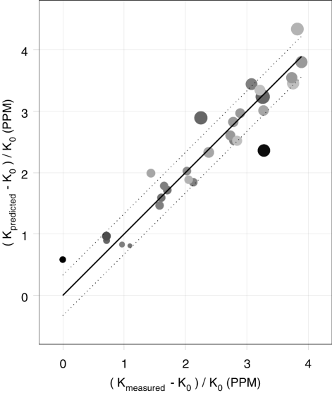
Figure 3: Global fit to 29 GAMS4 calibrations. Predictions from a five parameter global fit [Eq. (3)] are plotted versus measured calibration values. The standard deviation of the relative residuals given in the last column of Table 5 is $0.33\times 10^{-6}$. The dotted lines correspond to $\pm 0.33\times 10^{-6}$ about the fit. Across the data sets the temperature ranges from 25.5 to $26.8~{}^{\circ}$C corresponding to a $1.9\times 10^{-6}$ relative change in K, the relative humidity ranges from 0.21 to 0.58 corresponding to a $3.0\times 10^{-6}$ relative change in K, and 4.6 years separates the first and last measurements corresponding to a $2.0\times 10^{-6}$ relative change in K. The size of the plotted points is proportional to the humidity while darker (lighter) points represent lower (higher) temperatures.

The dependence of $K$ on temperature and time is not unexpected as the physical dimensions of the interferometer corner cube arm can vary with temperature and time in roughly the amounts seen Bergamin et al. (1997); Berthold and Jacobs (1976). The data reveals no dependence of $K$ on atmospheric pressure which is as expected since the interferometer fringe values are reduced to standard atmospheric conditions and the small pressure changes are not likely to alter the dimensions of the interferometer. The relative magnitude of the dependence on interferometer laser ($\approx 1.22\times 10^{-6}$) is somewhat larger than the expected variability in the laser wavelength and is likely due to interferometer alignment. The dependence of $K$ on humidity is unexpected and no definitive cause has been established. In an effort to better understand the dependence of the calibration on the environment, more frequent calibrations were performed as the measurements progressed. As is evident from Fig. 3, there are significant differences between some values of $K_{\text{measured}}$ and $K_{\text{fit}}$. These differences prompted us to consider alternate calibration procedures.

IV.2 Other Calibration Procedures

For the later measurement cycles, multiple calibrations were performed: ³³S 1998 - 4, ³³S 1999 - 3 and ²⁸Si 2000 - 5. Since these calibrations were dispersed throughout the measurement cycle, it is possible to interpolate between the measured calibrations using spline fitting to obtain calibration constant values for converting profile data in fringes to angles. This procedure assumes that each of the recorded angle calibrations is valid and the angle calibration varies smoothly with time during the measurement cycle. Although the individual calibration values within a measurement cycle are dependent on temperature, humidity, and day number, the spline fitting uses only the individual calibration values and assumes no explicit dependence on temperature, humidity or day number. We have called this calibration procedure the Spline Calibration. It uses only the calibration information obtained during a given measurement cycle to analyze the wavelength data recorded in that cycle. The ³³S and ²⁹Si data were analyzed using the spline calibration and the relative difference between wavelengths obtained with the global and spline calibration procedures is $\approx 0.2\times 10^{-6}$. Since only one calibration was recorded during the ³⁶Cl 1997 measurement cycle, the spline calibration could not be applied to this data. This led us to a third calibration procedure called the Local-Global Calibration.

In the local-global calibration, the calibrations that were performed in a particular measurement cycle are given a more significant role in the determination of $K(\vartheta,d,h)$ for that measurement cycle. First, $K_{\vartheta}$, $K_{d}$, $K_{h}$, and $K_{\text{laser}}$ are taken as given in Eq. (IV.1) since these coefficients are not expected to change with time and a global fit provides the best estimate of these coefficients. Next the subset of calibrations performed in each measurement cycle are fit to the equation

$$K= K_{0}+7.5(\vartheta-26)-0.0059(d-800)$$ (5)

$$+41.6(h-0.35)+3.13\times\begin{cases}-1&\text{if $d<700$},\\ 1&\text{if $d>700$}\end{cases}$$

to obtain independent values of $K_{0}$ for each measurement cycle. All of the ³³S and ²⁹Si data were analyzed using the local-global calibration procedure and the relative difference between wavelengths obtained with global and local-global calibration procedures is $\approx 0.3\times 10^{-6}$. The ³⁶Cl data were also analyzed using the local-global calibration procedure and show significantly larger relative differences ($\approx 0.9\times 10^{-6}$) between wavelengths obtained with the global and local-global calibration procedures. These large differences result from recording only one calibration during the ³⁶Cl measurement cycle and from the fact that this particular calibration is the most discrepant point in the global fit of Fig. 3.

Consideration of these alternate calibration procedures did not provide sufficient evidence to make a “best” calibration procedure choice. All of the wavelength and energy values reported in this paper were obtained using the global calibration procedure. Our reasons for choosing this procedure are 1) all of the available data can be analyzed using one procedure and 2) this procedure makes the maximum use of the available calibration data.

IV.3 Calibration Uncertainty

Although consideration of three calibration procedures did not lead to a clear “best” procedure, this exercise does provide an estimate of the calibration uncertainty. The variation of wavelengths obtained with the global, spline and local-global calibration procedures suggests a relative calibration uncertainty of $\text{0.2--0.3}\times 10^{-6}$. A second estimate of the calibration uncertainty is available from the fit used in the global calibration procedure. The standard deviation of the relative residuals given in Table 5 and shown in Fig. 3 is $0.33\times 10^{-6}$ and provides a measure of the quality of the fit and the uncertainty of this calibration procedure. A third estimate of the calibration uncertainty is the variation of the wavelength values obtained in different measurement cycles. In this approach lower energy (larger angles) intense transitions must be used because higher energy (smaller angles) weak transitions have a statistical uncertainty that masks the calibration uncertainty. The 841 keV line in ³³S was measured in 1998 and 1999 and shows a relative excess variation of $0.38\times 10^{-6}$ if the global calibration procedure is used and $0.16\times 10^{-6}$ if the spline calibration is used. In addition, this instrumental set up was used to measure an intense line that does not contribute to the binding energy determinations presented here, namely the 816 keV line in ¹⁶⁸Er. This line was measured in two different measurement cycles, Oct-Nov 2000 and Nov 2003 and shows a relative excess variation of $0.45\times 10^{-6}$ and $0.3\times 10^{-6}$ for the global and spline calibrations, respectively. Although it is difficult to obtain a rigorous calibration uncertainty from these three estimates, we choose to use the above values to arrive at a slightly conservative relative calibration uncertainty of $0.4\times 10^{-6}$. This calibration uncertainty will be combined with the statistical and other systematic uncertainties to obtain final wavelength uncertainties.

V Wavelength measurements

Wavelengths are determined by combining a sequence of profile angle measurements. First the profile centroids and uncertainties in interferometer fringes are converted into angles via Eq. (2). The calibration constant $K$ that appears in this equation has been appropriately corrected for the corner cube arm temperature, the relative humidity, and time. Each of these angles is next corrected for vertical divergence as discussed in Ref. Schnopper, 1965. Typically these corrections are between 2 and $4\times 10^{-7}$ in relative size. For a given energy and configuration the profiles are recorded with the first crystal in a fixed position and the second crystal sequentially in a more and less dispersive position (see Fig. 2). In addition, the data recording sequence includes both cw and ccw rotation of the second crystal. To more concretely illustrate how wavelengths are determined, we use the ³³S 841 keV (1,$-3$), (1,3) measurement as an example. A group of four profiles recorded in the sequence (1,$-3$ cw), (1,3 cw), (1,3 ccw), (1,$-3$ ccw) is used to determine a wavelength value. The four angles associated with the four profiles are fit with the equation

$$\theta(n,t,\vartheta)=\arcsin\left(\frac{n\lambda_{\text{meas}}}{2d(\vartheta)}\right)+\theta_{0}(t)\,,$$ (6)

where $n$ is the diffraction order, $t$ is the time, $\vartheta$ is the crystal temperature, $\lambda_{\text{meas}}$ is the sought after wavelength, $d(\vartheta)$ is the lattice spacing at crystal temperature $\vartheta$ and $\theta_{0}(t)$ represents the potentially time dependent angular offset between the second crystal diffracting planes and the angle interferometer. The symbol $\lambda_{\text{meas}}$ is introduced to indicate that wavelengths determined using this equation are laboratory measured wavelengths (not corrected for recoil); $d(\vartheta)$ is given by

$$d(\vartheta)=d_{\text{$22.5~{}^{\circ}$C, atm}}(1+2.56\times 10^{-6}(\vartheta-22.5))\,,$$ (7)

where $d_{\text{$22.5~{}^{\circ}$C, atm}}$ is the lattice spacing at $22.5~{}^{\circ}$C and atmospheric pressure. The lattice parameter measurements given in Table 4 are specified for vacuum. To obtain the value at the pressure present in the reactor hall ($p\approx 0.987$ atmospheres) it is necessary to use the following transformation

$$d_{\text{$22.5~{}^{\circ}$C}}(p)=d_{\text{$22.5~{}^{\circ}$C, vac}}(1-\epsilon p)\,,$$ (8)

where p is the pressure. In this equation $\epsilon=0.3452\times 10^{-6}$/atmosphere Nye (1957); McSkimin (1953).

In the fit to Eq. (6), the three parameters are the wavelength, a constant angular offset, and a linear temporal offset term (i.e., $\theta_{0}(t)=a+bt$). Each of the four angles $\theta_{i}$ is weighted by $(1/\sigma_{\theta_{i}})^{2}$ where $\sigma_{\theta_{i}}$ is the profile centroid uncertainty. This sequence of profiles is repeated multiple times in at least two different sets of orders (here 29 instances of (1,$-3$), (1,3); 21 instances of (1,$-1$), (1,1); and 1 instance of (1,$-3$), (1,$-1$), (1,1), (1,3)). An uncertainty equal to the standard deviation of the wavelength determinations in a unique set of orders is assigned to each wavelength determination derived from that set of orders. The average wavelength is the weighted mean of all the individual determinations. We find no evidence for an order dependent effect in the wavelength data.

Table 6 gives the nuclide, the nominal energy, the crystals, the total number of Bragg angle measurements and mean wavelength along with the statistical uncertainties in parentheses. The sulfur transitions appear twice because they were measured in 1998 and 1999.

Table 6: Values of the measured wavelengths for the transitions included in the binding energy determinations. The uncertainties are statistical only.

Nuclide	Energy	Crystals	Number of	$\lambda_{\text{meas}}\times 10^{12}$	relative
	(keV)		Bragg angle	(m)	uncertainty
			measurements		$\times 10^{6}$
29Si	3539	ILL4.4&6.9	42	0.350340126(44)	0.13
	4934	ILL4.4&6.9	147	0.25128808(18)	0.70
33S	841	ILL2.5	26	1.47429306(14)	0.09
	2380	ILL2.5	18	0.52103852(30)	0.58
	5421	ILL4.4&6.9	42	0.228730970(63)	0.27
	841	ILL2.5	25	1.47429225(12)	0.08
	2380	ILL2.5	31	0.52103905(23)	0.43
	5421	ILL4.4&6.9	30	0.22873089(13)	0.56
36Cl	517	ILL2.5	15	2.39782393(10)	0.04
	786	ILL2.5	2	1.57681233(83)	0.53
	1951	ILL2.5	12	0.63544928(10)	0.16
	6111	ILL2.5, ILL4.4&6.9	17	0.20288757(10)	0.50

In Table 7, final measured wavelength values and uncertainties are reported (column 3). Four additional sources of uncertainty have been added in quadrature to the statistical uncertainties given in Table 6. These are the calibration uncertainty discussed in Sec. IV and uncertainties associated with the crystal temperature, the vertical divergence of the gamma-ray beam, and the measured lattice spacing. A relative calibration uncertainty of $0.4\times 10^{-6}$ is applied to each energy listed in Table 6. To obtain final sulfur wavelengths and uncertainties it is necessary to add the calibration and statistical uncertainties in quadrature for each sulfur transition before statistically combining the 1998 and 1999 values. This has the effect of reducing the calibration uncertainty for the sulfur lines because they were measured twice. In the case of binding energies where one sums transition energies, the calibration uncertainty is applied to the sum rather than to the constituent transitions; and again, two binding energies are combined to arrive at a final sulfur binding energy. The other three uncertainties are applied to the final transition energies or to the binding energies. An uncertainty in the crystal temperature measurement of 0.05 ^∘C contributes a relative uncertainty of $0.1\times 10^{-6}$. The vertical divergence uncertainty accounts for the possible misalignment of the gamma-ray beam with respect to the plane of dispersion of the spectrometer. A misalignment of 5 mm over a distance of 15 m leads to a relative wavelength uncertainty of $0.06\times 10^{-6}$. This uncertainty is approximately 20% of the size of the correction. From Sec. III.3 and Table 4, the relative crystal lattice spacing uncertainty is $0.05\times 10^{-6}$.

VI Binding energy measurements

In column 4 of Table 7 the corresponding energy equivalent values $E_{\text{meas}}$ are given, where the conversion factor $1\,\text{m}^{-1}=1.23984191(11)\times 10^{-6}$ eV was used Mohr and Taylor .

Table 7: Measured and recoil corrected (transition) wavelengths and energies. Measured values from Ref. Kessler, Jr. et al., 1999 for ²H, which have been adjusted for the adjusted value of d(220) ILL2.5, are included for convenience.

Nuclide	Energy	$\lambda_{\text{meas}}\times 10^{12}$	$E_{\text{meas}}$	$\lambda_{\text{trans}}\times 10^{12}$	$E_{\text{trans}}$	wavelength relative
	(keV)	(m)	(eV)	(m)	(eV)	uncertainty
						$\times 10^{6}$
29Si	3539	0.35034013(15)	$3538966.3(1.6)$	0.35031716(15)	$3539198.3(1.6)$	0.44
	4934	0.25128808(21)	$4933946.3(4.0)$	0.25126511(20)	$4934397.4(4.0)$	0.82
33S	841	1.47429265(47)	$840974.08(28)$	1.47427246(47)	$840985.60(28)$	0.32
	2380	0.52103883(24)	$2379557.6(1.1)$	0.52101864(24)	$2379649.8(1.1)$	0.47
	5421	0.228730944(95)	$5420525.5(2.3)$	0.228710758(95)	$5421003.9(2.3)$	0.42
36Cl	517	2.3978239(10)	$517069.62(22)$	2.3978054(10)	$517073.61(22)$	0.42
	786	1.5768123(11)	$786296.43(53)$	1.5767938(11)	$786305.66(53)$	0.67
	1951	0.63544928(29)	$1951126.47(89)$	0.63543077(29)	$1951183.30(89)$	0.45
	6111	0.20288757(13)	$6110980.2(4.0)$	0.20286906(13)	$6111537.6(4.0)$	0.66
2H	2223	0.557671328(99)	$2223248.44(44)$	0.557341007(99)	$2224566.10(44)$	0.18

The measured wavelength values must be corrected for recoil to obtain wavelength values $\lambda_{\text{trans}}$ whose corresponding energies can be summed to obtain binding energies $S_{n}$. To excellent approximation we account for the recoil by the transformation

$$\frac{hc}{\lambda_{\text{trans}}}=\frac{hc}{\lambda_{\text{meas}}}+\frac{1}{2Mc^{2}}\left(\frac{hc}{\lambda_{\text{meas}}}\right)^{2}\,,$$ (9)

where $M$ is the mass of the decaying nucleus, $h$ is the Planck constant, and $c$ is the speed of light. The second term in Eq. (9) accounts for the loss of energy imparted to the recoiling nucleus. If the decay occurs in flight, there will be a first order Doppler effect. It causes no shift in the central value as long as the motion is isotropic as is expected to be the case here. As discussed in Ref. Ko et al., 1999, two additional terms appear in Eq. (9) in the case of decays from the capture state. First, the kinetic energy of the incident neutron ($\approx 0.057$ eV) must be subtracted from the measured gamma-ray energy. For the three capture gamma-rays measured here (3539 keV in ²⁹Si, 5421 keV in ³³S, and 6111 keV in ³⁶Cl), this effect is less than $0.02\times 10^{-6}$. Second, there is a Doppler term if the incident neutron comes from a particular direction. The relative peak-to-peak amplitude of this term is $\approx 0.6\times 10^{-6}$ for the nuclei being discussed here. The term vanishes if the incident neutron direction is isotropic as is expected to be the case here. The relative uncertainty of the recoil correction is estimated to be no greater than $0.01\times 10^{-6}$. As such it is negligible given the current accuracy of $\lambda_{\text{meas}}$. Values for $\lambda_{\text{trans}}$ and the corresponding energy equivalent $E_{\text{trans}}$ are given in Table 7, column 5 and 6.

To obtain a wavelength equivalent to the binding energy, $\lambda_{\text{be}}$, we sum the reciprocals of the $\lambda_{\text{trans}}$ values for the transitions comprising the binding energy cascade and then convert $\lambda_{\text{be}}$ into atomic mass units using the conversion factor: $1\,\text{m}^{-1}=1.3310250506(89)\times 10^{-15}$ u Mohr and Taylor . Likewise, the binding energy can be expressed in eV by using the $\text{m}^{-1}$ to eV conversion factor given above. Table 8 contains values for the three binding energies of ²⁹Si, ³³S, and ³⁶Cl in meters, atomic mass units and electron volts.

Table 8: Measured binding energies in meters (m), atomic mass units (u) and electron volts (eV). $\lambda_{\text{be}}=\frac{1}{\sum_{i}\frac{1}{\lambda_{\text{trans}_{i}}}}$ is the wavelength of a photon whose energy is equal to the binding energy. Measured values from Ref. Kessler, Jr. et al., 1999 for ²H, which have been adjusted for the adjusted value of d(220) ILL2.5, are included for convenience.

Nuclide	$\lambda_{\text{be}}\times 10^{12}$	$S_{n}\times 10^{3}$	$S_{n}$	wavelength relative
	(m)	(u)	(eV)	uncertainty
				$\times 10^{6}$
29Si	$0.146318275(86)$	$9.0967793(53)$	$8473595.7(5.0)$	$0.59$
33S	$0.143472991(54)$	$9.2771820(35)$	$8641639.8(3.3)$	$0.38$
36Cl	$0.144507180(80)$	$9.2107883(51)$	$8579794.5(4.8)$	$0.55$
2H	$0.557341007(98)$	$2.38816996(42)$	$2224566.10(44)$	$0.18$

VII Discussion

In this section we discuss the consistency of gamma-ray based and atomic mass based binding energy measurements and compare the gamma-ray measurements reported here with other high precision gamma-ray measurements. As discussed in Sec. I, precision atomic mass measurements can be used to determine binding energies. By using atomic mass values from the Atomic Mass Data Center amd ; Audi and Wapstra (1995) and the fundamental constants Mohr and Taylor along with Eq. (1), binding energies primarily based on atomic mass measurements can be determined. However, since the determination of the neutron mass includes a gamma-ray measurement, binding energy determinations based on Eq. (1) are a combination of atomic mass measurements and gamma-ray measurements. This difficulty can be circumvented by expressing $m(n)$ in terms of $m(\text{H})$, $m({}^{2}\text{H})$ and $S_{n}({}^{2}\text{H})$. By making this substitution and rearranging terms, Eq. 1 becomes

$$m({}^{A}\text{X})-m({}^{A+1}\text{X})+m({}^{2}\text{H})-m(\text{H})=$$

$$S_{n}({}^{A+1}\text{X})-S_{n}({}^{2}\text{H})\,.$$ (10)

Since the left and right sides of this equation involve only atomic mass and gamma-ray measurements respectively, this equation is a valid test of the consistency of high-precision atomic mass and gamma-ray measurements.

Recently, new highly accurate values for the left hand side of this equation have been reported for ${}^{A+1}\text{X}$ equal to ²⁹Si and ³³S pri (b). In these measurements the cyclotron frequencies of two different ions simultaneously confined in a Penning trap were directly compared. The measured quantities are the mass ratios $m[{}^{33}\text{S}^{+}]/m[{}^{32}\text{SH}^{+}]$ and $m[{}^{29}\text{Si}^{+}]/m[{}^{28}\text{SiH}^{+}]$ from which, along with the quantity $m({}^{2}\text{H})-2m(\text{H})$, the mass differences on the left hand side of Eq. VII are derived. In Table 9, column 2 the left hand side mass differences for Si and S are given. The relative uncertainties for the Si and S values in column 2 are $7.0\times 10^{-8}$ and $7.3\times 10^{-8}$ respectively.

Values for the right hand side of this equation for ${}^{A+1}\text{X}$ equal to ²⁹Si and ³³S follow directly from the binding energies given in Table 8 and are given in Table 9, column 3. The relative uncertainties for the Si and S values in column 3 are $8.0\times 10^{-7}$ and $5.1\times 10^{-7}$ respectively.

In Fig. 4 the values given in Table 9 are plotted to show the consistency of the atomic mass and gamma-ray measurements. The left and bottom axes are used for ²⁹Si, while the top and right axes are used for ³³S. The scales of the axes have been chosen so that a diagonal line through the plot represents exact consistency between atomic mass and gamma-ray measurements. The plot shows that the quality of the consistency test is limited by the uncertainty of the gamma-ray measurements. For ²⁹Si the two measurements are slightly inconsistent (1.2 $\sigma$), while for ³³S the two measurements agree within the uncertainty (0.4 $\sigma$).

In Table 9, column 4 the fractional difference between the atomic mass and gamma-ray measurements is given along with the weighted average of the Si and S fractional differences. These measurements confirm the consistency of atomic mass and gamma-ray measurements with a relative uncertainty of $4.3\times 10^{-7}$.

Table 9: Consistency of high precision atomic mass and gamma-ray measurements.

${}^{A+1}\text{X}$	$m(^{A}\text{X})-m(^{A+1}\text{X})+m(^{2}\text{H})-m(\text{H})$	$S_{n}(^{A+1}\text{X})-S_{n}(^{2}\text{H})$	relative difference
	(u)	(u)	$(\text{col3}-\text{col2})/\text{col3}\times 10^{7}$
29Si	0.00670861569(47)	0.00670860929(536)	$-9.54(8.02)$
33S	0.00688901053(50)	0.00688901206(351)	$2.22(5.15)$
weighted average
relative difference			$-1.21(4.33)$

The most accurate Si and S gamma-ray energies were measured using Ge(Li) solid state spectrometers. These spectrometers derive an energy scale from gamma-ray standard energies. For high precision comparisons, the published values of the gamma-ray energies need to be adjusted to account for changes in the energy standards. Because a number of energy standards covering a wide energy range are used, the shift in the energy scale for a particular energy is difficult to estimate. Although the procedure that has been used is not rigorous, it is likely sufficient given the accuracy of the published energies. New values for the standards were taken from Ref. Helmer and van der Leun, 2000 or have been determined using atomic mass values from Refs. Mohr and Taylor, , amd, , and Audi and Wapstra, 1995. For ²⁹Si the values of the 3539 keV and the 4945 keV energies in Ref. Raman et al., 1992 have been corrected by $-7$ eV to account for the change in the 2223 keV and the 4945 keV standards produced in the ${}^{1}\text{H}(n,\gamma)$ and ${}^{12}\text{C}(n,\gamma)$ reactions, respectively. For ³³S the values for the 841 keV, 2380 keV, and 5421 keV energies in Ref. Raman et al., 1985 have been corrected by $+8$ eV, $-107$ eV, and $-107$ eV respectively. These corrections account for changes in the 412 keV standard produced in the decay of ¹⁹⁸Au and changes in the 2223 keV, the 4945 keV, and the 10829 keV standards produced in the ${}^{1}\text{H}(n,\gamma)$, the ${}^{12}\text{C}(n,\gamma)$, and the ${}^{15}\text{N}(n,\gamma)$ reactions, respectively. For the low energy Cl lines considerably more precise data exists. In 1985 energy values for some Cl lines were measured using the GAMS4 facility in its early stage of development Kessler, Jr. et al. (1985). These published values also need to be corrected for changes in the fundamental constants Mohr and Taylor and known errors in the lattice spacing of the crystals Deslattes et al. (1987). These corrections to the Cl lines can be made with much more certainty than the corrections to the ²⁹Si and ³³S lines.

Table 10: Comparison of measured gamma-ray energies.

Nuclide	This report	Other references
	$E_{\text{meas}}$	$E_{\text{meas}}$
	(eV)	(eV)
29Si	$3538966.3(1.6)$	$3538973(40)$
	$4933946.3(4.0)$	$4933973(30)$
33S	$840974.08(28)$	$840982(14)$
	$2379557.6(1.1)$	$2379550(11)$
	$5420525.5(2.3)$	$5420473(40)$
36Cl	$517069.62(22)$	$517070.10(23)$
	$786296.43(53)$	$786297.02(39)$
	$1951126.47(89)$	$1951127.92(1.37)$

In Table 10 we compare the $E_{\text{meas}}$ values in this report (column 2) with the corrected $E_{\text{meas}}$ values from other references (column 3). For the ²⁹Si and ³³S gamma-rays the new measurements agree with the corrected older measurements within the uncertainty except for the 5421 keV line which differs by 1.3 times the combined uncertainty. Because of the large uncertainty of the older Si and S measurements, this comparison does not provide a very stringent test of our new measurements. However, the consistency of the Cl measurements over more than 15 years during which the spectrometer, the crystals, and measurement procedures were significantly changed lends a large measure of confidence to the gamma-ray measurements.

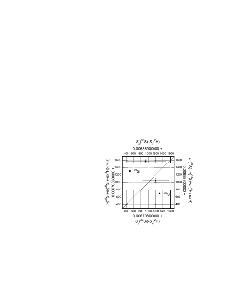
Figure 4: Mass differences determined in a Penning trap versus those determined from wavelength determinations. The left (right) and bottom (top) axes correspond to Si (S). The scales of the axes have been chosen so that a diagonal line through the plot represents exact consistency between Penning trap and gamma-ray measurements. The plot shows that the quality of the consistency test is limited by the uncertainty of the gamma-ray measurements.