ELECTROMAGNETIC FORM FACTORS OF THE NUCLEON AND COMPTON SCATTERING

Abstract

We review the experimental and theoretical status of elastic electron scattering and elastic low-energy photon scattering (with both real and virtual photons) from the nucleon. As a consequence of new experimental facilities and new theoretical insights, these subjects are advancing with unprecedented precision. These reactions provide many important insights into the spatial distributions and correlations of quarks in the nucleon.

1 General Introduction

Although nucleons account for nearly all the visible mass in the universe, they have a complicated structure that is still incompletely understood. The first indication that nucleons have an internal structure, was the 1933 measurement of the proton magnetic moment by Frisch & Stern[1]. The investigation of the spatial structure of the nucleon was initiated by the HEPL (Stanford) experiments in the 1950s, for which Hofstadter was awarded the 1961 Nobel prize. Several volumes of the Annual Review of Nuclear Science[2, 3] reviewed the status of this field. The recent revival of its experimental study through the operational implementation of novel instrumentation has instigated a strong theoretical interest.

Nucleon electro-magnetic form factors (EMFFs) are optimally studied through the exchange of a virtual photon, in elastic electron-nucleon scattering. The momentum transfer to the nucleon can be selected to probe different scales of the nucleon, from integral properties such as the charge radius to scaling properties of its internal constituents. Polarization instrumentation, polarized beams and targets, and the measurement of the recoil polarization have been essential in the accurate separation of the charge and magnetic form factors and in studies of the elusive neutron charge form factor.

Exclusive Compton scattering on a nucleon refers to the reactions $\gamma N\rightarrow\gamma^{\prime}N^{\prime}$, where either photon may be real or virtual. In general, the Compton amplitude depends on the full complexity of the dynamics of the excitation spectrum of the nucleon. However, in a number of special kinematic domains, observables with a particularly simple interpretation can be extracted from the Compton amplitude. In this review, we present the experimental and theoretical status of real (RCS) and virtual (VCS) Compton scattering for the study of generalized polarizabilities, which measure the spatial distribution of the response of the nucleon to external electromagnetic fields. A thorough discussion of the rapid developments in high energy Compton scattering, in both the deep virtual and hard scattering limits, is beyond the scope of this review.

2 Nucleon Form Factors

2.1 Theory of Electron Scattering and Form Factor Measurements

The nucleon EMFFs are of fundamental importance for the understanding of the nucleon’s internal structure. Under Lorentz invariance, spatial symmetries, and charge conservation, the most general form of the electromagnetic current inside a nucleon can be written as:

$$J_{EM}^{\mu}=F_{1}(Q^{2})\gamma^{\mu}+\frac{\kappa}{2M_{N}}F_{2}(Q^{2})i\sigma^{\mu\nu}q_{\nu},$$ (1)

where $F_{1}$ denotes the helicity non-flip Dirac form factor, $F_{2}$ the helicity flip Pauli form factor, $Q^{2}=-q^{2}$, and $\kappa$ the nucleon anomalous magnetic moment. The remaining variables are defined in Figure 1. The second term, usually referred to as the Foldy contribution, is of relativistic origin. It is useful to introduce the isospin form-factor components, corresponding to the isoscalar ($s$) and isovector ($v$) response of the nucleon,

$$F_{i}^{s}=\frac{1}{2}(F_{i}^{p}+F_{i}^{n});~{}~{}~{}~{}~{}F_{i}^{v}=\frac{1}{2}(F_{i}^{p}-F_{i}^{n});~{}~{}~{}~{}~{}(i=1,2).$$ (2)

Figure 1: The Feynman diagram for the scattering of an electron with four-momentum $p=(E_{e},\vec{p})$ through an angle $\theta_{e}$ off a nucleon with mass $M_{N}$ and four-momentum $P$. In this diagram a single virtual photon with four-momentum $q=p-p^{\prime}=(\omega,\vec{q})$ is exchanged. The four-momenta of the scattered electron and nucleon are $p^{\prime}=(E^{\prime}_{e},\vec{p^{\prime}})$ and $P^{\prime}$, respectively.

The form factors can be continued analytically into the complex plane and can be related in different regions through a dispersion relation of the form

$$F(t)=\frac{1}{\pi}\int^{\infty}_{t_{0}}\frac{\Im F(t^{\prime})}{t^{\prime}-t}dt^{\prime},$$ (3)

with $t=-Q^{2}$, $t_{0}=9(4)M_{\pi}^{2}$ for the isoscalar (isovector) case and $M_{\pi}$ the pion mass. In the positive $Q^{2}{}$-region, called spacelike, form factors can be measured through electron scattering, in the negative $Q^{2}{}$-region, called timelike, form factors can only be measured through the creation or annihilation of a $N\bar{N}$-pair.

In plane-wave Born approximation, the cross section for elastic electron-nucleon scattering can be expressed in the Rosenbluth[4] formula as:

$$\frac{d\sigma}{d\Omega}=\sigma_{M}[(F_{1}^{2}+\kappa^{2}\tau F_{2}^{2})+2\tau(F_{1}+\kappa F_{2})^{2}\tan^{2}(\frac{\theta_{e}}{2})],$$ (4)

where $\tau=Q^{2}/(4M_{N}^{2})$ and $\sigma_{M}=(\frac{\alpha_{QED}\cos\theta_{e}/2}{2E_{e}\sin^{2}\theta_{e}/2})^{2}\frac{E_{e}^{\prime}}{E_{e}}$ is the Mott cross section for scattering off a point-like particle, with $\alpha_{QED}$ denoting the fine-structure constant. The remaining variables are defined in Figure 1. Hofstadter[5] determined the values of $F_{1}$ and $F_{2}$ from measurements at different scattering angles but at the same values of $Q^{2}$ by drawing intersecting ellipses. Hand, Miller and Wilson[6] pointed out that a simple algebraic separation is possible if one expresses the Rosenbuth formula in an alternate form:

$$\frac{d\sigma}{d\Omega}=\sigma_{M}[\frac{(G^{p}_{E})^{2}+\tau(G^{p}_{M})^{2}}{1+\tau}+2\tau(G^{p}_{M})^{2}\tan^{2}(\frac{\theta_{e}}{2})]=\frac{\sigma_{M}}{\epsilon}[\tau(G^{p}_{M})^{2}+\epsilon(G^{p}_{E})^{2}](\frac{1}{1+\tau}),$$ (5)

with $\epsilon=1/[1+2(1+\tau)\tan^{2}(\frac{\theta_{e}}{2})]$ the linear polarization of the virtual photon. They further noted that $G_{E}$ and $G_{M}$ were identical to the electric and magnetic form factors, discussed earlier by Ernst, Sachs and Wali[7]:

$$G_{E}(Q^{2})=F_{1}(Q^{2})-\tau\kappa F_{2}(Q^{2}); G_{E}^{p}(0)=1; G_{E}^{n}(0)=0;$$

$$G_{M}(Q^{2})=F_{1}(Q^{2})+\kappa F_{2}(Q^{2}); G_{M}^{p,n}(0)=\mu_{p,n},$$ (6)

with $\mu_{p,n}$ denoting the magnetic moment of the proton and neutron, respectively. Equation 5 illustrates that $G_{E}^{p}$ and $G_{M}^{p}$ can be determined separately by performing cross-section measurements at fixed $Q^{2}{}$ as a function of $\epsilon$, over a range of ($\theta_{e}$,$E_{e}$) combinations (Rosenbluth separation). Hand, Miller and Wilson further noted that in the Breit frame, which for elastic scattering is equivalent to the centre-of-mass frame, the electromagnetic current of the proton simplifies into the expression:

$$J_{EM}^{\mu}=G_{E}(Q^{2})\gamma^{\mu}+G_{M}(Q^{2})i\sigma^{\mu\nu}q_{\nu}.$$ (7)

In this reference frame the Sachs form factors can be identified with the Fourier transform of the nucleon charge and magnetization density distributions.

Through the mid-1990s practically all available proton EMFF data had been collected using the Rosenbluth separation technique. This experimental procedure requires an accurate knowledge of the electron energy and the total luminosity. In addition, because the $G_{M}^{p}$ contribution to the elastic cross section is weighted with $Q^{2}{}$, data on $G_{E}^{p}$ suffer from increasing systematic uncertainties with increasing $Q^{2}{}$-values. The then available world data set[8] was compared to the so-called dipole parametrization $G_{D}$, which corresponds to two poles with opposite sign close to each other in the time-like region. In coordinate space $G_{D}$ corresponds to exponentially decreasing radial charge and magnetization densities, albeit with a non-physical discontinuity at the origin:

$$G_{D}=\left(\frac{\Lambda^{2}}{\Lambda^{2}+Q^{2}}\right)^{2}\mbox{~{}~{}~{}~{}~{}with $\Lambda$ = 0.84~{}GeV and $Q$ in GeV}.$$ (8)

For $G_{E}^{p}$, $G_{M}^{p}/\mu_{p}$ and $G_{M}^{n}{}/\mu_{n}$ the available data agreed to within 20% with the dipole parametrization. Both the $G_{E}^{p}$ and the $G_{M}^{p}/\mu_{p}$ data could be fitted adequately with an identical parametrization. However, the limitation of the Rosenbluth separation was evident from the fact that different data sets for $\mu_{p}G_{E}^{p}/G_{M}^{p}$ scattered by up to 50% at $Q^{2}{}$-values larger than 1 GeV² (Figure 2). Although no fundamental reason has been found for the success of the dipole parametrization, it is still used as a base line for comparison of data because it takes out the largest variation with $Q^{2}$ and enables smaller differences to be seen.

Figure 2: The ratio $\mu_{p}G_{E}^{p}/G_{M}^{p}$ from Rosenbluth separation. Data are from References [9, 10, 11, 12, 13, 14]. The errors shown are the quadratic sum of the statistical and systematic contributions.

2.2 Instrumentation for Form Factor Measurements

More than 40 years ago Akhiezer et al.[15] (followed 20 years later by Arnold et al.[16]) showed that the accuracy of nucleon charge form-factor measurements could be increased significantly by scattering polarized electrons off a polarized target (or equivalently by measuring the polarization of the recoiling proton). However, it took several decades before technology had sufficiently advanced to make the first of such measurements feasible, and only in the past few years has a large number of new data with a significantly improved accuracy become available. The next few sections introduce the various techniques. For $G_{E}^{p}$ measurements, the highest figure of merit at $Q^{2}{}$-values larger than a few GeV² is obtained with a focal plane polarimeter. Here, the Jacobian focusing of the recoiling proton kinematics allows one to couple a standard magnetic spectrometer for the proton detection to a large-acceptance non-magnetic detector for the detection of the scattered electron. For studies of $G_{E}^{n}$  one needs to use a magnetic spectrometer to detect the scattered electron in order to cleanly identify the reaction channel. As a consequence, the figure of merit of a polarized $\stackrel{{\scriptstyle\rightarrow}}{{{}^{3}\rm{He}}}$ target is comparable to that of a neutron polarimeter.

2.2.1 Polarized Beam

Various techniques are available to produce polarized electron beams, but photo-emission from GaAs has until now proven to be optimal[17]. A thin layer of GaAs is illuminated by a circularly polarized laser beam of high intensity, which preferentially excites electrons of one helicity state to the conductance band through optical pumping. The helicity sign of the laser beam can be flipped at a rate of tens of Hertz by changing the high voltage on a Pockels cell. The polarized electrons that diffuse to the photocathode surface are then extracted by a 50-100 kV potential. An ultra-high vacuum environment is required to minimize surface degradation of the GaAs crystal by backstreaming ions. Initially, the use of bulk GaAs limited the maximum polarization to 50% because of the degeneracy of the $P_{3/2}$ sublevels. This degeneracy is removed by introducing a strain in a thin layer of GaAs deposited onto a thicker layer with a slightly different lattice spacing. Although such strained GaAs cathodes have a significantly lower quantum efficiency than bulk GaAs cathodes, this has been compensated by the development of high-intensity diode or Ti-sapphire lasers. Polarized electron beams are now reliably available with a polarization close to 80% at currents of $\geq 100~{}\mu$A.

The polarized electrons extracted from the GaAs surface are first pre-accelerated and longitudinally bunched and then injected into an accelerator. Typically, the polarization vector of the electrons is manipulated in a Wien filter so that the electrons are fully longitudinally polarized at the target. If the beam is injected into a storage ring for use with an internal target, a Siberian snake[18] is needed to compensate for the precession of the polarization.

Three processes are used to measure the beam polarization: Mott[19] scattering, Møller[20] scattering or Compton[21] scattering. Any of these results in a polarimeter with an accuracy approaching 1%. In a Mott polarimeter the beam helicity asymmetry is measured in scattering polarized electrons off atomic nuclei. This technique is limited to electron energies below $\sim 20$ MeV and multiple scattering effects have to be estimated by taking measurements at different target foil thicknesses. In a Møller polarimeter polarized electrons are scattered off polarized atomic electrons in a magnetized iron foil. In this technique the major uncertainties are in the corrections for atomic screening and in the foil magnetization, unless the polarizing field is strong enough to saturate the magnetization. A potentially superior alternative[22] has been proposed in which the electrons are scattered off a sample of atomic hydrogen, polarized to a very high degree in an atomic beam, and trapped in a superconducting solenoid. Finally, in a Compton polarimeter the beam helicity asymmetry is measured in scattering polarized electrons off an intense beam of circularly polarized light, produced by trapping a laser beam in a high-finesse Fabry-Perot cavity. The electron beam in a storage ring is sufficiently intense that a laser beam can be directly scattered off the electron beam without the use of an amplifying cavity. Only the last two methods, the atomic hydrogen Møller and the Compton polarimeter, have no effect on the quality of the electron beam and thus can be used continuously during an experiment.

2.2.2 Polarized Targets

In polarized targets for protons two different techniques are used, depending on the intensity of the electron beam. In storage rings where the circulating beam can have an intensity of 100 mA or more, but the material interfering with the beam has to be minimized, gaseous targets are used, whereas in external targets solid targets can be used. Because free neutrons are not available in sufficient quantity, effective targets, such as deuterium or ³He, are necessary, and the techniques used to polarize the deuteron are similar to those used for the proton. For ³He gaseous targets are used both in internal and external targets.

Solid polarized targets that can withstand electron beams with an intensity of up to 100 nA all use the dynamic nuclear polarization technique[23]. A hydrogenous compound, such as NH₃ or LiD, is doped, e.g. by radiation damage, with a small concentration of free radicals. Because the occupation of the magnetic substates in the radicals follows the Boltzmann distribution, the free electrons are polarized to more than 99% in a $\sim 5$ T magnetic field and at a $\sim 1$ K temperature. A radiofrequency (RF) field is then applied to induce transitions to states with a preferred orientation of the nuclear spin. Because the relaxation time of the electrons is much shorter than that of the nuclei, polarized nuclei are accumulated. This technique has been successful in numerous deep-inelastic lepton scattering and nucleon form-factor experiments; it has provided polarized hydrogen or deuterium targets with an average polarization of $\sim 80$% or $\sim 30$%, respectively.

Internal hydrogen/deuterium targets[24] are polarized by the atomic beam source (ABS) technique, which relies on Stern-Gerlach separation and RF transitions. First, a beam of atoms is produced in an RF dissociator through a nozzle cooled with liquid nitrogen. Then, atoms with different electron spin direction are separated through a series of permanent (or superconducting) sextupole magnets and transitions between different hyperfine states are induced by a variety of RF units. The result is a highly polarized beam with a flux up to $10^{17}$ atoms/s. This beam is then fed into an open-ended storage cell, which is cooled and coated to minimize recombination of the atoms bouncing off the cell walls. The circulating electron beam, passing through the long axis of the storage cell, encounters only the flowing atoms. The polarization vector is oriented with a set of coils, producing a field of $\sim 0.3$ T in order to minimize depolarization by the RF structure of the circulating electron beam. The diameter of the storage cell is determined by the halo of the electron beam. A target thickness of $2\times 10^{14}$ nuclei/cm² has been obtained at a vector polarization of more than 80%.

Polarized hydrogen or deuterium atoms can also be produced by spin-exchange collisions between such atoms and a small admixture of alkali atoms that have been polarized by optical pumping. The nucleus is then polarized in spin-temperature equilibrium. Although the nuclear polarization obtained in such a laser driven source (LDS) is smaller than through the ABS technique, the flux can be more than $10^{18}$ atoms/s. Moreover, an LDS offers a more compact design than an ABS. A figure of merit comparable to that of the ABS at the HERMES experiment has recently been achieved by the MIT group[25].

Polarized ³He is attractive as an effective polarized neutron target because its ground state is dominated by a spatially symmetric $s$-state in which the proton spins cancel, so that the spin of the ³He nucleus is mainly determined by that of the neutron. Corrections for the (small) $d$-state component and for charge-exchange contributions from the protons can be calculated accurately at $Q^{2}{}$-values smaller than 0.5 GeV²[26] and larger than $\sim 2$ GeV²[27]. Direct optical pumping of ³He atoms is not possible because of the energy difference between the ground state and the first excited state. Instead ³He is polarized, either by first exciting the atoms to a metastable $2^{3}S_{1}$ state and optically pumping that state, which then transfers its polarization to the ground state by metastability-exchange collisions, or by optically pumping a small admixture of rubidium atoms, which then transfer their polarization to the ³He atoms through spin-exchange collisions. In internal targets only the metastability-exchange technique has been used because of the possible detrimental effects of the rubidium admixture on the storage ring environment. With beam on target, polarization values of up to 46% at target thicknesses of $1\times 10^{15}$ nuclei/cm² have been obtained. For external targets the spin-exchange technique[28] has been used to optically pump a glass target cell filled with 10 atm of ³He with a 0.1% rubidium admixture. After the spin-exchange collisions the polarized ³He diffuses into a 25 cm long cell which the electron beam traverses. Polarizations in excess of 40% have been reached with beam on target. A pair of 5 mT Helmholz coils is used to orient the polarization vector, and care must be taken to minimize depolarizing magnetic field gradients. Alternatively, the metastability technique[29] has been used to polarize ³He under atmospheric pressure which is then compressed to a density of more than 6 atm.

2.2.3 Recoil Polarimeters

Focal-plane polarimeters have long been used at proton scattering facilities to measure the polarization of the scattered proton. In such an instrument[28] the azimuthal angular distribution is measured of protons scattered in the focal plane of a magnetic spectrometer by an analyzer, which often consists of carbon. From this angular distribution the two polarization components transverse to the proton momentum can be derived. The analyzer is preceded by two detectors, most often wire or straw chambers, to measure the track of the incident proton; it is followed by two more detectors to track the scattered particle. The thickness of the analyzer is adjusted to the proton momentum, limiting multiple scattering while optimizing the figure of merit. In order to determine the two polarization components in the scattering plane at the target, care must be taken to accurately calculate on an event-by-event basis the precession of the proton spin in the magnetic field of the spectrometer.

Neutron polarimeters follow the same basic principle. Here, plastic scintillator material is used as an active analyzer, preceded by a veto counter to discard charged particles. This eliminates the need for the front detectors. Sets of scintillator detectors are used to measure an up-down asymmetry in the scattered neutrons, which is sensitive to a polarization component in the scattering plane, perpendicular to the neutron momentum. In modern neutron polarimeters[30] the analyzer is preceded by a dipole magnet, with which the neutron spin can be precessed.

2.3 Experimental Results

2.3.1 Proton Electric Form Factor

In elastic electron-proton scattering a longitudinally polarized electron will transfer its polarization to the recoil proton. In the one-photon exchange approximation the proton can attain only polarization components in the scattering plane, parallel ($P_{l}$) and transverse ($P_{t}$) to its momentum. This can be immediately seen from the expression for the proton current in the Breit frame, which separates into components proportional to $G_{E}$ and $G_{M}$ to which reference was made in eq. 7. The ratio of the charge and magnetic form factors is directly proportional to the ratio of these polarization components[31]:

$$\frac{G_{E}^{p}}{G_{M}^{p}}=-\frac{P_{t}}{P_{l}}\frac{E_{e}+E_{e}^{\prime}}{2M}\tan(\frac{\theta_{e}}{2}).$$ (9)

The polarization-transfer technique was used for the first time by Milbrath et al.[32] at the MIT-Bates facility. The proton form factor ratio was measured at $Q^{2}{}$-values of 0.38 and 0.50 GeV² by scattering a 580 MeV electron beam polarized to $\sim 30$%. A follow-up measurement was performed at the MAMI facility[33] at a $Q^{2}{}$-value of 0.4 GeV².

Figure 3: The ratio $\mu_{p}G_{E}^{p}/G_{M}^{p}$ from polarization transfer[32, 33, 34, 36, 35], compared to recent Rosenbluth data[39, 37] and the reanalysis by Arrington[38] of older SLAC data.

The greatest impact of the polarization-transfer technique was made by the two recent experiments[34, 35] in Hall A at Jefferson Lab, which measured the ratio $G_{E}^{p}/G_{M}^{p}$ in a $Q^{2}{}$-range from 0.5 to 5.6 GeV². Elastic $ep$ events were selected by detecting electrons and protons in coincidence in the two identical high-resolution spectrometers. At the four highest $Q^{2}{}$-values a lead-glass calorimeter was used to detect the scattered electrons in order to match the proton angular acceptance. The polarization of the recoiling proton was determined with a focal-plane polarimeter in the hadron spectrometer, consisting of two pairs of straw chambers with a carbon or polyethylene analyzer in between. The data were analyzed in bins of each of the target coordinates. No dependence on any of these variables was observed[34]. Figure 3 shows the results for the ratio $\mu_{p}G_{E}^{p}/G_{M}^{p}$ . The most striking feature of the data is the sharp, practically linear decline as $Q^{2}{}$ increases:

$$\mu_{p}\frac{G_{E}^{p}(Q^{2}{})}{G_{M}^{p}(Q^{2}{})}=1-0.13(Q^{2}{}-0.29\rm{GeV^{2}}).$$ (10)

Since it is known that $G_{M}^{p}$ closely follows the dipole parametrization, it follows that $G_{E}^{p}$ falls more rapidly with $Q^{2}{}$ than $G_{D}$. This significant fall-off of the form-factor ratio is in clear disagreement with the results from the Rosenbluth extraction. Arrington[38] has performed a careful reanalysis of earlier Rosenbluth data. He selected only experiments in which an adequate $\epsilon$-range was covered with the same detector. The results (Figure 3) do not show the large scatter seen in Figure 2. Recently, Christy et al.[37] analyzed an extensive data set on elastic electron-proton scattering collected in Hall C at Jefferson Lab as part of experiment E99-119. The results are evidently in good agreement with Arrington’s reanalysis. Qattan et al. [39] performed a high-precision Rosenbluth extraction in Hall A at Jefferson Lab, designed specifically to significantly reduce the systematic errors compared to earlier Rosenbluth measurements. The main improvement came from detecting the recoiling protons instead of the scattered electrons, so that the proton momentum and the cross section remain practically constant when one varies $\epsilon$ at a constant $Q^{2}{}$-value. In addition, possible dependences on the beam current are minimized. Special care was taken in surveying the angular setting of the identical spectrometer pair. One of the spectrometers was used as a luminosity monitor during an $\epsilon$ scan. The results[39] of this experiment, covering $Q^{2}{}$-values from 2.6 to 4.1 GeV², are in excellent agreement with previous Rosenbluth results. This basically rules out the possibility that the disagreement between Rosenbluth and polarization-transfer measurements of the ratio $G_{E}^{p}/G_{M}^{p}$ is due to an underestimate of $\epsilon$-dependent uncertainties in the Rosenbluth measurements.

2.3.2 Two-Photon Exchange

In order to resolve the discrepancy between the results for $G_{E}^{p}/G_{M}^{p}$ from the two experimental techniques, an $\epsilon$-dependent modification of the cross section is necessary. In two-(or more-)photon exchanges (TPE) the nucleon undergoes a first virtual photon exchange which can lead to an intermediate excited state and then a second one or more, finally ending back in its ground state (Figure 4). The TPE contributions to elastic electron scattering have been investigated both experimentally and theoretically for the past fifty years. In the early days such contributions were called dispersive effects[40]. Lately, they have been relocated to radiative corrections in the so-called box diagram. Almost all analyses with the Rosenbluth technique have applied radiative corrections using the formulae derived by Mo & Tsai[41] that only include the infrared divergent parts of the box diagram (in which one of the two exchanged photons is soft). Thus, terms in which both photons are hard (and which depend on the hadronic structure) have been ignored.

Figure 4: The Feynman diagrams depicting two-photon exchanges.

The most stringent tests of TPE on the nucleon have been carried out by measuring the ratio of electron and positron elastic scattering off a proton. Corrections due to TPE will have a different sign in these two reactions. Unfortunately, this (e⁺e^-) data set is quite limited[44], only extending (with poor statistics) up to a $Q^{2}{}$-value of $\sim 5$ GeV², whereas at $Q^{2}{}$-values larger than $\sim 2$ GeV² basically all data have been measured at $\epsilon$-values larger than $\sim 0.85$. Other tests, also inconclusive, searched for non-linearities in the $\epsilon$-dependence or measured the transverse (out-of-plane) polarization component of the recoiling proton, of which a non-zero value would be a direct measure of the imaginary part of the TPE amplitude.

Several studies have provided estimates of the size of the $\epsilon$-dependent corrections necessary to resolve the discrepancy. Because the fall-off of the form-factor ratio is linear with $Q^{2}{}$, and the Rosenbluth formula also shows a linear dependence of the form-factor ratio (squared) with $Q^{2}{}$ through the $\tau$-term, a $Q^{2}{}$-independent correction linear in $\epsilon$ would cancel the disagreement. An additional constraint that any $\epsilon$-dependent modification must satisfy, is the (e⁺e^-) data set. Guichon & Vanderhaeghen[42] introduced a general form of a TPE contribution from the so-called box diagram in radiative corrections into the amplitude for elastic electron-proton scattering. This resulted in the following modification of the Rosenbluth expression:

$$d\sigma\propto{\tau+\epsilon\frac{\tilde{G_{E}}^{2}}{\tilde{G_{M}}^{2}}+2\epsilon(\tau+\frac{\tilde{G_{E}}}{\tilde{G_{M}}})Y_{2\gamma}},$$ (11)

where $Y_{2\gamma}=\Re{\frac{\nu\tilde{F_{3}}}{M^{2}\tilde{G_{M}}}}$ and $\tilde{G_{M}}$, $\tilde{F_{2}}$ and $\tilde{F_{3}}$ are equal to $G_{M}$, $F_{2}$ and 0, respectively, in the Born approximation. $Y_{2\gamma}$ and the ”two-photon” form factors $\tilde{G_{E}}$ and $\tilde{G_{M}}$ were fitted[42] to the Rosenbluth and polarization transfer data sets. This resulted in a value of $\sim$ 0.03 for $Y_{2\gamma}$ with very little $\epsilon$- or $Q^{2}{}$-dependence.

Arrington[43] performed a fit to the complete data set, investigating two different modifications to the cross section with a $Q^{2}{}$-independent linear $\epsilon$-dependence of 6 % over the full $\epsilon$-range. Both modifications have the same $\epsilon$-dependence, but one does not modify the cross section at small values of $\epsilon$, whereas the other leaves the cross section unchanged at large values of $\epsilon$. He found that the second gave a much better description of the complete data set. Moreover, it was in good agreement with the data set for the ratio of electron-proton and positron-proton elastic scattering.

Blunden et al.[45] carried out the first calculation of the elastic contribution from TPE effects, albeit with a simple monopole $Q^{2}{}$-dependence of the hadronic form factors: $G(Q^{2})=\Lambda^{2}/(Q^{2}+\Lambda^{2})$. They obtained a practically $Q^{2}{}$-independent correction factor with a linear $\epsilon$-dependence that vanishes at forward angles ($\epsilon=1$). However, the size of the correction only resolves about half of the discrepancy. A later calculation(W. Melnitchouk, private communication) which used a more realistic form factor behavior, resolved up to 80% of the discrepancy.

A different approach was used by Chen et al.[46], who related the elastic electron-nucleon scattering to the scattering off a parton in a nucleon through generalized parton distributions. TPE effects in the lepton-quark scattering process are calculated in the hard-scattering amplitudes. The handbag formalism of the generalized parton distributions is extended in an unfactorized framework in which the $x$-dependence is retained in the scattering amplitude. Finally, a valence model is used for the generalized parton distributions. The results for the TPE contribution fully reconcile the Rosenbluth and the polarization-transfer data and retain agreement with positron-scattering data.

Hence, it is becoming more and more likely that TPE processes have to be taken into account in the analysis of Rosenbluth data and that they will affect polarization-transfer data only at the few percent level. Of course, further effort is needed to investigate the model-dependence of the TPE calculations. Experimental confirmation of TPE effects will be difficult, but certainly should be continued. The most direct test would be a measurement of the positron-proton and electron-proton scattering cross-section ratio at small $\epsilon$-values and $Q^{2}{}$-values above 2 GeV². Positron beams available at storage rings are too low in either energy or intensity, but a measurement in the CLAS detector at Jefferson Lab, a more promising venue, has been proposed[47]. A measurement of the beam or target single-spin asymmetry normal to the scattering plane, which directly accesses the imaginary part of the box diagrams, would provide a sensitive test of TPE calculations. Also, real and virtual Compton scattering data can provide additional constraints on calculations of TPE effects in elastic scattering. Rosenbluth analyses have so far been restricted to simple PWBA, Coulomb distortion effects should certainly be included too. Additional efforts should be extended to studies of TPE effects in other longitudinal-transverse separations, such as proton knock-out and deep-inelastic scattering (DIS) experiments.

2.3.3 Proton Magnetic Form Factor

An extensive data set[48] with a good accuracy is available up to a $Q^{2}{}$-value of more than 30 GeV² from unpolarized cross-section measurements (Figure 5). Because $G_{M}^{p}$ dominates in a Rosenbluth extraction at larger $Q^{2}{}$-values, the $G_{M}^{p}$ data have only a minor sensitivity to the discrepancy between the Rosenbluth extraction and the polarization-transfer technique. Brash et al.[51] have shown that the $G_{M}^{p}$ data must be renormalized upwards by $\sim$ 2% if one assumes the polarization-transfer data to be correct.

Figure 5: The proton magnetic form factor $G_{M}^{p}$, in units of $\mu_{p}G_{D}$, as a function of $Q^{2}{}$. Data are from References [48, 49, 50, 13, 14].

2.3.4 Neutron Magnetic Form Factor

Early data on $G_{M}^{n}{}$ were extracted from inclusive quasi-elastic scattering off the deuteron. However, modeling of the deuteron wave function, required to subtract the contribution from the proton, resulted in sizable systematic uncertainties. A significant break-through was made by measuring the ratio of quasi-elastic neutron and proton knock-out from a deuterium target. This method has little sensitivity to nuclear binding effects and to fluctuations in the luminosity and detector acceptance. The basic set-up used in all such measurements is very similar: the electron is detected in a magnetic spectrometer with coincident neutron/proton detection in a large scintillator array. The main technical difficulty in such a ratio measurement is the absolute determination of the neutron detection efficiency. Such measurements have been pioneered for $Q^{2}{}$-values smaller than 1 GeV² at Mainz[53, 54, 55] and Bonn[56]. The Mainz $G_{M}^{n}{}$ data are 8%-10% lower than those from Bonn, at variance with the quoted uncertainty of $\sim$2%. This discrepancy would require a 16%-20% error in the detector efficiency.

A study of $G_{M}^{n}{}$ at $Q^{2}{}$-values up to 5 GeV² has recently been completed in Hall B by measuring the neutron/proton quasi-elastic cross-section ratio using the CLAS detector[57]. A hydrogen target was in the beam simultaneously with the deuterium target. This made it possible to measure the neutron detection efficiency by tagging neutrons in exclusive reactions on the hydrogen target. Preliminary results[57] indicate that $G_{M}^{n}{}$ is within 10% of $G_{D}$ over the full $Q^{2}{}$-range of the experiment (0.5-4.8 GeV²).

Inclusive quasi-elastic scattering of polarized electrons off a polarized ³He target offers an alternative method to determine $G_{M}^{n}{}$ through a measurement of the beam asymmetry[58]

$$A=-\frac{(\cos\theta^{*}v_{T^{\prime}}R_{T^{\prime}}+2\sin\theta^{*}\cos\theta^{*}v_{TL^{\prime}}R_{TL^{\prime}})}{v_{L}R_{L}+v_{T}R_{T}},$$ (12)

where $\theta^{*}$ and $\phi^{*}$ are the polar and azimuthal target spin angles with respect to $\vec{q}$, $R_{i}$ denote various nucleon response functions, and $v_{i}$ the corresponding kinematic factors. By orienting the target polarization parallel to $\vec{q}$, one measure $R_{T\prime}$, which in quasi-elastic kinematics is dominantly sensitive to $(G_{M}^{n}{})^{2}$. For the extraction of $G_{M}^{n}{}$ corrections for the nuclear medium[26] are necessary to take into account effects of final-state interactions and meson-exchange currents. The first such measurement was carried out at Bates[59]. Recently, this technique was used to measure $G_{M}^{n}{}$ in Hall A at Jefferson Lab in a $Q^{2}{}$-range from 0.1 to 0.6 GeV²[60]. This experiment provided an independent, accurate measurement of $G_{M}^{n}{}$ at $Q^{2}{}$-values of 0.1 and 0.2 GeV², in excellent agreement with the Mainz data. At the higher $Q^{2}{}$-values $G_{M}^{n}{}$ could be extracted[61] in plane wave impulse approximation, since final-state interaction effects are expected to decrease with increasing $Q^{2}{}$.

Figure 6: The neutron magnetic form factor $G_{M}^{n}{}$, in units of $\mu_{n}G_{D}$, as a function of $Q^{2}{}$. Results from $\stackrel{{\scriptstyle\rightarrow}}{{{}^{3}\rm{He}}}$ are indicated by open symbols. Data are from References [62, 52, 63, 64, 53, 56, 54, 55, 59, 60, 61].

Figure 6 shows the results of all completed $G_{M}^{n}{}$ experiments.

2.3.5 Neutron Electric Form Factor

Analogously to $G_{M}^{n}{}$, early $G_{E}^{n}$-experiments used (quasi-)elastic scattering off the deuteron to extract the longitudinal deuteron response function. Due to the smallness of $G_{E}^{n}$, the use of different nucleon-nucleon potentials resulted in a 100% spread in the resulting $G_{E}^{n}$ values[65]. In the past decade a series of double-polarization measurements of neutron knock-out from a polarized ²H or ³He target have provided accurate data on $G_{E}^{n}$. The ratio of the beam-target asymmetry with the target polarization perpendicular and parallel to the momentum transfer is directly proportional to the ratio of the electric and magnetic form factors,

$$\frac{G_{E}^{n}}{G_{M}^{n}{}}=-\frac{P_{x}}{P_{z}}\frac{E_{e}+E_{e}^{\prime}}{2M}\tan(\frac{\theta_{e}}{2}),$$ (13)

where $P_{x}$ and $P_{z}$ denote the polarization component perpendicular and parallel to $\vec{q}$. A similar result is obtained with an unpolarized deuteron target when one measures the polarization of the knocked-out neutron as a function of the angle over which the neutron spin is precessed with a dipole magnet:

$$\frac{G_{E}^{n}}{G_{M}^{n}{}}=-\tan(\delta)\sqrt{\frac{\tau(1+\epsilon)}{2\epsilon}};$$ (14)

here, $\delta$ denotes the precession angle where the measured asymmetry is zero.

Figure 7: The neutron electric form factor $G_{E}^{n}$ as a function of $Q^{2}{}$. Results from $\stackrel{{\scriptstyle\rightarrow}}{{{}^{3}\rm{He}}}$ are indicated by open symbols. Data are from References [66, 67, 68, 30, 69, 70, 71, 72, 73, 26, 74]. The full curve shows the Galster[76] parametrization; the dashed curve represents the $Q^{2}{}$-behavior of $G_{E}^{p}$.

Again, the first such measurements were carried out at Bates, both with a polarized $\stackrel{{\scriptstyle\rightarrow}}{{{}^{3}\rm{He}}}$ target and with a neutron polarimeter. Figure 7 shows results obtained through all three reactions $\stackrel{{\scriptstyle\rightarrow}}{{{}^{2}\rm{H}}}$($\vec{e},e^{\prime}n$), ²H($\vec{e},e^{\prime}\vec{n})$ and $\stackrel{{\scriptstyle\rightarrow}}{{{}^{3}\rm{He}}}$($\vec{e},e^{\prime}n$). At low $Q^{2}{}$-values corrections for nuclear medium and rescattering effects can be sizeable: 65% for ²H at 0.15 GeV² and 50% for ${}^{3}\rm{He}$ at 0.35 GeV². These corrections are expected to decrease significantly with increasing $Q$, although no reliable calculations are presently available for ${}^{3}\rm{He}$ above 0.5 GeV². There is excellent agreement between the results from the different techniques. Moreover, medium effects have clearly become negligible at $\sim$ 0.7 GeV², even for ${}^{3}\rm{He}$. The latest data from Hall C at Jefferson Lab, using either a polarimeter or a polarized target [69, 71], extend up to $Q^{2}{}$ $\approx$ 1.5 GeV² with an overall accuracy of $\sim$10%, in mutual agreement. From $\sim$ 1 GeV² onwards $G_{E}^{n}$ appears to exhibit a $Q^{2}{}$-behavior similar to that of $G_{E}^{p}$. Schiavilla & Sick[75] have extracted $G_{E}^{n}$ from available data on the deuteron quadrupole form factor $F_{C2}(Q^{2})$ with a much smaller sensitivity to the nucleon-nucleon potential than from inclusive (quasi-)elastic scattering. The 30-years-old Galster parametrization[76] continues to provide a fortuitously good description of the data.

2.3.6 Timelike Form Factors

In the timelike region EMFF measurements have been made at electron-positron storage rings or by studying the inverse reaction (only for the proton form factors), antiproton annihilation on a hydrogen target. The rather limited data set on timelike form factors is shown in Figure 8. The quality of the data does not allow a separation of the charge and magnetic form factors; $G_{M}$ has been extracted from the data using the $G_{E}$-values calculated by Iachello & Wan[77]. Clearly $G_{D}$  which gives a very good description of the spacelike magnetic form factors, does not describe the data in the timelike region, at least from threshold down to -6 GeV². Iachello & Wan[77], Hammer et al.[78] and Dubnicka et al.[79] have carried out an analytic continuation of their VMD calculations (section 2.4). Iachello’s model provides a consistent description of the magnetic form factors in the timelike region. An extension of the data set in the timelike region and of theoretical efforts to obtain a consistent description of all EMFFs in both the space- and timelike regions is highly desirable.

Figure 8: The magnetic form factors (divided by $G_{D}$) in the time-like region as a function of $Q^{2}{}$, compared to the calculations by Iachello[77], Hammer[78] and Dubnicka[79]. See Reference [77] for the references to the experimental data.

2.3.7 Experimental Review and Outlook

In recent years highly accurate data on the nucleon EMFFs have become available from various facilities around the world, made possible by the development of high luminosity and novel polarization techniques. These have established some general trends in the $Q^{2}{}$-behavior of the four EMFFs. The two magnetic form factors $G_{M}^{p}$ and $G_{M}^{n}{}$ are close to identical, following $G_{D}$ to within 10% at least up to 5 GeV², with a shallow minimum at $\sim 0.25$ GeV² and crossing $G_{D}$ at $\sim 0.7$ GeV². $G_{E}^{p}/G_{M}^{p}$ drops linearly with $Q^{2}{}$  and $G_{E}^{n}$ appears to drop from $\sim 1$ GeV² onwards at the same rate as $G_{E}^{p}$. Measurements that extend to higher $Q^{2}{}$-values and offer improved accuracy at lower $Q^{2}{}$-values, will become available in the near future. In Hall C at Jefferson Lab Perdrisat et al.[80] will extend the measurements of $G_{E}^{p}/G_{M}^{p}$ to 9 GeV² with a new polarimeter and large-acceptance lead-glass calorimeter. Wojtsekhowski et al.[81] will measure $G_{E}^{n}$ in Hall A at $Q^{2}{}$-values of 2.4 and 3.4 GeV² using the $\stackrel{{\scriptstyle\rightarrow}}{{{}^{3}\rm{He}}}$($\vec{e},e^{\prime}n$) reaction with a 100 msr electron spectrometer. The Bates Large Acceptance Spectrometer Toroid facility (BLAST, http://www.mitbates.mit.edu) at MIT with a polarized hydrogen and deuteron target internal to a storage ring will provide highly accurate data on $G_{E}^{p}$ and $G_{E}^{n}$ in a $Q^{2}{}$-range from 0.1 to 0.8 GeV². Gao et al.[82] have shown that the proton charge radius can be measured with unprecedented precision by measuring the ratio of asymmetries in the two sectors of the BLAST detector. Thus, within a couple of years $G_{E}^{n}$ data with an accuracy of 10% or better will be available up to a $Q^{2}{}$-value of 3.4 GeV². Once the upgrade to 12 GeV[83] has been implemented at Jefferson Lab, it will be possible to extend the data set on $G_{E}^{p}$ and $G_{M}^{n}{}$ to 14 GeV² and on $G_{E}^{n}$ to 8 GeV².

The charge and magnetization rms radii are related to the slope of the form factor at $Q^{2}{}$= 0:

$$<r_{E}^{2}>=\int\rho(r)r^{4}dr=\left.-6\frac{dG(Q^{2})}{dQ^{2}}\right|_{Q^{2}=0}$$

$$<r_{M}^{2}>=\int\mu(r)r^{4}dr=\left.-\frac{6}{\mu}\frac{dG(Q^{2})}{dQ^{2}}\right|_{Q^{2}=0},$$ (15)

with $\rho$(r) ($\mu$(r)) denoting the radial charge (magnetization) distribution. Table 1 lists the results. For an accurate extraction of the radius Sick[84] has shown that it is necessary to take into account Coulomb distortion effects and higher moments of the radial distribution. His result for the proton charge radius is in excellent agreement with the most recent three-loop QED calculation[85] of the hydrogen Lamb shift. Within error bars the rms radii for the proton charge and magnetization distribution and for the neutron magnetization distribution are equal. The value for the neutron charge radius was obtained by measuring the transmission of low-energy neutrons through liquid ²⁰⁸Pb and ²⁰⁹Bi. The Foldy term $\frac{3}{2}\frac{\kappa}{M_{n}^{2}}=-0.126$ fm² is close to the value of the neutron charge radius. Isgur[87] showed that the Foldy term is canceled by a first-order relativistic correction, which implies that the measured value of the neutron charge radius is indeed dominated by its internal structure.

Table 1: Values for the nucleon charge and magnetization radii

Observable	value $\pm$ error	Reference
$<(r_{E}^{p})^{2}>^{1/2}$	0.895 $\pm$ 0.018 fm	[84]
$<(r_{M}^{p})^{2}>^{1/2}$	0.855 $\pm$ 0.035 fm	[84]
$<(r_{E}^{n})^{2}>$	- 0.119 $\pm$ 0.003 fm2	[86]
$<(r_{M}^{n})^{2}>^{1/2}$	0.87 $\pm$ 0.01 fm	[55]

In the Breit frame the nucleon form factors can be written as Fourier transforms of their charge and magnetization distributions. However, if the wavelength of the probe is larger than the Compton wavelength of the nucleon, i.e. if $|Q|\geq M_{N}$, the form factors are not solely determined by the internal structure of the nucleon. Then, they also contain dynamical effects due to relativistic boosts and consequently the physical interpretation of the form factors becomes complicated. Recently, Kelly[88] has extracted spatial nucleon densities from the available form factor data. He selected a model for the Lorentz contraction of the Breit frame in which the asymptotic behavior of the form factors conformed to perturbative quantum chromo-dynamics (pQCD) scaling at large $Q^{2}{}$-values and expanded the densities in a complete set of radial basis functions, with constraints at large radii. The neutron and proton magnetization densities are found to be quite similar, narrower than the proton charge density. He reports a neutron charge density with a positive core surrounded by a negative surface charge, peaking at just below 1 fm, which he attributes to a negative pion cloud. Alternatively, he extracts the radial distributions of the $u$ and $d$ quarks which both show a secondary lobe which he interprets as an indication of an orbital angular momentum (OAM) component in the quark distributions. Friedrich & Walcher[89] observe as a feature common to all EMFFs a bump/dip at $Q\approx$ 0.5 GeV with a width of $\sim$ 0.2 GeV. A fit to all four EMFFs was performed, assuming a dipole behaviour for the form factors of the constituent quarks and an $l=1$ harmonic oscillator behaviour for that of the pion cloud. They then transformed their results to coordinate space, neglecting the Lorentz boost, where they find that the pion cloud peaks at a radius of $\sim$ 1.3 fm, slightly larger than Kelly did, close to the Compton wavelength of the pion. Hammer et al.[90] argue from general principles that the pion cloud should peak much more inside the nucleon, at $\sim$ 0.3 fm. However, they assign the full $N\bar{N}$2$\pi$ continuum to the pion cloud which includes different contributions than just the one-pion loop that Kelly (and Friedrich & Walcher) assign to the pion cloud. The structure at $\sim$ 0.5 GeV, common to all EMFFs, is at such a small $Q^{2}{}$-value that its transformation to coordinate space should be straightforward.

2.4 Model Calculations

The recent production of very accurate EMFF data, especially the surprising $G_{E}^{p}$ data from polarization transfer, has prompted the theoretical community to intensify their investigation of nucleon structure. Space limitations compel us to focus on only a few highlights. The interested reader is encouraged to read the original publications; the review by Thomas & Weise[91] is an excellent introduction.

The $u$-, $d$- and $s$-quarks are the main building blocks of the nucleon in the kinematic domain relevant to this review. Its basic structure involves the three lightest vector mesons ($\rho$, $\omega$ and $\phi$) which have the same quantum numbers as the photon. Consequently, one should expect these vector mesons to play an important role in the interaction of the photon with a nucleon. The first EMFF models were based on this principle, called vector meson dominance (VMD), in which one assumes that the virtual photon - after becoming a quark-antiquark pair - couples to the nucleon as a vector meson. The EMFFs can then be expressed in terms of coupling strengths between the virtual photon and the vector meson and between the vector meson and the nucleon, summing over all possible vector mesons. In the scattering amplitude a bare-nucleon form factor is multiplied by the amplitude of the photon interaction with the vector meson. With this model Iachello et al.[92] predicted a linear drop of the proton form factor ratio, similar to that measured by polarization transfer, more than 20 years before the data became available. Gari & Krümpelmann[93] extended the VMD model to conform with pQCD scaling at large $Q^{2}{}$-values. The VMD picture is not complete, as becomes obvious from the fact that the Pauli isovector form factor $F_{2}^{V}$ is much larger than the isoscalar one $F_{2}^{S}$. An improved description requires the inclusion of the isovector $\pi\pi$ channel through dispersion relations[95, 96]. By adding more parameters, such as the width of the $\rho$-meson and the masses of heavier vector mesons[94], the VMD models succeeded in describing new EMFF data as they became available, but with little predictive power. Figure 9 confirms that Lomon’s calculations provide an excellent description of all EMFF data. Bijker & Iachello[97] have extended the original calculations by also including a meson-cloud contribution in $F_{2}$, but still taking only two isoscalar and one isovector poles into account. The intrinsic structure of the nucleon is estimated to have an rms radius of $\sim$ 0.34 fm. These new calculations are in good agreement with all EMFF data, except for $G_{M}^{n}$ at low $Q^{2}$-values. The most recent dispersion-theoretical analysis[78], using four isoscalar and three isovector mesons, results in an excellent description of $G_{M}^{p}$ and $G_{M}^{n}{}$, but only reasonably describes $G_{E}^{p}$ and $G_{E}^{n}$. Subsequent studies[98] have further developed this combined approach to include chiral perturbation theory. However, such models can only be used at small $Q^{2}{}$-values, $\leq 0.4$ GeV².

Figure 9: Comparison of various calculations with available EMFF data, indicated by the same symbols as in Figures 3, 5, 6 and 7. For $G_{E}^{p}$ only polarization-transfer data are shown. Not shown are the data for $G_{E}^{n}$ of References [72, 66] and the data for $G_{M}^{n}{}$ of References [52, 62, 64, 59, 56]. For $G_{E}^{n}$ the results of Schiavilla & Sick[75] have been added. The calculations shown are from References [97, 94, 78, 110, 111, 121]. Where applicable, the calculations have been normalized to the calculated values of $\mu_{p,n}$.

Many recent theoretical studies of the EMFFs have applied various forms of a relativistic constituent quark model (RCQM). Nucleons are assumed to be composed of three constituent quarks, which are quasi-particles where all degrees of freedom associated with the gluons and $q\bar{q}$ pairs are parametrized by an effective mass. Because the momentum transfer can be several times the nucleon mass, the constituent quarks require a relativistic quantum-mechanical treatment. Three possibilities exist for such a treatment: the instant form, where the interaction is present in the time component of the four-momentum and in the Lorentz boost; the point form, where all components of the four-momentum operator depend on the interaction; and the light-front form, where the interaction appears in one component of the four-momentum and in the transverse rotations. In each of these forms the Poincaré invariance can be broken in the number of constituents (by the creation of $q\bar{q}$ pairs) or by the use of approximate current operators. Although most of these calculations correctly describe the EMFF behaviour at large $Q^{2}{}$-values, effective degrees of freedom, such as a pion cloud and/or a finite size of the constituent quarks, are introduced to correctly describe the behaviour at lower $Q^{2}{}$-values.

Miller[99] uses an extension of the cloudy bag model[100], three relativistically moving (in light-front kinematics) constituent quarks, surrounded by a pion cloud. He chose a spatial wave function, as derived by Schlumpf[101], whose parameters (and those of the pion cloud) are chosen to describe the magnetic moments, the neutron charge radius, and the EMFF behavior at large $Q^{2}{}$-values. Cardarelli & Simula[102] also use light-front kinematics, but they calculate the nucleon wave function by solving the three-quark Hamiltonian in the Isgur-Capstick one-gluon-exchange potential. In order to get good agreement with the EMFF data they introduce a finite size of the constituent quarks in agreement[103] with recent DIS data. The results of Wagenbrunn et al.[104] are calculated in a covariant manner in the point-form spectator approximation (PFSA). In addition to a linear confinement, the quark-quark interaction is based on Goldstone-boson exchange dynamics. The PFSA current is effectively a three-body operator (in the case of the nucleon as a three-quark system) because of its relativistic nature. It is still incomplete but it leads to surprisingly good results for the electric radii and magnetic moments of the other light and strange baryon ground states beyond the nucleon. Although Desplanques and Theussl[105] have criticized the use of the point form in its introduction of two-body currents in the form of a neutral boson exchange, Coester and Riska[106] obtain a reasonable representation of empirical form factors in this frame. Giannini et al.[107] have explicitly introduced a three-quark interaction in the form of a gluon-gluon interaction in a hypercentral model, which successfully describes various static baryon properties. Relativistic effects are included by boosting the three quark states to the Breit frame and by introducing a relativistic quark current. All previously described RCQM calculations used a non-relativistic treatment of the quark dynamics, supplemented by a relativistic calculation of the electromagnetic current matrix elements. Merten et al.[108] have solved the Bethe-Salpeter equation with instantaneous forces, inherently respecting relativistic covariance. In addition to a linear confinement potential, they used an effective flavor-dependent two-body interaction. For static properties this approach yields results[109] similar to those obtained by Wagenbrunn et al.[104]. The results of these five calculations are compared to the EMFF data in Figure 10. The calculations of Miller do well for all EMFFs, except for $G_{M}^{n}{}$ at low $Q^{2}{}$-values. Those of Cardarelli & Simula, Giannini et al. and Wagenbrunn et al. are in reasonable agreement with the data, except for that of Wagenbrunn et al. for $G_{M}^{p}$, while the results of Merten et al. provide the poorest description of the data.

Figure 10: Comparison of various RCQM calculations with available EMFF data, similarl to the comparison in Figure 9. The calculations shown are from References [99, 102, 107, 104, 108]. Miller (q-only) denotes a calculation by Miller[99] in which the pion cloud has been suppressed.

Before the Jefferson Lab polarization transfer data on $G_{E}^{p}/G_{M}^{p}$ became available Holzwarth[110] predicted a linear drop in a chiral soliton model. In such a model the quarks are bound in a nucleon by their interaction with chiral fields. In the bare version quarks are eliminated and the nucleon becomes a skyrmion with a spatial extension, but the Skyrme model provided an inadequate description of the EMFF data. Holzwarth’s extension introduced one vector-meson propagator for both isospin channnels in the Lagrangian and a relativistic boost to the Breit frame. His later calculations used separate isovector and isoscalar vector-meson form factors. He obtained excellent agreement for the proton data, but only a reasonable description of the neutron data. Kim et al.[111] used an SU(3) Nambu-Jona-Lasinio Lagrangian, an effective theory that incorporates spontaneous chiral symmetry breaking. This procedure is comparable to the inclusion of vector mesons into the Skyrme model, but it involves many fewer free parameters (which are fitted to the masses and decay constants of pions and kaons). The calculations are limited to $Q^{2}{}$$\leq$ 1 GeV² because the model is restricted to Goldstone bosons and because higher-order terms, such as recoil corrections, are neglected. A constituent quark mass of 420 MeV provided a reasonable description of the EMFF data (Figure 9).

In the asymptotically free limit, QCD can be solved perturbatively, providing predictions for the EMFF behavior at large $Q^{2}{}$-values. Brodsky & Farrar[112] derived a scaling law for the Pauli and Dirac form factors based on a dimensional analysis, that entailed counting propagators and the number of scattered constituents:

$$F_{1}\propto(Q^{2})^{-2},~{}~{}~{}F_{2}\propto(Q^{2})^{-3},~{}~{}~{}F_{2}/F_{1}\propto Q^{-2}$$ (16)

Brodsy and Lepage[113] later reached the same asymptotic behavior based on a more detailed theory that assumed factorization and hadron helicity conservation. The recent polarization transfer data clearly do not follow this pQCD prediction (which the Rosenbluth data unfortunately do). Miller[114] was the first to observe that imposing Poincaré invariance removes the pQCD condition that the transverse momentum must be zero, and introduces a quark OAM component in the wavefunction of the proton, thus violating hadron helicity conservation. His model predicts a $1/Q$ behaviour for the ratio of the Dirac and Pauli form factors at intermediate $Q^{2}{}$-values, in excellent agreement with the polarization transfer data for $Q^{2}\geq 3$ GeV². Iachello[77] and others have pointed out that this $1/Q$ behaviour is accidental and only valid in an intermediate $Q^{2}{}$-region. Ralston[115] has generalized this issue to conclude that the $Q^{2}{}$-behavior of the Jefferson Lab data signals substantial quark OAM in the proton. Recently, Brodsky et al.[116] and Belitsky et al.[117] have independently revisited the pQCD domain. Belitsky et al. derive the following large $Q^{2}{}$-behavior:

$$\frac{F_{2}}{F_{1}}\propto\frac{\ln^{2}{Q^{2}/\Lambda^{2}}}{Q^{2}},$$ (17)

where $\Lambda$ is a soft scale related to the size of the nucleon. Even though the Jefferson Lab data follow this behavior (Figure 11), Belitsky et al. warn that this could very well be precocious, since pQCD is not expected to be valid at such low $Q^{2}{}$-values. Brodsky et al.[116] argue that a nonzero OAM wave function should contribute to both $F_{1}$ and $F_{2}$ and that thus $Q^{2}F_{2}/F_{1}$ should still be asymptotically constant.

Figure 11: The ratio $(Q^{2}F_{2}/F_{1})/\ln^{2}{(Q^{2}/\Lambda^{2})}$ as a function of $Q^{2}{}$ for the polarization-transfer data and the calculations of References [97, 99, 110, 107]. The same ratio, scaled by a factor -1/15, is shown for the neutron with open symbols. For $\Lambda$ a value of 300 MeV has been used.

Once enough data have been collected on generalized parton distributions, it will become possible to construct a three-dimensional picture of the nucleons, with the three dimensions being the two transverse spatial coordinates and the longitudinal momentum. Miller[118] has further investigated the information that can be extracted from form-factor data by themselves. His colorful images of the proton should be interpreted as three-dimensional pictures of the proton as a function of the momentum of the quark, probed by the virtual photon, and for different orientations of the spin of that quark relative to that of the proton. Ji[119] has derived similar images from generalized parton distributions using Wigner correlation functions for the quark and gluon distributions.

However, all theories described until now are at least to some extent effective (or parametrizations). They use models constructed to focus on certain selected aspects of QCD. Only lattice gauge theory can provide a truly ab initio calculation, but accurate lattice QCD results for the EMFFs are still several years away. One of the most advanced lattice calculations of EMFFs has been performed by the QCDSF collaboration[120]. The technical state of the art limits these calculations to the quenched approximation (in which sea-quark contributions are neglected), to a box size of 1.6 fm and to a pion mass of 650 MeV. Ashley et al.[121] have extrapolated the results of these calculations to the chiral limit, using chiral coefficients appropriate to full QCD. The agreement with the data (Figure 9) is poorer than that of any of the other calculations, a clear indication of the technology developments required before lattice QCD calculations can provide a stringent test of experimental EMFF data.

3 Generalized Polarizabilities of the Nucleon

3.1 Introduction

The electric and magnetic polarizabilities of an object describe how its internal structure responds to external electric and magnetic fields. In the weak field limit, an external electric field E induces in a finite system an electric dipole moment p proportional to the applied field:

$${\bf p} = \alpha_{E}{\bf E}$$ (18)

(Heaviside-Lorentz units). This proportionality defines the electric polarizability $\alpha_{E}$. The induced dipole moment ${\bf p}$ is measurable by the effects of the long range dipole electric field it produces. Similarly, a weak external magnetic field H induces a magnetic dipole moment

$$\Delta\vec{\mu}=\beta_{M}{\bf H},$$ (19)

which defines the magnetic polarizability $\beta_{M}$. The induced moment $\Delta\vec{\mu}$ is a change in the static moment ${\bf\mu}_{0}$ of a non spin zero system.

It is instructive to contrast a few basic examples of the polarizabilities. For the hydrogen atom, the electric polarizability is of the same order of magnitude as the hydrogen atom volume, whereas the proton’s polarizability is roughly $10^{-3}$ of its volume. Thus the proton is much stiffer than the hydrogen atom. In the Schrödinger equation for the hydrogen atom, the electric polarizability is [122]:

$$\alpha_{E}^{\rm H\ atom} = {27\over 8\pi}\left[{4\over 3}\pi a_{0}^{3}\right],$$ (20)

where $a_{0}=1/(m_{e}\alpha_{QED})$ is the Bohr radius. For a particle of mass $m$ and charge $e$ bound by a simple harmonic oscillator of length constant $b$, the electric polarizability is

$$\alpha_{E}^{H.O.} = \alpha_{QED}\left[b\over\lambda_{C}\right]b^{3},$$ (21)

where $\lambda_{C}=1/m$ is the Compton wavelength of the particle. The Hydrogen atom result is compatible with a non-relativistic harmonic oscillator model with $b\approx a_{0}$ and therefore $b/\lambda_{C}\gg 1$. On the other hand, a harmonic oscillator model of the small value of the proton polarizability requires $b/\lambda_{C}\approx 1$ for the quarks or pions of the proton substructure. Thus the order of magnitude of the nucleon polarizabilities is evidence for the explicitly relativistic structure of the nucleon. This illustrates how the polarizabilities and their $Q^{2}$ dependent generalizations reveal details of the nucleon dynamics that go beyond the charge and magnetization distributions of the form factors.

3.2 Proton Polarizabilities

The low-energy limit of the Compton amplitude is determined by the nucleon’s charge and magnetic moment. As the energy of the probe increases, the effect of the excitation spectrum of the nucleon can be summarized by a set of electromagnetic polarizabilities. Today there is an extensive experimental program to measure the proton polarizabilities in real and virtual Compton scattering and the neutron polarizabilities in elastic and quasi-elastic Compton scattering on the deuteron.

The scattering amplitude for elastic real photon scattering from a nucleon can be described by six complex amplitudes, each of which multiplies a linearly independent algebraic structure of the polarization and kinematic variables [123]. Below pion production threshold these amplitudes are real, to lowest order in $\alpha_{QED}=e^{2}/(4\pi)$.

To illustrate the low energy structure of Compton scattering, consider first the forward Compton amplitude on a nucleon of charge $\lambda e$ and anomalous magnetic moment $\kappa$. The scattering amplitude has the following form [124, 125]:

$${1\over 8\pi M_{N}}\hat{T}(0^{\circ}) = \vec{\epsilon}^{\,\prime*}\cdot\vec{\epsilon}f_{1}(\omega^{2})+i\omega\vec{\sigma}\cdot(\vec{\epsilon}^{\,\prime*}\times\vec{\epsilon})f_{2}(\omega^{2}).$$ (23)

$$= \vec{\epsilon}^{\,\prime*}\cdot\vec{\epsilon}\left[-\lambda^{2}{\alpha_{QED}\over M_{N}}+\omega^{2}(\alpha_{E}+\beta_{M})+{\mathcal{O}}(\omega^{4})\right]$$

$$-i\omega\vec{\sigma}\cdot(\vec{\epsilon}^{\,\prime*}\times\vec{\epsilon})\left[{\kappa^{2}\alpha_{QED}\over 2M_{N}^{2}}-\gamma_{0}\omega^{2}+{\mathcal{O}}(\omega^{4})\right].$$

Here $\omega$ is the laboratory photon energy, $\vec{\epsilon}$ and $\vec{\epsilon}^{\,\prime}$ the initial and final photon polarization vectors, and $\vec{\sigma}$ the nucleon spin operator. The forward spin polarizability $\gamma_{0}$ will be discussed later.

To order $\omega^{2}$, the spin-averaged Compton cross section is given by [124, 125]:

$${d\sigma(\gamma,\gamma)\over d\Omega_{\gamma\gamma}^{\rm lab}} = {1\over 4}\sum_{f,i}\left|\left<f\right|{1\over 8\pi M_{N}}{\omega^{\prime}\over\omega}\hat{T}\left|i\right>\right|^{2}$$ (24)

$$= {d\sigma^{B}(\gamma,\gamma)\over d\Omega_{\gamma\gamma}}-{\lambda^{2}\alpha_{QED}\over M_{N}}\left[{\omega^{\prime}\over\omega}\right]^{2}$$

$$\times\left[{\alpha_{E}+\beta_{M}\over 2}(1+\cos\theta)^{2}+{\alpha_{E}-\beta_{M}\over 2}(1-\cos\theta)^{2}\right].$$

${d\sigma^{B}/d\Omega_{\gamma\gamma}}$ is the exact (Born) cross section for a nucleon, given by Powell [126]. It differs from the Klein-Nishina formula[127] in the inclusion of the anomalous magnetic moment, $\kappa$. The linear dependence of the cross section on the polarizabilities $\alpha_{E}$ and $\beta_{M}$ at order $\omega^{2}$ results from the interference of the ${\mathcal{O}}(\omega^{2})$ amplitude with the order unity Thomson amplitude. For Compton scattering from a free neutron, since $\lambda=0$, this interference is absent and the polarizabilities enter the cross section at order $\omega^{4}$.

Each of the six independent terms in the Compton amplitude can be constrained by dispersion relations (DR). For the forward Compton amplitude, these relations take a particularly simple form, since the optical theorem connects the imaginary part of the forward scattering amplitude to the photo-absorption cross section. For $f_{2}$, the dispersion relation yields the Gerasimov-Drell-Hearn (GDH) sum rule [128, 129]:

$${\alpha_{QED}\over M^{2}}\kappa^{2} = {1\over 2\pi^{2}}\int_{\rm Th}^{\infty}\left[\sigma_{3/2}(\omega)-\sigma_{1/2}(\omega)\right]{d\omega\over\omega.}$$ (25)

For $f_{1}$, the subtracted dispersion relation yields the Baldin sum rule [130]

$$\alpha_{E}+\beta_{M}={1\over 2\pi^{2}}\int_{\rm Th}^{\infty}{\sigma_{\gamma}(\omega)\over\omega^{2}}d\omega = [14.20\pm 0.50]\cdot 10^{-4}\,{\rm fm}^{3}\ \ (1970),$$ (26)

$$= [13.69\pm 0.14]\cdot 10^{-4}\,{\rm fm}^{3}\ \ (1998).$$ (27)

The $1/\omega^{2}$ behavior of the integrand of Equation 26 gives a rapid convergence of the integral. Already in 1970, Damashek & Gilman [131] were able to obtain the value quoted in Equation 26. The intervening 30 years of experiments have resulted in the improved analysis of Babusci et al. [132] in Equation 27. This convergence is to be contrasted with the much more difficult problem of the experimental evaluation of the GDH sum rule (Equation 25), since the experimental integration saturates only if a model is used for the (unmeasured) high energy behavior of the integrand. In contrast with Equation 26, the dispersion relation for $\alpha_{E}-\beta_{M}$ is not convergent. Thus, this combination of polarizabilities must be determined directly from low energy Compton scattering. In an effective theory, the lowest order interaction of the external electromagnetic field with the internal structure of the proton (beyond the charge and magnetic moment) is entirely described by the static electric and magnetic polarizabilities:

$${\mathcal{H}}_{\rm Int}^{(2)} = -{1\over 2}\left[4\pi\alpha_{E}{\bf E}^{2}+4\pi\beta_{M}{\bf H}^{2}\right].$$ (28)

L’vov showed that the ${\mathcal{O}}(\omega^{2})$ terms in the scattering amplitude are the same polarizabilities [133].

Starting with Gol’danski [134], several generations of tagged and untagged bremsstrahlung experiments have tackled the measurement of low energy Compton scattering from the proton [135, 136, 137, 138, 139]; see [140] for a historical review. The bremsstrahlung photon beam is obtained by passing the primary electron beam through a high $Z$ radiator (such as Cu or W), a few percent of a radiation length in thickness. The electron beam is deflected by a magnet so that only the photons reach the hydrogen production target. In the tagged experiments, the bremsstrahlung electrons are detected in coincidence with the scattered photon, thereby “tagging” the incident photon energy of the Compton event. In the untagged experiments, the incident photon energy is determined event-by-event from the constrained kinematics of the elastic scattering process.

The most recent and precise Compton results are from the MAMI accelerator [141]. In order to extract the polarizabilities from Compton scattering data at and above pion threshold, the higher order terms in the full scattering amplitude are constrained by dispersion relations, derived in particular by L’vov, and collaborators [142, 143]. The dispersion relations are evaluated by pion photo-production multipole analysis along with a Regge theory extrapolation for the asymptotic part. Drechsel et al. [144, 145] also discuss subtracted dispersion relations for two of the six amplitudes.

A global analysis of the Compton data yielded the following values for the polarizabilities [141]:

$$\alpha_{E} = [12.1\pm 0.3(stat.)\mp 0.4(syst.)\pm 0.3(model)]\cdot 10^{-4}\ {\rm fm}^{3}$$

$$\beta_{M} = \ [1.6\pm 0.4(stat.)\pm 0.4(syst.)\pm 0.4(model)]\cdot 10^{-4}\ {\rm fm}^{3}.$$ (29)

The systematic errors are anti-correlated from the Baldin sum rule constraint (Equation 27). The model dependent errors are estimates of the uncertainties from the dispersion relations.

The ${\mathcal{O}}(\omega^{3})$ spin-dependent and ${\mathcal{O}}(\omega^{4})$ terms in the Compton scattering amplitude can also be connected to polarizabilities, as discussed in detail by Babusci et al. [125]. In the presence of time- or spacedependent electromagnetic fields, the internal structure of the nucleon will polarize in response to the form of the external field. The most general effective interaction (to order $\omega^{4}$) between the external field and the internal nucleon structure is given by [125]:

$${\mathcal{H}}_{\rm Int} = {\mathcal{H}}_{\rm Int}^{(2)}+{\mathcal{H}}_{\rm Int}^{(3)}+{\mathcal{H}}_{\rm Int}^{(4)}.$$ (30)

$${\mathcal{H}}_{\rm Int}^{(3)} = -{4\pi}\left[{\gamma_{E1}\over 2}{\vec{\sigma}}\cdot{\bf E}\times{\bf\dot{E}}+{\gamma_{M1}\over 2}{\vec{\sigma}}\cdot{\bf H}\times{\bf\dot{H}}-\gamma_{E2}{{\sigma_{i}}E_{ij}}H_{j}+\gamma_{M2}{\sigma_{i}}{H_{ij}}E_{j}\right],$$

$${\mathcal{H}}_{\rm Int}^{(4)} = -{4\pi\over 2}\left[\alpha_{E\nu}{\bf\dot{E}}^{2}+\beta_{M\nu}{\bf\dot{H}}^{2}+{1\over 6}(\alpha_{E2}E_{ij}^{2}+\beta_{M2}{H_{ij}}^{2})\right],$$ (31)

where $E_{ij}=(\nabla_{i}E_{j}+\nabla_{j}E_{i})/2$ and similarly for $H_{ij}$. Because of the extra space and time derivatives in Equation 31, the polarizabilities defined by ${\mathcal{H}}_{\rm Int}^{(3)}$ and ${\mathcal{H}}_{\rm Int}^{(4)}$ enter the spin-dependent and spin-independent Compton scattering amplitudes to order $\omega^{3}$ and $\omega^{4}$, respectively. The polarizabilities $\gamma_{E2}$ and $\gamma_{M2}$ measure the spin dependent quadrupole strength in the nucleon spectrum. DR estimates and theoretical calculations of these higher order polarizabilities are presented in References [125] and [122].

Of particular experimental interest are the forward $\gamma_{0}$ and backward $\gamma_{\pi}$ spin polarizabilities:

$$\gamma_{0} = -\gamma_{E1}-\gamma_{M1}-\gamma_{E2}-\gamma_{M2}$$ (32)

$$= -{1\over 4\pi^{2}}\int{d\omega\over\omega^{3}}\left[\sigma_{3/2}(\omega)-\sigma_{1/2}(\omega)\right]\ \ \cite[cite]{[\@@bibref{}{Gell-Mann:db,Gell-Mann:1954kc}{}{}]}$$ (33)

$$\gamma_{\pi} = -\gamma_{E1}+\gamma_{M1}+\gamma_{E2}-\gamma_{M2}$$ (34)

The forward spin polarizability $\gamma_{0}$ is the ${\mathcal{O}}(\omega^{3})$ term in the forward scattering amplitude of Equation 23. Similarly, $\gamma_{\pi}$ is the ${\mathcal{O}}(\omega^{3})$ spin-dependent term in the amplitude for Compton scattering in the backward direction ($\theta_{\gamma\gamma}=\pi$).

Sandorfi et al. extracted the forward spin polarizability from a dispersion analysis of photoproduction multipoles [148]. The MAMI[149] and ELSA[150] GDH experiments, measured the following contributions (units $10^{-4}$ fm⁴), respectively, $\gamma_{0}=-1.87\pm 0.08\pm 0.10$ for 0.2 GeV $\leq\omega\leq 0.8$ GeV and $\gamma_{0}=-0.027\pm 0.002\pm 0.001$ for 0.8 GeV $\leq\omega\leq 1.82$ GeV. From this, along with the multipole estimate $\gamma_{0}=+0.90$ for $\omega<0.2$ GeV [145, 151] one obtains:

$$\gamma_{0} = [-1.02\pm 0.08(stat)\pm 0.10(syst)]\cdot 10^{-4}{\rm fm}^{4}$$ (35)

There are several measurements of the backward spin polarizability $\gamma_{\pi}$. The overall error envelopes in the analysis of the low energy Compton data (Equation 29) increase slightly if $\gamma_{\pi}$ is included as a fitting parameter, with the result [141]:

$$\gamma_{\pi} = [-36.1\pm 2.1(stat.)\mp 0.4(syst.)\pm 0.8(model)]\cdot 10^{-4}\ {\rm fm}^{4}.$$ (36)

The LEGS group obtained the result [152, 153]

$$\gamma_{\pi} = [-27.1\pm 2.3(stat.+syst)\pm 2.2(model)]\cdot 10^{-4}\ {\rm fm}^{4}$$ (37)

from back-scattering $\gamma p\rightarrow\gamma p$ and $\vec{\gamma}p\rightarrow\gamma p$ data in the $\Delta$-resonance region. However, new Compton cross section measurements in the $\Delta$-resonance confirm the larger value [154, 155]

$$\gamma_{\pi} = [-37.1\pm 0.6(stat.+syst)\pm 3.0(model)]\cdot 10^{-4}\ {\rm fm}^{4}.$$ (38)

This result was again confirmed with a second apparatus at MAMI [156]. When one compares the results of Equations 36 and 38, the high energy data yield an improved statistical precision at the expense of a greater model uncertainty. The model uncertainties include distinct analysis with the MAID[157] or SAID [159] multipoles, and variations within each multipole parameterization.

The $\gamma\gamma\pi^{0}$ triangle anomaly dominates the backward spin polarizability via the $\pi^{0}$ $t$-channel exchange[161]:

$$\gamma_{\pi}^{(\pi^{0})}=-45.0\pm 1.6\cdot 10^{-4}\ {\rm fm}^{4}.$$ (39)

This contribution is absent from $\gamma_{0}$. The larger experimental value of $|\gamma_{\pi}^{p}|$ is consistent with DR calculations [160, 161]. In addition to the $\pi^{0}$ anomaly, L’vov and Nathan [161] compute contributions of $+7.3$, $-0.3$, and $-1.6$ (units of $10^{-4}$ fm⁴) from $\pi N$ $s$-channel, $\pi\pi N$ $s$-channel, and $\eta,\eta^{\prime}$ $t$-channel contributions, respectively. Their total DR prediction is $\gamma_{\pi}=(-39.5\pm 2.4)\cdot 10^{4}$ fm⁴. This calculation also illustrates that in contrast with $\alpha_{E}-\beta_{M}$, for which Regge phenomenology suggests the dispersion relations do not converge, or $\alpha_{E}+\beta_{M}$, for which the $\pi\pi N$ channel contributes 15% to the Baldin sum rule, the dispersion relations for the higher order polarizabilities converge rapidly.

3.3 Theoretical Perspective

In Heavy Baryon Chiral Perturbation Theory (HBChPT) to ${\mathcal{O}}(p^{3})$, the polarizabilities have a very simple form [122, 162]:

$$\alpha_{E}^{p}=\alpha_{E}^{n} = 5\alpha_{QED}g_{A}^{2}/[96\pi m_{\pi}F_{\pi}^{2}]=12.5\cdot 10^{-4}{\rm fm}^{3}$$

$$\beta_{M}^{p}=\beta_{M}^{n} = \alpha_{E}/10$$ (40)

$$\gamma_{0}^{p}=\gamma_{0}^{n} = {8\over 10}{1\over\pi m_{\pi}}\alpha_{E}^{p}=4.52\cdot 10^{-4}{\rm fm}^{4}$$ (41)

$$\gamma_{\pi}^{p} = -\gamma_{0}^{p}\left[{12\over g_{A}}-1\right]=-38.3\cdot 10^{-4}{\rm fm}^{4},$$ (42)

$$\gamma_{\pi}^{n} = \gamma_{0}^{p}\left[{12\over g_{A}}+1\right]=+47.3\cdot 10^{-4}{\rm fm}^{4},$$ (43)

where $g_{A}\approx 1.266$ is the nucleon axial coupling constant and $F_{\pi}\approx 92.4$ MeV is the pion decay constant. The HBChPT results are in remarkable agreement with the proton data. Even for $\gamma_{0}^{p}$, if the $\pi^{0}$ anomaly term $12\gamma_{0}/g_{A}$ in $\gamma_{\pi}$ is considered to set the scale for each of the four terms in Equation 33, the disagreement between theory and experiment is small.

Bernard et al. [163, 164] obtained the following values for $\alpha_{E}$ and $\beta_{M}$ of the nucleon to ${\mathcal{O}}(p^{4})$ in HBChPT:

$$\alpha_{E}^{p}=(10.5\pm 2.0)\cdot 10^{-4}\,{\rm fm}^{3} \beta_{M}^{p}=(3.5\pm 3.6)\cdot 10^{-4}\,{\rm fm}^{3}$$

$$\alpha_{E}^{n}=(13.4\pm 1.5)\cdot 10^{-4}\,{\rm fm}^{3} \beta_{M}^{n}=(7.8\pm 3.6)\cdot 10^{-4}\,{\rm fm}^{3}.$$ (44)

The theoretical error bars come from the phenomenological constants in the effective Lagrangian, especially the terms governing the $\Delta$-Resonance contribution. Hemmert et al. [165] introduced the $\Delta$ as an explicit degree of freedom in the the small-scale expansion (SSE) in which the mass difference $M_{\Delta}-M_{N}$ is treated as an expansion parameter to ${\mathcal{O}}(p^{3})$ along with $m_{\pi}$ and the momentum $p$. They obtain a large ($4-7\cdot 10^{-4}$ fm³) additional positive contribution to $\alpha_{E}$ from $\Delta\pi$ loops and to $\beta_{M}$ from the $\Delta$-pole (see below, Equation 59). These effects are expected to be canceled in higher orders, as suggested in Reference [163]. For the spin polarizabilities $\gamma_{E1,M1,E2,M2}$, the ${\mathcal{O}}(p^{4})$ ChPT calculations do not introduce new free parameters [166, 167, 168, 169, 170]. However, the values for $\gamma_{0}$ and $\gamma_{\pi}$ change by approximately the magnitude of $\gamma_{0}$, relative to the ${\mathcal{O}}(p^{3})$ results.

These theoretical results leave somewhat in question the convergence of the chiral expansions for the polarizabilities. However, combined with the data, they confirm basic expectations. The magnetic polarizability has a strong cancellation between paramagnetism (from the constituent quark spin flip, or equivalently $N\rightarrow N^{*}$ terms) and diamagnetism driven by the pion cloud. For the electric polarizability, both degrees of freedom contribute with the same sign. It remains for the study of generalized polarizabilities to see if these contributions have a different spatial structure.

Instead of attempting to predict the polarizabilities, Beane et al.[171] used the electric and magnetic polarizabilities as the only two free parameters in a ${\mathcal{O}}(p^{4})$ chiral perturbation expansion of the Compton amplitude [172]. After refitting the data below $200$ MeV, they obtain

$$\left\{\alpha_{E}^{p}\atop\beta_{M}^{p}\right\} = \left\{12.1\pm 1.1\pm 0.5\atop 3.4\pm 1.1\pm 0.1\right\}\cdot 10^{-4}\,{\rm fm}^{3}\ \ \hbox{(Chiral Fit),}$$ (45)

consistent with the DR analysis of the same data, but with slightly larger uncertainties.

Magnetic polarizabilities for hadrons were calculated in Lattice QCD by Zhou et al. [173], for values of $0.3\leq m_{\pi}^{2}\leq 1$ GeV². They added a static magnetic field to the lattice, and extracted the polarizability from the quadratic dependence of the ground state mass on the external field (Equation 28). Substantially greater computational resources are needed to obtain results closer to the physical pion mass, but at the scale $m_{\pi}^{2}=0.3$ the results are $\beta_{M}^{p}=0\pm 1$ and $\beta_{M}^{n}=11\pm 1$. Christensen et al. [174] used the same technique to obtain electric polarizabilities of neutral hadrons. The result for $\alpha_{E}^{n}$ shows considerably larger numerical uncertainty than the $\beta_{M}^{n}$ result.

3.4 Neutron Polarizabilities

Wissmann et al. reviewed the experimental techniques for measuring the neutron polarizabilities [175]. Two recent analysis of the total photo-absorption data on the deuteron and $(\gamma,\pi)$ threshold multipoles give the following values for the Baldin sum rule of the neutron polarizabilities:

$$\alpha_{E}^{n}+\beta_{M}^{n} = 14.40\pm 0.66\cdot 10^{-4}\,{\rm fm}^{3}\ \ \cite[cite]{[\@@bibref{}{Babusci:1997ij}{}{}]}$$ (46)

$$\alpha_{E}^{n}+\beta_{M}^{n} = 15.2\pm 0.5\cdot 10^{-4}\,{\rm fm}^{3}\ \ \cite[cite]{[\@@bibref{}{Levchuk:1999zy}{}{}]}.$$ (47)

Schmiedmayer et al. [176] and Koester et al. [177] extracted the neutron electric polarizability from the energy dependence of low energy neutron-nucleus scattering. Their results are:

$$\alpha_{n} = \left[12.6\pm 1.5\pm 2.0\right]\cdot 10^{-4}\,{\rm fm}^{3}\ \ \cite[cite]{[\@@bibref{}{Schmiedmayer:bm}{}{}]}\ \$$ (48)

$$\alpha_{n} = \left[0.6\pm 5\right]\cdot 10^{-4}\,{\rm fm}^{3}\ \ \cite[cite]{[\@@bibref{}{Koester:nx}{}{}]}.\ \$$ (49)

Koester et al. [177] and Enik et al. [178] suggest the uncertainty in both measurements should be $\pm 5\cdot 10^{-4}$ fm³. The neutron polarizabilities were also extracted from $D(\gamma,\gamma)D$ and $D(\gamma,\gamma n)p$ measurements at MAMI-A [179, 180] the Saskatoon Accelerator Laboratory (SAL) [181, 182], Lund MAX-Lab [183] and MAMI [184].

The most precise quasi-elastic $D(\gamma,n)p$ data were obtained at MAMI, with the result[184, 185]

$$\alpha_{E}^{n}-\beta_{M}^{n} = 9.8\pm 3.6({stat}){+2.1\atop-1.1}({syst})\pm 2.2({model})\cdot 10^{-4}\,{\rm fm}^{3}.$$ (50)

The Mainz experiment also extracted the polarizabilities of the bound proton via the $D(\gamma,\gamma p)n$ reaction, with the result [186]:

$$[\alpha_{E}^{p}-\beta_{M}^{p}]^{\rm bound} = 9.1\pm 1.7({stat+sys})\pm 1.2({model})\cdot 10^{-4}\,{\rm fm}^{3}.$$ (51)

Although they did not extract a value for $\gamma_{\pi}$ for a bound proton, the authors note that their analysis is consistent with the free value of $\gamma_{\pi}=-37.6$ and inconsistent with $\gamma_{\pi}=-27.1$ (units of $10^{-4}$ fm⁴). The agreement with the free proton values for $\alpha_{E}-\beta_{M}$ and $\gamma_{\pi}$ confirms the basic validity of the theoretical framework for the extraction of nucleon polarizabilities from quasi-free Compton scattering on the deuteron [187].

Hornidge et al. [181] and Lundin et al. [183] measured the coherent Compton scattering on the deuteron: $\gamma D\rightarrow\gamma D$. The data from SAL are at the highest energy (94 MeV) and therefore have the greatest sensitivity to the polarizabilities, but they are integrated over a 20 MeV energy bin, compared to the 10 MeV bins of the Lund data. From a global analysis using the $NN$-potential model formalism of Levchuk & L’vov [188], Lundin et al. extract the isoscalar polarizabilities

$$\alpha_{E}^{N}+\beta_{M}^{N} = 16.7\pm 1.6\cdot 10^{-4}\,{\rm fm}^{3}$$

$$\alpha_{E}^{N}-\beta_{M}^{N} = 4.8\pm 2.0\cdot 10^{-4}\,{\rm fm}^{3}$$ (52)

The theoretical formalism for deuteron Compton scattering is also discussed in Reference [189]. As already described for the proton Compton case, Beane et al. reanalyzed the data in a chiral expansion of the scattering amplitude, and obtained [171]

$$\alpha_{E}^{N} = 9.0\pm 1.5{+3.6\atop-0.8}\cdot 10^{-4}\,{\rm fm}^{3}$$

$$\beta_{M}^{N} = 1.7\pm 1.5{+1.4\atop-0.6}\cdot 10^{-4}\,{\rm fm}^{3}.$$ (53)

The error bars result from both model uncertainties and inconsistencies between the data sets, with the chiral analysis more consistent with the Lund data alone.

Measuring neutron polarizabilities to the same precision as the proton remains a formidable challenge.

3.5 Virtual Compton Scattering

Figure 12: Kinematics and scattering amplitude for the $ep\rightarrow ep\gamma$ reaction. The incident and scattered electron 4-momentum vectors are $k^{e}$ and $k^{e\,\prime}$, respectively. The initial and final proton 4-momentum vectors are $p$ and $p^{\prime}$, respectively. The final photon and the VCS virtual photon 4-momentum vectors are $q^{\prime}$ and $q_{\mu}=(k^{e}-k^{e\prime})$, respectively. The Mandelstam invariants are $s=(q+p)^{2}$, $t=(q-q^{\prime})^{2}$, and $u=(p-q^{\prime})^{2}$.

Virtual Compton Scattering (VCS) can be measured in the $ep\rightarrow ep\gamma$ reaction. In this case, the Compton amplitude interferes with the Bethe-Heitler (electron radiation) amplitude, as illustrated in Figure 12, which also defines the kinematic variables. Guichon et al. constructed a gauge invariant separation of the $ep\rightarrow ep\gamma$ amplitude into the Bethe-Heitler (BH), Born and Non-Born (NB) terms [190]. The BH and Born terms are the amplitudes for electron and proton bremsstrahlung, including only the on-shell proton form factors $F_{1,2}$. They then expanded the amplitude in powers of $q^{\prime}$, the final photon energy in the proton-photon center-of-mass frame. The leading term in the expansion of the BH and Born amplitudes is ${\mathcal{O}}(1/q^{\prime})$, arising from the electron and proton propagators, respectively. The leading term in the Non-Born amplitude is ${\mathcal{O}}(q^{\prime})$. This term is defined by 6 generalized polarizabilities, representing the independent multipoles coupling the initial virtual photon with a final $E1$ or $M1$ photon [190]. The generalized polarizabilities are functions of $\tilde{Q}^{2}$, the invariant momentum transfer squared in the $q^{\prime}\rightarrow 0$ limit. The generalized polarizabilities describe the spatial variation of the polarization response of the proton, as described explicitly in Reference [191].

Metz & Drechsel applied crossing and charge-conjugation symmetry in the linear-$\sigma$ model, and obtained four constraints among the ten low energy VCS multipoles [192, 193]. Later, Drechsel et al. showed that these constraints are general, establishing that there are six independent generalized polarizabilities [194, 195]. This is a nice application of model building: an approximate model incorporating chiral symmetry and exact relativistic dynamics led to a deeper understanding of the fundamental dynamics.

The generalized polarizabilities are labeled by $P^{(\rho^{\prime}L^{\prime},\rho L)S}(Q^{2})$, where $L^{\prime}$ and $L$ denote final and initial multipolarity, respectively; $\rho^{\prime}$ and $\rho$ indicate the polarization of the final and initial photon, respectively, which may be Coulomb (C), magnetic (M), or electric (E); and $S=0,1$ for a scalar or vector operator in nucleon spin space. Siegert relations connect the electric and Coulomb multipoles [196]. The independent set of generalized polarizabilities that enter the cross section to lowest order (beyond the BH+Born terms), and their $\tilde{Q}^{2}\rightarrow 0$ limits, are [196]:

$$\alpha_{QED}P^{(C1,C1)0}(\tilde{Q}^{2}) \rightarrow -\sqrt{2/3}\,{\alpha_{E}}$$

$$\alpha_{QED}P^{(M1,M1)0}(\tilde{Q}^{2}) \rightarrow -\sqrt{8/3}\,\beta_{M}$$

$$P^{(C1,C1)1}(\tilde{Q}^{2})\ ,\ P^{(M1,M1)1}(\tilde{Q}^{2}) \rightarrow 0$$

$$\alpha_{QED}P^{(M1,C2)1}(\tilde{Q}^{2}) \rightarrow -\left(2/3\right)^{3/2}\gamma_{E2}$$

$$\alpha_{QED}P^{(C1,M2)1}(\tilde{Q}^{2}) \rightarrow -(\sqrt{2}/3)\,\gamma_{M2}$$ (54)

In an unpolarized VCS experiment the cross section (to order $q^{\prime\,0}$) has the form:

$$d\sigma = d\sigma^{\rm BH+Born}+v_{LL}\left[P_{LL}-P_{TT}/\epsilon\right]+v_{LT}P_{LT},$$ (55)

$$P_{LL} = -\sqrt{24}M\,G_{E}^{p}(\tilde{Q}^{2})\,P^{(C1,C1)0}(\tilde{Q}^{2})={4M\over\alpha_{QED}}G_{E}^{p}(\tilde{Q}^{2})\alpha_{E}(\tilde{Q}^{2})$$ (56)

$$P_{TT} = 6M(1+\tilde{\tau})G_{M}^{p}(\tilde{Q}^{2})\left[P^{(M1,M1)1}(\tilde{Q}^{2})+\sqrt{8}\tilde{\tau}P^{(C1,M2)1}(\tilde{Q}^{2})\right]$$ (57)

$$P_{LT} = \sqrt{3\over 2}{M\sqrt{1+\tilde{\tau}}}\left[G_{E}^{p}(\tilde{Q}^{2})P^{(M1,M1)0}(\tilde{Q}^{2})-\sqrt{6}{G_{M}^{p}(\tilde{Q}^{2})}P^{(C1,C1)1}(\tilde{Q}^{2})\right]$$ (58)

$$= -{2M\over\alpha_{QED}}\sqrt{1+\tilde{\tau}}G_{M}^{p}(\tilde{Q}^{2})\beta_{M}(\tilde{Q}^{2})-{\rm spin}$$

where $v_{LL}$ and $v_{TT}$ are kinematic factors defined in Equations 97–100 of Reference [196], $\epsilon=1/[1+2({\bf q}^{2}/Q^{2})\tan\theta/2]_{\rm lab}$ is the virtual photon polarization (in the VCS amplitude), and $\tilde{\tau}=\tilde{Q}^{2}/(4M^{2})$. The generalized polarizabilities enter linearly in the cross section to this order, owing to the interference between the NB and BH+Born terms. In the $\tilde{Q}^{2}\rightarrow 0$ (RCS) limit, $P_{LL}\rightarrow 4M\alpha_{E}/\alpha_{QED}$, $P_{TT}\rightarrow 0$, and $P_{LT}\rightarrow-2M\beta_{M}/\alpha_{QED}$.

Equation 55 illustrates that an unpolarized VCS experiment (including no variation in photon polarization) can measure only two linear combinations of the polarizabilities. The spin polarizabilities $\gamma_{E2}$ and $\gamma_{M2}$ enter the unpolarized (NB) VCS amplitude to lowest order even though they only enter the spin dependent RCS amplitude to order $\omega^{3}$ (Equation 23). First, $\gamma_{E2}$ and $\gamma_{M2}$ enter the unpolarized VCS cross section because the virtual photons are linearly polarized, and this induces a polarization of the proton in the interfering BH+Born term. Second, in the ${\mathcal{H}}^{3}$ terms of Equation 31, if the space derivatives are assigned to the initial virtual photon, these terms enter the VCS amplitude to the same order in $q^{\prime}$ as do the ordinary polarizabilities.

Figure 13: MAMI $ep\rightarrow ep\gamma$ data at fixed $|{\bf q}|=0.6$ GeV and five values of $q^{\prime}$ (both variables in the photon-proton center-of-mass frame)[197]. The differential cross sections are plotted as a function of the polar center-of-mass angle $\theta$ between the virtual photon direction ${\bf q}={\bf k}^{e}-{\bf k}^{e\prime}$ and the outgoing photon ${\bf q}^{\prime}$. Values of $\theta<0$ refer to kinematics with the azimuth of ${\bf q}^{\prime}$ around ${\bf q}$ equal to $180^{\circ}$. The solid curves are the BH+Born calculations. The dashed curves include the low energy expansion of Equation 55, with the two structure functions $P_{LL}-P_{TT}/\epsilon$ and $P_{LT}$ fitted to the data.

Roche et al. [197] measured the VCS cross section on the proton below threshold at MAMI at fixed ${\rm q}_{CM}=600$ MeV/c ($\tilde{Q}^{2}=0.33$ GeV²) and $\epsilon=0.62$, where ${\rm q}_{CM}$ is the VCS virtual photon 3-momentum in the proton-photon center-of-mass frame. The cross sections were extracted including radiative corrections calculated specifically for the full VCS process [198]. Figure 13 displays the angular distributions of the $ep\rightarrow ep\gamma$ cross section for five values of $q^{\prime}$. The rapid rise in the cross sections for $\theta>0$ is the tail of the first of the two BH peaks, when the radiated photon is parallel to the incident (first peak) or scattered electron direction. The broad rise in the cross section for $\theta\leq-90^{\circ}$ has a strong contribution from the Born term, which is approximately a boosted Larmor dipole-radiation pattern from the proton. The cross section at low $q^{\prime}$ is consistent with the BH+Born cross section within the 2.5 % experimental uncertainty, including the uncertainty in the elastic proton form factors. The deviation of the data from the BH+Born cross section grows linearly with $q^{\prime}$, as expected for the polarizabilities.

Figure 14: Generalized polarizability structure functions extracted from $\gamma p\rightarrow\gamma p$ [141], and $ep\rightarrow ep\gamma$ data of MAMI [197] and Jefferson Lab [208]. The Jefferson Lab points are the low energy expansion and dispersion-relation (DR) set Ib points at $Q^{2}=1$ and the DR set II point at $Q^{2}=2$. The plots are $P_{LL}-P_{TT}/\epsilon$ (left) and $P_{LT}$ (right). The dashed, solid, and dotted curves represent calculations in ${\mathcal{O}}(p^{3})$ Heavy Baryon Chiral Perturbation Theory (HBChPT) [206]. Dashed curves, left and right are the total HBChPT predictions, with $\epsilon=0.62$ (MAMI value) at left. The solid curves at left and right are the HBChPT contributions of $\alpha_{E}$ and $\beta_{M}$, respectively. The dotted curves are the HBChPT contributions of the spin polarizabilities $P_{TT}/\epsilon$ (left) and $P^{(C1,C1)(1)}$ (right). The dot-dashed curves are the DR predictions for the same spin polarizabilities [209]. All data and curves are divided by the Brash parameterization of $G_{E}^{p}(Q^{2})$ [51].

Figure 15: Generalized polarizabilities $\alpha_{E}$ and $\beta_{M}$ of the proton. The (model-dependent) data points are extracted from Figure 14 by subtracting the DR predictions of the spin polarizability contributions from the data (Eqs. 57,58). The heavy solid curves ending at $Q^{2}$ = 0.5 GeV² are the HBChPT predictions for $\alpha_{E}$ and $\beta_{M}$ (same as Figure 14) [206]. See text for discussion of the DR curves.

The generalized polarizabilities have been calculated in the Constituent-Quark model [190, 199, 200], a tree-level Lagrangian model [201], the Skyrme model [203], the Linear $\sigma$-model [192, 193] and to ${\mathcal{O}}(p^{3})$ Chiral Perturbation Theory (ChPT) [204, 205, 206]. The generalized spin polarizabilities have also been calculated in ${\mathcal{O}}(p^{4})$ HBChPT [207].

Figure 14 displays the polarizability structure functions $P_{LL}-P_{TT}/\epsilon$ and $P_{LT}$ extracted from the MAMI VCS experiment, along with the RCS results [141] and the Jefferson Lab VCS results [208]. The figure also shows the ${\mathcal{O}}(p^{3})$ (one loop) HBChPT results [206], and the DR predictions of the spin polarizabilities [209].

Hemmert et al. calculated the generalized polarizabilities to ${\mathcal{O}}(p^{3})$ (one loop) in HBChPT and to ${\mathcal{O}}(\epsilon^{3})$ in the small-scale-expansion (SSE) with $M_{\Delta}-M$ taken as a third expansion parameter (as well as $m_{\pi}$ and $p$) [206]. The HBChPT calculation yields analytic expressions for the generalized polarizabilities, which are plotted in Figure 14. The agreement between the calculations and the data at low $Q^{2}$ is striking.

The HBChPT calculation of $\beta_{M}(\tilde{Q}^{2})$ has the dramatic feature of rising at low ${\rm q}$. As expected in a naive picture, this results, from a partial cancellation between the diamagnetism of the pion cloud and the paramagnetism of the core. Larger values of ${\rm q}$ probe shorter distance scales, and are therefore dominated by the paramagnetism. Eventually the finite size of the proton imposes the decrease of both the para- and diamagnetic contributions.

The strong cancellation between para- and diamagnetism is also emphasized by both the SSE ${\mathcal{O}}(\epsilon^{3})$ calculation [206] and the tree-level effective Lagrangian model [201]. The SSE calculation agrees with the HBChPT calculations for the $Q^{2}$ variation of the Generalized Polarizabilities, and for the magnitude of the spin-polarizabilities. However, as discussed above in the RCS section (3.3), at the photon point:

$$\alpha[SSE\ {\mathcal{O}}(\epsilon^{3})]-\alpha[HBChPT\ {\mathcal{O}}(p^{3})] = 4.2\cdot 10^{-4}{\rm fm}^{3}$$

$$\beta[SSE\ {\mathcal{O}}(\epsilon^{3})]-\beta[HBChPT\ {\mathcal{O}}(p^{3})] = 7.2\cdot 10^{-4}{\rm fm}^{3}$$ (59)

The large value of $\beta_{M}$ in the SSE calculation comes from the paramagnetism of the $N\rightarrow\Delta$ transition. It is expected that this will be canceled by ${\mathcal{O}}(\epsilon^{4})$ dia-magnetic terms. Similarly, in the tree-level effective Lagrangian model, there is a strong cancellation between the $N\rightarrow\Delta$ paramagnetism and the diamagnetic contribution from higher resonances [201].

Pasquini et al. developed a DR formalism for the VCS amplitude up to the $N\pi\pi$ threshold[209]. The imaginary part of the VCS amplitude is expressed explicitly by unitarity in terms of the $\gamma^{*}N\rightarrow\pi N\rightarrow\gamma N$ MAID multipoles [157, 158]. The real part of the amplitude is expressed as a dispersive integral (as a function of $\nu=(s-u)/(4M)$ at fixed $t$ and $Q^{2}$) over the imaginary part, by the Cauchy theorem. If the dispersive integrals do not saturate at finite energy, then an ($\nu$-independent) asymptotic piece is added to the amplitude. This represents, equivalently, either a semicircular contour in the complex $\nu$-plane or the contribution of channels beyond $\pi N$. Of the 12 VCS amplitudes, $F_{i}(Q^{2},\nu,t)$, the dispersive integrals converge in principle for all but $F_{1}$ and $F_{5}$, based on Regge phenomenology.

The asymptotic contribution to $F_{5}$ is obtained from $t$-channel $\pi^{0}$-exchange, in accord with the calculation of the backward spin polarizability $\gamma_{\pi}$ in RCS. The asymptotic contribution to $F_{1}$ is obtained from $t$-channel $\sigma$-exchange, with a phenomenological $\gamma^{*}\gamma\sigma$ vertex $\Delta\beta(Q^{2})$ that must be fitted to the VCS data. In this approximation, the non-Born (NB) contribution to the amplitude $F_{1}$ is expressed as:

$$F_{1}^{NB}(Q^{2},\nu,t) = F_{1}^{\pi N}(Q^{2},\nu,t)+F_{1}^{\rm asy}(Q^{2},0,t)$$ (60)

$$= F_{1}^{\pi N}(Q^{2},\nu,t)+\sqrt{2E\over E+M}{\Delta\beta(Q^{2})\over\alpha_{QED}}{1+Q^{2}/m_{\sigma}^{2}\over 1-t/m_{\sigma}^{2}},$$

where $E=\sqrt{M^{2}+{\bf q}^{2}}$ is the initial proton energy in the photon-proton center-of-mass frame in the $q^{\prime}\rightarrow 0$ limit. The model dependence arises from the assumption that the asymptotic term $F_{1}^{\rm asy}$ is independent of $\nu$ (at least below $N\pi\pi$ threshold). The magnetic polarizability is obtained from the $(\nu,t)=(0,-Q^{2})$ limit of the $F_{1}^{NB}$ amplitude:

$$\beta_{M}(Q^{2}) = F_{1}^{NB}(Q^{2},0,0)\alpha_{QED}\sqrt{(E+M)/(2E)}.$$ (61)

The dispersive integral for $F_{2}$ converges in principle, but in practice is poorly saturated by the MAID $\pi N$ multipoles [209].

The asymptotic part of $F_{2}^{NB}$ is the only contribution to $[\alpha+\beta](Q^{2})$ that is not predicted by the DR calculations. In the absence of a multipole decomposition of the $\gamma N\rightarrow\pi\pi N$ amplitudes, the DR analysis approximates the low energy behavior of $F_{2}$ in terms of the $\pi N$ multipoles plus a $\nu$- and $t$-independent asymptotic term:

$$F_{2}^{NB}(Q^{2},\nu,t) = F_{2}^{\pi N}(Q^{2},\nu,t)+F_{2}^{\rm asy}(Q^{2},0,0)$$

$$F_{2}^{NB}(Q^{2},\nu,t) = F_{2}^{\pi N}(Q^{2},\nu,t)-\sqrt{2E\over E+M}{1\over 4M^{2}(1+\tau)}{\Delta[\alpha+\beta](Q^{2})\over\alpha_{QED}}.$$ (62)

The polarizability sum is ([209], Equation 29):

$$[\alpha_{E}+\beta_{M}](Q^{2})=\Delta[\alpha+\beta](Q^{2})$$ (63)

$$-4M^{2}\alpha_{QED}\sqrt{E+M\over 2E}\left[(1+\tilde{\tau})F_{2}+2F_{6}+F_{9}-F_{12}\right]^{\pi N}(Q^{2},0,-Q^{2})$$

In summary, the DR formalism of Reference [209] has a complete prediction of the VCS amplitude up to $N\pi\pi$ threshold, including all spin polarizabilities, in terms of just two unknown functions to be extracted from the data: $\Delta\beta(Q^{2})$ and $\Delta[\alpha+\beta](Q^{2})$. At the real photon point, if one combines the DR calculations with the experimental results in Equation 29 [209]:

$$\beta_{M}^{\pi N}(0) = +9.1\cdot 10^{-4}\,{\rm fm}^{3}$$

$$\Delta\beta(0) = -7.5\cdot 10^{-4}\,{\rm fm}^{3}$$ (64)

$$\left[\alpha+\beta\right]^{\pi N}(0) = 11.6\cdot 10^{-4}\,{\rm fm}^{3}$$

$$\Delta[\alpha+\beta](0) = +2.1\cdot 10^{-4}\,{\rm fm}^{3}$$ (65)

The $\pi N$ DR contribution is seen to be strongly paramagnetic, which arises naturally from the paramagnetic response of the constituent quarks which define the resonance spectrum. The asymptotic piece $\Delta\beta$ is required to be strongly diamagnetic, which again is a natural result given the formal link with the pion cloud of the nucleon (via the $t$-channel $\sigma=[\pi\pi]_{0}$ exchange). Finally, the asymptotic $F_{2}$ term $\Delta[\alpha+\beta](0)$ is only $15\%$ of the total Baldin sum rule (Equation 27).

The Jefferson Lab VCS collaboration analyzed $ep\rightarrow ep\gamma$ data below pion threshold in terms of the low-energy expansion (Equation 55) and data up through the $\Delta$-resonance in terms of the DR formalism. The results are shown in Figures 14 and 15. Although the amplitudes $F_{1}$ and $F_{2}$ are the natural degrees of freedom in the DR formalism, the Jefferson Lab DR analysis follows [209] in estimating the asymptotic terms with two dipole form factors:

$$\Delta\alpha_{E} = {\Delta\alpha(0)\over\left[1+Q^{2}/\Lambda_{\alpha}^{2}\right]^{2}}$$

$$\Delta\beta_{M} = {\Delta\beta(0)\over\left[1+Q^{2}/\Lambda_{\beta}^{2}\right]^{2}},$$ (66)

with the dipole parameters $\Lambda_{\alpha}$ and $\Lambda_{\beta}$ fitted to the data at each $Q^{2}$ point. The dipole form is not essential to the analysis, since it is used only to describe the $Q^{2}$-dependence within the acceptance of one spectrometer setting.

In Figure 15 the DR predictions of the spin polarizabilities are used to extract $\alpha_{E}(Q^{2})$ and $\beta_{M}(Q^{2})$ from the data. These data points are therefore subject to confirmation of the DR spin polarizabilities. In these two plots, we show the individual contributions to the total DR calculations. In the right-hand plot, the dot-dashed line is the contribution to $\beta_{M}$ of the $\pi N$ multipoles. The dashed line is the contribution of the phenomenological $\Delta\beta$ term, with $\Lambda_{\beta}=0.63$ GeV. The thin solid line is the complete DR calculation for $\beta_{M}(Q^{2})$. In the left-hand plot, the dot-dashed line is the contribution to $\alpha_{E}$ of the $\pi N$ multipoles (this has a small dia-electric contribution for $Q^{2}>0.1$ GeV²). In accord with Equations 61 and 63, we write the asymptotic contribution as $\Delta\alpha_{E}=\Delta[\alpha+\beta]-\Delta\beta$. The dashed curve is the contribution of the $F_{1}^{\rm asy}$ term $-\Delta\beta$ to $\alpha_{E}$. Thus the pion cloud ($t$-channel $\sigma$-meson exchange) makes a diamagnetic contribution to $\beta_{M}$ and a positive contribution to $\alpha_{E}$. The dotted curve is the contribution of the $F_{2}^{\rm asy}$ term, using a dipole form adjusted to the Jefferson Lab data:

$$\Delta[\alpha+\beta](Q^{2}) = {\Delta[\alpha+\beta](0)\over[1+Q^{2}/\Lambda^{2}_{\alpha\beta}]^{2}}$$

$$\Lambda_{\alpha\beta} = 0.9\,{\rm GeV}$$ (67)

The dipole parameter $\Lambda_{\beta}=0.63$ GeV is much smaller than the standard dipole fit to the nucleon form factors. This supports the interpretation that the pion cloud contribution has a much larger spatial size in the polarizabilities than in the form factors. The dipole form for $\Delta[\alpha+\beta]$ is unable to reproduce all of the data for $\alpha_{E}$. In particular, the DR curve falls well below the MAMI VCS point. The $S_{11}(1535)$ and $D_{13}(1520)$ resonances have strong $E1$ couplings to the $\eta N$ and $\pi\pi N$ channels, respectively, which are not included in the MAID analysis [157, 209]. Although the $A_{3/2}$ helicity amplitude for the $D_{13}$ resonance falls rapidly with $Q^{2}$, the $A_{1/2}$ helicity amplitude rises by a factor of two from $Q^{2}=0$ to 1.0 GeV² and the $A_{1/2}$ helicity amplitude of the $S_{11}$ resonance falls by less than $20\%$ from $Q^{2}=0$ to 1.0 GeV² [158, 210, 211]. Thus it is very plausible that the $\eta N$ and $\pi\pi N$ channels contribute strongly to $[\alpha+\beta]$ at short distance, as suggested by the data in Figure 15.

Figure 16: Single and double spin asymmetries in the kinematics of the MAMI VCS experiment. Left: Beam helicity asymmetry in H$(\vec{e},e^{\prime}p)\gamma$. The four curves are the full DR predictions, with the asymptotic terms parameterized by $(\Lambda_{\alpha},\Lambda_{\beta})=(1.0,0.6)$ GeV (solid); (1.0,0.4) GeV (dashed); (1.0,0.7) GeV (dotted); and (1.4,0.4) GeV (dot-dashed). Right two panels: double-polarization observables in H$(\vec{e},e^{\prime}\vec{p})\gamma$, $Z$-axis parallel to q, $X$-axis in electron scattering plane. The dotted curves show the Bethe-Heitler+Born contribution; the solid curve shows the full DR calculation with $(\Lambda_{\alpha},\Lambda_{\beta})$ = (1.0,0.6) GeV (same model as left panel); the dashed curves represent the HBChPT predictions [206].

The M.I.T.-Bates VCS [212] experiment used the Out-of-Plane-Spectrometer (OOPS) system to measure the full azimuthal distribution of recoil protons around the q direction at $Q^{2}=0.05$ GeV². This gives a strong sensitivity to the polarizabilities. This very low $Q^{2}$ point will be valuable in testing chiral dynamics and assessing the diverse length scales present in the proton polarization response.

The HBChPT calculations in Figure 14 suggest that the spin-polarizabilities make a large contribution to the unpolarized VCS observables, although the DR predictions indicate otherwise. This emphasizes the need for double polarization measurements, that can directly measure the spin polarizabilities. These observables were calculated by Vanderhaeghen [202], and are displayed in Figure 16. The Mainz VCS collaboration has completed data taking on both single and double spin observables in H$(\vec{e},e^{\prime}p)\gamma$ and H$(\vec{e},e^{\prime}\vec{p})\gamma$, in the kinematics of Figure 16.

The spin-polarizability term $P_{TT}$ (Equation 55) can be isolated with a conventional Rosenbluth separation. This was discussed in the original Jefferson Lab VCS proposal [213], and will be feasible at MAMI with the energy upgrade. Laveissière et al. show that higher $Q^{2}$ measurements of the polarizabilities are feasible with Jefferson Lab at 6 GeV and above [214].

3.6 Inclusive Electron Scattering and Forward Polarizabilities

The inclusive electron scattering cross section on a nucleon has the form [145]:

$${d\sigma\over dk_{\rm lab}^{\prime}d\Omega_{\rm lab}} = {d\Gamma\over dk_{\rm lab}^{\prime}d\Omega_{\rm lab}}\sigma(\nu,Q^{2})$$ (68)

$$\sigma(\nu,Q^{2}) = \sigma_{T}+\epsilon\sigma_{L}-hP_{x}\sqrt{2\epsilon(1-\epsilon)}\,\sigma_{LT}-hP_{z}\sqrt{1-\epsilon^{2}}\,\sigma_{TT}$$ (69)

$${d\Gamma\over dk_{\rm lab}^{\prime}d\Omega_{\rm lab}} = {\alpha_{QED}\over 2\pi^{2}}\left[{k^{e\prime}\over k^{e}}\right]^{\rm lab}{K\over Q^{2}}{1\over 1-\epsilon}.$$ (70)

In these expression, $k^{e}$ and $k^{e\,\prime}$ are the incident and scattered electron energies in the lab frame, and $P_{z}$ and $P_{x}$ are the target nucleon polarizations parallel and perpendicular to q (Figure 12) in the electron scattering plane. The virtual photon flux $d\Gamma$ is evaluated in the Hand convention [215]: $K=(s-M^{2})/(2M)=\nu-Q^{2}/(2M)$, with $\nu=k^{e}-k^{e\,\prime}$ (in this sub-section) the electron energy loss.

The partial cross sections are related to the usual DIS structure functions and the helicity cross sections $\sigma_{1/2}$ and $\sigma_{3/2}$ as follows,

$$\sigma_{T} = {4\pi^{2}\alpha_{QED}\over MK}F_{1}(x_{\rm Bj},Q^{2}),$$

$$\sigma_{L} = {4\pi^{2}\alpha_{QED}\over MK}\left[\left(1+1/\gamma^{2}\right)(M/\nu)F_{2}(x_{\rm Bj},Q^{2})-F_{1}(x_{\rm Bj},Q^{2})\right],$$

$$\sigma_{TT} = {4\pi^{2}\alpha_{QED}\over MK}\left[g_{1}(x_{\rm Bj},Q^{2})-\gamma^{2}g_{2}(x_{\rm Bj},Q^{2})\right]={\sigma_{1/2}-\sigma_{3/2}\over 2},$$

$$\sigma_{LT} = {4\pi^{2}\alpha_{QED}\over MK}\gamma\left[g_{1}(x_{\rm Bj},Q^{2})+g_{2}(x_{\rm Bj},Q^{2})\right],$$ (71)

$$\sigma_{1\pm 1/2} = {4\pi^{2}\alpha_{QED}\over MK}\left[F_{1}(x_{\rm Bj},Q^{2})\mp g_{1}(x_{\rm Bj},Q^{2})\pm\gamma^{2}g_{2}(x_{\rm Bj},Q^{2})\right],$$ (72)

with $\gamma^{2}=Q^{2}/\nu^{2}$, and $x_{\rm Bj}=Q^{2}/(2M\nu)$ the Bjorken momentum-fraction variable [216]. $\sigma_{1\pm 1/2}=\sigma_{3/2}$, $\sigma_{1/2}$ are the virtual photo-absorption cross sections with total photon+proton helicity 3/2 and 1/2, respectively.

The inclusive electron scattering cross section is related via the optical theorem to the imaginary part of the forward doubly virtual Compton amplitude $\gamma^{*}N\rightarrow\gamma^{*}N$. Starting from a generalization of Equation 23 for virtual photons, Drechsel et al. defined dispersion relations between the $(e,e^{\prime})$ partial cross sections and forward doubly virtual polarizabilities [145]

$$\left[\alpha+\beta\right](Q^{2},Q^{2}) = {1\over 2\pi^{2}}\int_{\nu_{0}}^{\infty}{K(\nu,Q^{2})\over\nu}\sigma_{T}(\nu,Q^{2}){d\nu\over\nu^{2}}$$ (73)

$$= {4M\alpha_{QED}\over Q^{4}}\int_{0}^{x_{0}}2xF_{1}(x,Q^{2})dx$$

$$\alpha_{L}(Q^{2},Q^{2}) = {1\over 2\pi^{2}}\int{K(\nu,Q^{2})\over\nu}\sigma_{L}(\nu,Q^{2}){d\nu\over\nu^{2}}$$ (74)

$$= {16M^{3}\alpha_{QED}\over Q^{6}}\int dx\left\{{Q^{2}\over 4M^{2}}\left[F_{2}-2xF_{1}\right]+x^{2}F_{2}\right\}$$

$$I_{A}(Q^{2})\alpha_{QED}/M^{2} = {1\over(2\pi)^{2}}\int{K\over\nu}\sigma_{TT}{d\nu\over\nu}$$ (75)

$$\gamma_{0}(Q^{2},Q^{2}) = {1\over 2\pi^{2}}\int_{\nu_{0}}^{\infty}{K(\nu,Q^{2})\over\nu}\sigma_{TT}(\nu,Q^{2}){d\nu\over\nu^{3}}$$ (76)

$$= {16M^{2}\alpha_{QED}\over Q^{6}}\int dxx^{2}\left[g_{1}(x,Q^{2})-{x^{2}\over\tau}g_{2}(x,Q^{2})\right]$$

$$\delta_{LT}(Q^{2},Q^{2}) = {1\over 2\pi^{2}}{1\over\sqrt{Q^{2}}}\int_{\nu_{0}}^{\infty}{K(\nu,Q^{2})\over\nu}\sigma_{LT}(\nu,Q^{2}){d\nu\over\nu^{2}}$$ (77)

$$= {16M^{2}\alpha_{QED}\over Q^{6}}\int dxx^{2}\left[g_{1}(x,Q^{2})+g_{2}(x,Q^{2})\right]$$

A discussion of the Generalized GDH sum rule $I_{A}$ (Equation 75) is beyond the scope of this review. Experimental determination of these forward polarizabilities requires a full separation of the partial cross sections in unpolarized and polarized lepton scattering. However, the polarizability $\alpha+\beta$ dominates the unpolarized cross section, and at high $Q^{2}$, $\alpha_{L}/[\alpha+\beta]\propto 1/Q^{2}$, illustrating that $\alpha_{L}$ is a twist-four matrix element [145]. The $Q^{2}\rightarrow 0$ limits of $\alpha+\beta$ and $\gamma_{0}$ are the usual Baldin sum rule (Equation 26) and the forward spin polarizability relation (Equation 33). Using the Wandzura & Wilczek [217] estimate of $g_{2}$:

$$\delta_{LT}(Q^{2},Q^{2}) \rightarrow \gamma_{0}(Q^{2},Q^{2})/3,\ \ \ {\rm as}\ Q^{2}\rightarrow\infty,$$ (78)

the Jefferson Lab Hall C collaboration has separated the $F_{1}$ and $F_{2}$ structure functions on the proton by the standard Rosenbluth procedure of measurements at fixed $Q^{2}$ and variable $\epsilon$ [224]. Figure 17 displays the results for the forward polarizability $[\alpha+\beta](Q^{2},Q^{2})$. The MAID calculation [145, 157], with the $\pi N$, $\eta N$, and $\pi\pi N$ intermediate states included is in good agreement with the data, if the integration is truncated to $W<2$ GeV. The estimate from DIS structure functions is in good agreement with the data if the integrand in both cases is truncated to $W>2$ GeV. The Jefferson Lab Hall B and C collaborations have also measured the moments of the $F_{2}^{p}(x,Q^{2})$ structure function, using previous estimates of the ratio $R=\sigma_{L}/\sigma_{T}$ [218, 219].

Figure 17: $Q^{2}$-dependence of the generalized forward Baldin sum rule (Equation 73). The real photon point is from [141], the Jefferson Lab data are from [224]. The curves are taken from Figure 6 of [145]. The solid curve is from the MAID parameterization of $\gamma^{(\ast)}N\rightarrow\pi N$ multipoles [157]. The dashed curve includes the contributions of $\eta N$ and $\pi\pi N$ intermediate states [145]. In the lower panel, the dotted curve is the estimate from the DIS structure function $F_{1}$ [220], for $W>$ 2 GeV.

The Jefferson Lab Hall A GDH collaboration has separated the $g_{1}^{n}$ and $g_{2}^{n}$ structure functions from measurements of the ${}^{3}\vec{\rm He}(\vec{e},e^{\prime})$ reaction [221]. Figure 18 displays the forward spin polarizabilities of the neutron. The MAID curves under-predict the data for $\gamma_{0}$ at low $Q^{2}$, but are otherwise in good agreement with the data. The curves from Kao et al. are ${\mathcal{O}}(p^{4})$ HBChPT [222]. The curves of Bernard et al. are ${\mathcal{O}}(p^{4})$ Relativistic Baryon ChPT, with the shaded bands including the effects of explicit inclusion of the $\Delta$ and vector mesons [223]. These explicit resonance effects are large for $\gamma_{0}^{n}$, and bring the ChPT predictions into agreement with the data at $Q^{2}=0.1$ GeV² (but already diverge from the data by $Q^{2}=0.25$ GeV²). Although the effect of the resonances is much smaller for $\delta_{LT}$, the ChPT predictions disagree sharply with the data in Figure 18. However, the disagreement is comparable to the differences between the two ${\mathcal{O}}(p^{4})$ ChPT calculations, and the change from ${\mathcal{O}}(p^{3})$ to ${\mathcal{O}}(p^{4})$ ChPT calculations [222].

Figure 18: $Q^{2}$-dependence of the neutron generalized forward spin polarizability $\gamma_{0}^{n}(Q^{2},Q^{2})$ (Equation 76) and longitudinal-transverse spin polarizability $\delta_{LT}^{n}(Q^{2},Q^{2})$ (Equation 77). The shaded bands on the axes are the systematic error bands of the Jefferson Lab data [221, 225]. The (dark) solid curves extending beyond $Q^{2}$ =1 GeV² are the MAID parameterization of the $\gamma^{*}N\rightarrow\pi N$ amplitudes [145, 157]. The other curves (including the shaded bands) are ChPT calculations (see text for details) [222, 223].

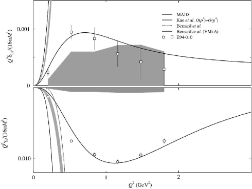
4 SUMMARY, OUTLOOK AND CONCLUSIONS

Recent advances in polarized electron sources, polarized nucleon targets and nucleon recoil polarimeters have enabled accurate measurements of the spin-dependent elastic electron-nucleon cross section. New data on nucleon electro-magnetic form factors with unprecedented precision have (and will continue to) become available in an ever increasing $Q^{2}{}$-domain. The two magnetic form factors $G_{M}^{p}$ and $G_{M}^{n}{}$ closely follow the simple dipole form factor $G_{D}$. $G_{E}^{p}/G_{M}^{p}$ drops linearly with $Q^{2}{}$  and $G_{E}^{n}$ appears to drop at the same rate as $G_{E}^{p}$ from $\sim 1$ GeV² onwards. The $Q^{2}{}$-behavior of $G_{E}^{p}$ has provided a signal of substantial non-zero orbital angular momentum in the proton. Only scant data are available in the time-like region. The full EMFF data set forms tight constraints on models of nucleon structure. So far, all available theories are at least to some extent effective (or parametrizations). Still, only few of these adequately describe all four EMFFs. Only lattice gauge theory can provide a truely ab initio calculation, but accurate lattice QCD results for the EMFFs are still several years away. A scaling prediction has been developed for the ratio of the Pauli and Dirac form factors, which the data appear to follow even at a $Q^{2}{}$-value as low as 1 GeV². Novel procedures allow a visualization of the nucleon structure as a function of the momentum of the struck quark. A fully three-dimensional picture of the nucleon will become available when future exclusive data have allowed the determination of the Generalized Parton Distributions.

Measurements of the nucleon polarizabilities have followed a 40-year odyssey that parallels the history of form-factor measurements. Powerful new theoretical and experimental techniques allow high precision measurements of the polarizablities and their $Q^{2}$-dependent generalizations. These results offer new evidence for the interplay of constituent quark and pion degrees of freedom at modest distance scales within the nucleon, and the dynamics of the elementary current quarks of QCD at large $Q^{2}$. This program will continue with both existing and future experimental facilities.

References

- [1] Frisch R, Stern O. Z. Phys. 85:4 (1933); Estermann I, Stern O. Z. Phys. 85:17 (1933)
- [2] Hofstadter R. Ann. Rev. Nucl. Science 7:231 (1957)
- [3] Wilson RR, Levinger JS. Ann. Rev. Nucl. Science 14:135 (1964)
- [4] Rosenbluth MN. Phys. Rev. 79:615 (1950)
- [5] Hofstadter R, Bumiller F, Croisseaux M. Phys. Rev. Lett. 5:263 (1960)
- [6] Hand LN, Miller DG, Wilson R. Rev. Mod. Phys. 35:335 (1960)
- [7] Ernst FJ, Sachs RG, Wali KC. Phys. Rev. 119:1105 (1960)
- [8] Bosted P, et al. Phys. Rev. C 51:409 (1995)
- [9] Janssens T, et al. Phys. Rev 142:922(1966)
- [10] Bartel W, et al. Phys. Rev. Lett. 17:608 (1966)
- [11] Litt J, et al. Phys. Lett. B 31:40 (1970) and references therein
- [12] Berger C, et al. Phys. Lett. B 35:87 (1971)
- [13] Walker RC, et al. Phys. Rev. D 49:5671 (1994)
- [14] Andivahis L, et al. Phys. Rev. D 50:5491 (1994)
- [15] Akhiezer AI, Rozentsweig LN, Shmushkevich IM. Sov. Phys. JETP 6:588 (1958)
- [16] Arnold R, Carlson C, Gross F. Phys. Rev. C 23:363 (1981)
- [17] Aulenbacher K. Proc. 9th Int. Workshop on Polarized Sources and Targets, p. 141. Singapore: World Scientific (2002)
- [18] Derbenev YaS, Kondratenko AM. Sov. Phys. JETP 37:968 (1973)
- [19] Steigerwald M. Proc. 14th Int. Workshop on Polarized Sources, AIP Conf. Proc. vol. 570, p. 935. New York: American Institute of Physics (2001)
- [20] Hauger M, et al. Nucl. Instrum. Methods A 462:382 (2001)
- [21] Baylac M, et al. Phys. Lett. B 459:412 (2001)
- [22] Chudakov E. Luppov V. Proc. 2003 IEEE Nuclear Science Symposium, IEEE Trans. on Nucl Science 51:1533 (2004)
- [23] Crabb D, et al. Nucl. Instrum. Methods A 356:9 (1995); Averett TD, et al. Nucl. Instrum. Methods A 427:440 (1999)
- [24] Steffens E, Haeberli W. Rep. Prog. Phys. 66:1887 (2003)
- [25] Clasie B, et al. Presented at X-th Workshop on Polarized Sources and Targets, Novosibirsk, 2003
- [26] Golak J, et al. Phys. Rev. C 63:034006 (2001)
- [27] Sargsian M. Int. J. Mod. Phys. E 10:405 (2001)
- [28] Alcorn J, et al. Nucl. Instrum. Methods A 522:294 (2004)
- [29] Surkau R, et al. Nucl. Instrum. Methods A 384:444 (1997)
- [30] Ostrick M, et al. Phys. Rev. Lett. 83:276 (1999)
- [31] Perdrisat C, Punjabi V, spokespersons. Jefferson Lab experiment E89-014 (1989)
- [32] Milbrath B, et al. Phys. Rev. Lett. 80:452 (1998); erratum, Phys. Rev. Lett. 82:2221 (1999)
- [33] Pospischil T, et al. Eur. Phys. Jour. A 12:125 (2001)
- [34] Punjabi V, et al. Phys. Rev. C 71:055202 (2005); Jones MK, et al. Phys. Rev. Lett. 84:1398 (2000)
- [35] Gayou O, et al. Phys. Rev. Lett. 88:092301 (2002)
- [36] Dieterich S, et al. Phys. Lett. B 500:47 (2001)
- [37] Christy ME, et al. Phys. Rev. C 70:015206 (2004)
- [38] Arrington J. Phys. Rev. C 68:034325 (2003)
- [39] Qattan IA, et al. Phys. Rev. Lett. 94:142301 (2005)
- [40] Offermann EAJM, et al. Phys. Rev. C 44:1096 (1991)
- [41] Mo LW, Tsai YS. Rev. Mod. Phys. 41:205 (1969); Maximon LC, Tjon JA. Phys. Rev. C 62:054320 (2000)
- [42] Guichon PAM, Vanderhaeghen M. Phys. Rev. Lett. 91:142303 (2003)
- [43] Arrington J. Phys. Rev. C 69:022201R (2004)
- [44] Arrington J. Phys. Rev. C 69:032201R (2004) and references therein
- [45] Blunden PG, Melnitchouk, Tjon JA. Phys. Rev. Lett. 91:142304 (2003)
- [46] Chen YC, et al. Phys. Rev. Lett. 93:122301 (2004)
- [47] Brooks, et al., spokespersons. Jefferson Lab experiment PR-04-116 (2004)
- [48] Borkowski F, et al. Nucl. Phys. B 93:461 (1975)
- [49] Bosted PE, et al. Phys. Rev. C 42:38 (1990)
- [50] Sill AF, et al. Phys. Rev. D 48:29 (1993)
- [51] Brash E, et al. Phys. Rev. C 65:051001 (2002)
- [52] Rock S, et al. Phys. Rev. D 46:24 (1992)
- [53] Anklin H, et al. Phys. Lett. B 336:313 (1994)
- [54] Anklin H, et al. Phys. Lett. B 428:248 (1998)
- [55] Kubon G, et al. Phys. Lett. B 524:26 (2002)
- [56] Bruins EEW, et al. Phys. Rev. Lett. 75:21 (1995)
- [57] Brooks M, Vineyard MF, spokespersons. Jefferson Lab experiment E94-017 (1994); private communication
- [58] Donnelly TW, Raskin AS. Ann. Phys. 169:247 (1986)
- [59] Gao H, et al. Phys. Rev. C 50:R546 (1994)
- [60] Xu W, et al. Phys. Rev. Lett. 85:2900 (2000)
- [61] Xu W, et al. Phys. Rev. C 67:012201R (2003)
- [62] Arnold R, et al. Phys. Rev. Lett. 61:806 (1988)
- [63] Lung AF, et al. Phys. Rev. Lett. 70:718 (1993)
- [64] Markowitz P, et al. Phys. Rev. C 48:R5 (1993)
- [65] Platchkov S, et al. Nucl. Phys. A 510:740 (1990)
- [66] Eden T, et al. Phys. Rev. C 50:R1749 (1994)
- [67] Passchier I, et al. Phys. Rev. Lett. 82:4988 (1999)
- [68] Herberg C, et al. Eur. Phys. Jour. A 5:131 (1999)
- [69] Madey R, et al. Phys. Rev. Lett. 91:122002 (2003)
- [70] Glazier DI, et al. Eur. Phys. Jour. A 24:101 (2005)
- [71] Warren G, et al. Phys. Rev. Lett. 92:042301 (2004); Zhu H, et al. Phys. Rev. Lett. 87:081801 (2001)
- [72] Jones-Woodward CE, et al. Phys. Rev. C 44:R571 (1991)
- [73] Becker J, et al. Eur. Phys. Jour. A 6:329 (1999)
- [74] Bermuth J, et al. Phys. Lett. B 564:199 (2003); Rohe D, et al. Phys. Rev. Lett. 83:4257 (1999)
- [75] Schiavilla R, Sick I. Phys. Rev. C 64:041002 (2001)
- [76] Galster S, et al. Nucl. Phys. B 32:221 (1971)
- [77] Iachello F, Wan Q. Phys. Rev. C 69:055204 (2004)
- [78] Hammer HW, Meissner UG, Drechsel D. Phys. Lett. B 385:343 (1996)
- [79] Dubnicka S, Dubnickova AZ, Weisenpacher P. J. Phys. G: Nucl. Part. Phys. 29:405 (2003)
- [80] Perdrisat CF, et al., spokespersons. Jefferson Lab experiment E01-109 (2001)
- [81] Wojtsekhowski B, et al., spokespersons, Jefferson Lab experiment E02-013 (2002)
- [82] Gao H, Calarco JR, Kolster H, spokespersons. MIT-Bates proposal 01-01 (2001)
-
[83]
Pre-Conceptual Design Report for the Science and Experimental Equipment for the 12 GeV Upgrade of CEBAF, 2003, Cardman LS, et al., editors,
http://www.jlab.org/div_dept/physics
_division/pCDR_public/pCDR_12-1 - [84] Sick I. Phys. Lett. B 576:62 (2003); private communication (2004)
- [85] Melnikov K, van Ritbergen T. Phys. Rev. Lett. 84:1673 (2000)
- [86] Kopecky S, et al. Phys. Rev. C 56:2229 (1997)
- [87] Isgur N. Phys. Rev. Lett. 83:272 (1999);
- [88] Kelly JJ. Phys. Rev. C 66:065203 (2002)
- [89] Friedrich J, Walcher Th. Eur. Phys. Jour. A 17:607 (2003)
- [90] Hammer HW, Drechsel D, Meissner UG. Phys. Lett. B 586:291 (2004)
- [91] Thomas AW and Weise W. The Structure of the Nucleon, Berlin: Wiley-VCH (2001)
- [92] Iachello F, Jackson A and Lande A, Phys. Lett. B 43:191 (1973)
- [93] Gari MF, Krümpelmann W. Z. Phys. A 322:689 (1985); Phys. Lett. B 274:159 (1992)
- [94] Lomon EL. Phys. Rev. C 64:035204 (2001); Phys. Rev. C 66:045501 (2002)
- [95] Höhler G, et al. Nucl. Phys. B 114:505 (1976)
- [96] Hammer HW, Meissner UG. Eur. Phys. Jour. A 20:469 (2004); Mergell P, Meissner UG, Drechsel D. Nucl. Phys. A 596:367 (1996)
- [97] Bijker R, Iachello F. Phys. Rev. C 69:068201 (2004)
- [98] Fuchs T, Gegelia J, Scherer S. Eur. Phys. Jour. A 19 (Suppl. 1):35 (2004) and references therein
- [99] Miller GA. Phys. Rev. C 66:032001R (2002)
- [100] Théberge S, Thomas AW, Miller GA. Phys. Rev. D 24:216 (1981)
- [101] Schlumpf F. J. Phys. G 20:237 (1994)
- [102] Cardarelli F, Simula S. Phys. Rev. C 62:065201 (2000)
- [103] Petronzio R, Simula S, Ricco G. Phys. Rev. D 67:094004 (2003)
- [104] Wagenbrunn RF, et al. Phys. Lett. B 511:33 (2001); Boffi S, et al. Eur. Phys. Jour. A 14:17 (2002)
- [105] Desplanques B, Theussl L. hep-ph/0307028
- [106] Coester F, Riska DO. Nucl. Phys. A 728:439 (2003)
- [107] Giannini M, Santopinto E, Vassallo A. Prog. Part. Nucl. Phys. 50:263 (2003); De Sanctis M, et al. Phys. Rev. C 62:025208 (2000); Ferraris M, et al. Phys. Lett. B 364:231 (1995)
- [108] Merten D, et al. Eur. Phys. Jour. A 14:477 (2002)
- [109] Van Cauteren T, et al. Eur. Phys. Jour. A 20:283 (2004)
- [110] Holzwarth G. Z. Phys. A 356:339 (1996); hep-ph/0201138
- [111] Kim HC, et al. Phys. Rev. D 53:4013 (1996); Christov CV, et al. Nucl. Phys. A 592:513 (1995)
- [112] Brodsky SJ, Farrar G. Phys. Rev. D 11:1309 (1975)
- [113] Brodsky SJ, Lepage GP. Phys. Rev. D 24:2848 (1981)
- [114] Miller GA. Phys. Rev. C 65:065205 (2002)
- [115] Ralston JP, Jain P. Phys. Rev. D 69:053008 (2004)
- [116] Brodsky SJ, et al. Phys. Rev. D 69:076001 (2004)
- [117] Belitsky AV, Ji X, Yuan F. Phys. Rev. Lett. 91:092003 (2003)
- [118] Miller GA, Phys. Rev. C 68:022201R (2003)
- [119] Ji X. Phys. Rev. Lett. 91:062001 (2003)
- [120] Göckeler M, et al. Phys. Rev. D 71:034508 (2005)
- [121] Ashley JD, et al. Eur. Phys. Jour. A 19 (Suppl. 1):9 (2004)
- [122] Holstein BR, Drechsel D, Pasquini B, Vanderhaeghen M. Phys. Rev. C 61:034316 (2000)
- [123] Bardeen WA, Tung WK. Phys. Rev. 173:1423 (1968)
- [124] Petrunkin VA. Sov. J. Part. Nucl. 12:278 (1981)
- [125] Babusci D, et al. Phys. Rev. C 58:1013 (1998)
- [126] Powell JL. Phys. Rev. 75:32 (1949)
- [127] Klein O, Nishina Y. Z. Physik 52:853 (1929)
- [128] Drell SD, Hearn AC. Phys. Rev. Lett. 16:908 (1966)
- [129] Gerasimov SB. Sov. J. Nucl. Phys. 2:430 (1966)
- [130] Baldin AM, Nucl. Phys. 18:310 (1960)
- [131] Damashek M, Gilman FJ. Phys. Rev. D 1:1319 (1970)
- [132] Babusci D, Giordano G, Matone G. Phys. Rev. C 57:291 (1998)
- [133] L’vov AI. Int. J. Mod. Phys. A 8:5267 (1993)
- [134] Gol’danski VI, et al. Sov. Phys. JETP 11:1123 (1960).
- [135] Baranov PS, et al. Sov. J. Nucl. Phys. 21:355 (1975)
- [136] MacGibbon BE, et al. Phys. Rev. C 52:2097 (1995)
- [137] Hallin EL, et al. Phys. Rev. C 48:1497 (1993)
- [138] Zieger A, et al. Phys. Lett. B 278:34 (1992)
- [139] Federspiel FJ, et al. Phys. Rev. Lett. 67:1511 (1991)
- [140] Nathan A. Radiation Physics and Chemistry 56:113 (1999)
- [141] Olmos de Leon V, et al. Eur. Phys. J. A 10:207 (2001)
- [142] L’vov AI. Sov. J. Nucl. Phys. 34:597 (1981)
- [143] L’vov AI, Petrun’kin VA, Schumacher M. Phys. Rev. C 55:359 (1997).
- [144] Drechsel D, Gorchtein M, Pasquini B, Vanderhaeghen M. Phys. Rev. C 61:015204 (2000)
- [145] Drechsel D, Pasquini B, Vanderhaeghen M. Phys. Rept. 378:99 (2003)
- [146] Gell-Mann M, Goldberger ML, Thirring WE. Phys. Rev. 95:1612 (1954)
- [147] Gell-Mann M, Goldberger ML. Phys. Rev. 96:1433 (1954)
- [148] Sandorfi AM, Khandaker M, Whisnant CS. Phys. Rev. D 50:6681 (1994)
- [149] Ahrens J, et al. Phys. Rev. Lett. 87:022003 (2001)
- [150] Dutz H, et al. Phys. Rev. Lett. 91:192001 (2003)
- [151] Tiator L. Proc. 2nd Int. Symp. Gerasimov-Drell-Hearn Sum Rule and the Spin Structure of the Nucleon (GDH 2002), Genoa, Italy, 3-6 Jul 2002, p. 27, River Edge, N.J., World Scientific, 2003.
- [152] Tonnison J, Sandorfi AM, Hoblit S, Nathan AM. Phys. Rev. Lett. 80:4382 (1998)
- [153] Blanpied G, et al. Phys. Rev. C 64:025203 (2001)
- [154] Galler G, et al. Phys. Lett. B 503:245 (2001)
- [155] Wolf S, et al. Eur. Phys. J. A. 12:231 (2001)
- [156] Camen M, et al. Phys. Rev. C 65:032202 (2002)
- [157] Drechsel D, Hanstein O, Kamalov SS, Tiator L. Nucl. Phys. A 645:145 (1999)
- [158] Tiator L, et al. Eur. Phys. Jour. A 19:55 (2004)
- [159] Arndt RA, et al. Phys. Rev. C 66:055213 (2002)
- [160] Drechsel D, Krein G, Hanstein O. PLB 420:248 (1998)
- [161] L’vov AI, Nathan AM. Phys. Rev. C 59:1064 (1999)
- [162] Bernard V, et al. Nucl. Phys. B 388:315 (1992)
- [163] Bernard V, Kaiser N, Schmidt A, Meissner UG. Phys. Lett. B 319:269 (1993)
- [164] Bernard V, Kaiser N, Meissner UG, Schmidt A.V. Z. Phys. A 348:317 (1994)
- [165] Hemmert TR, Holstein BR and Kambor J. Phys. Rev. D 55:5598 (1997)
- [166] Ji XD, Kao CW, Osborne J. Phys. Rev. D 61:074003 (2000)
- [167] Kumar KBV, McGovern JA, Birse MC. Phys. Lett. B 479:167 (2000)
- [168] Gellas GC, Hemmert TR, Meissner UG. Phys. Rev. Lett. 85:14 (2000)
- [169] Birse MC, Ji XD, McGovern JA. Phys. Rev. Lett. 86:3204 (2001)
- [170] Gellas GC, Hemmert TR, Meissner UG. Phys. Rev. Lett. 86:3205 (2001)
- [171] Beane SR, et al. Phys. Lett. B 567:200 (2003)
- [172] McGovern JA. AIP Conf. Proc. 603:249 (2001)
- [173] Zhou L, et al. Nucl. Phys. Proc. Suppl. 119:272 (2003)
- [174] Christensen J, et al. Nucl. Phys. Proc. Suppl. 119:269 (2003)
- [175] Wissmann F, Schumacher M, Levchuk MI. Eur. Phys. J. A 1:193 (1998)
- [176] Schmiedmayer J, Rauch H, Riehs P. Phys. Rev. Lett. 66:1051 (1991)
- [177] Koester L, et al. Phys. Rev. C 51:3363 (1995)
- [178] Enik TL, et al. Phys. Atom. Nucl. 60:567 (1997), Yad. Fiz. 60:648 (1997)
- [179] Rose KW, et al. Phys. Lett. B 234:460 (1990)
- [180] Rose KW, et al. Nucl. Phys. A 514:621 (1990)
- [181] Hornidge DL, et al. Phys. Rev. Lett. 84:2334 (2000)
- [182] Kolb NR, et al. Phys. Rev. Lett. 85:1388 (2000)
- [183] Lundin M, et al. Phys. Rev. Lett. 90:192501 (2003)
- [184] Kossert K, et al. Phys. Rev. Lett. 88:162301 (2002)
- [185] Kossert K, et al. Eur. Phys. J. A 16:259 (2003)
- [186] Wissmann F, et al. Nucl. Phys. A 660:232 (1999)
- [187] Levchuk MI, L’vov AI, Petrunkin VA. Few-Body Syst. 16:101 (1994)
- [188] Levchuk MI, L’vov AI. Nucl. Phys. A 674:449 (2000)
- [189] Karakowski JJ, Miller GA. Phys. Rev. C 60:014001 (1999)
- [190] Guichon PA, Liu GQ, Thomas AW. Nucl. Phys. A 591:606 (1995)
- [191] L’vov AI, et al. Phys. Rev. C 64:015203 (2001)
- [192] Metz A, Drechsel D. Z. Phys. A 356:351 (1996)
- [193] Metz A, Drechsel D. Z. Phys. A 359:165 (1997)
- [194] Drechsel D, et al. Phys. Rev. C 55:424 (1997)
- [195] Drechsel D, et al. Phys. Rev. C 57:941 (1998)
- [196] Guichon PAM, Vanderhaeghen M. Prog. Part. Nucl. Phys. 41:125 (1998)
- [197] Roche J, et al. Phys. Rev. Lett. 85:708 (2000)
- [198] Vanderhaeghen M, et al. Phys. Rev. C 62:025501 (2000)
- [199] Liu GQ, Thomas AW, Guichon PAM. Austral. J. Phys. 49:905 (1996)
- [200] Pasquini B, Scherer S, Drechsel D. Phys. Rev. C 63:025205 (2001)
- [201] Vanderhaeghen M. Phys. Lett. B 368:13 (1996)
- [202] Vanderhaeghen M. Phys. Lett. B 402:243 (1997)
- [203] Kim M, Min DP. hep-ph/9704381
- [204] Hemmert TR, et al. Phys. Rev. Lett. 79:22 (1997)
- [205] Hemmert TR, et al. Phys. Rev. D 55:2630 (1997)
- [206] Hemmert TR, et al. Phys. Rev. D 62:014013 (2000)
- [207] Kao CW, Vanderhaeghen M. Phys. Rev. Lett. 89:272002 (2002)
- [208] Laveissière G, et al. Phys. Rev. Lett. 93:122001 (2004)
- [209] Pasquini B, et al. Eur. Phys. Jour. A 11:185 (2001)
- [210] Brasse FW, et al. Z. Phys. C 22:33 (1984)
- [211] Thompson R, et al. Phys. Rev. Lett. 86:1702 (2001)
- [212] Shaw J, Miskimen R, spokespersons. M.I.T.-Bates Experiment 97-03 (1997).
[213]
Bertin PY, et al.,
spokesperons. Jefferson Lab Experiment E93-050,
http://www.jlab.org/exp_prog/
generated/halla.html -
[214]
Laveissière G, et al., spokespersons.
Jefferson Lab Proposal P03-010,
generated/halla.html - [215] Hand LN. Phys Rev 129:1834 (1963).
- [216] Bjorken JD, Paschos EA. Phys Rev 185:1975 (1969)
- [217] Wandzura W, Wilczek F. Phys. Lett. B 72:195 (1977)
- [218] Osipenko M, et al. Phys. Rev. D 67:092001 (2003)
- [219] Armstrong CS, et al. Phys. Rev. D 63:094008 (2001)
- [220] Martin AD, et al. Phys. Lett. B 531:216 (2002)
- [221] Amarian M, et al. Phys. Rev. Lett. 92:022301 (2004)
- [222] Kao CW, Spitzenberg T, Vanderhaeghen M. Phys. Rev. D 67:016001 (2003)
- [223] Bernard V, Hemmert TR, Meissner UG. Phys. Rev. D 67:076008 (2003)
- [224] Liang Y, et al.. Proc. 3rd Int. Symposium on the GDH Sum Rule and its Extensions. Singapore: World Scientific (2005)
- [225] Amarian M, et al. Phys. Rev. Lett. 93:152301 (2004)