Quantifying Self-Organization in Cyclic Cellular Automata

Abstract

Cyclic cellular automata (CCA) are models of excitable media. Started from random initial conditions, they produce several different kinds of spatial structure, depending on their control parameters. We introduce new tools from information theory that let us calculate the dynamical information content of spatial random processes. This complexity measure allows us to quantitatively determine the rate of self-organization of these cellular automata, and establish the relationship between parameter values and self-organization in CCA. The method is very general and can easily be applied to other cellular automata or even digitized experimental data.

1 Introduction

The term “self-organization” was introduced in the 1940s [(1)], and become one of the leading concepts of nonlinear science, without, however, ever having received a proper characterization. The prevailing “I know it when I see it” standard actually impedes scientific progress, since it prevents our developing even the rudiments of a theory of self-organization. Thus some researchers state that “self-organizing” implies “dissipative” [(2)], and others claim to exhibit reversible systems that self-organize [(3)], and no one can even say if they are both talking about the same idea. It would be useful, therefore, to have a definition of self-organization which was mathematically precise, so we could build formal theories around it, and experimentally applicable, so that one could say whether or not something self-organizes on the basis of empirical data. Any such definition must be tested against cases where intuition is clear, preferably cases where we know exactly what is going on.

We believe we have such a definition of self-organization, and test it here against cellular automata, specifically the so-called cyclic cellular automata. We selected these systems for a number of reasons: their dynamics are completely known and can easily be simulated exactly, they are decent qualitative models of chemical waves, and there is already an analytical theory of the patterns they form, against which we can check our results.

2 Spiral Wave Formation in Cyclic Cellular Automata

Cyclic cellular automata [(4), (5)] (CCA) are caricatures of pattern formation in chemical oscillators and other excitable media [(6)]. Each site in a square two-dimensional lattice is in one of $\kappa$ colors. A cell of color $k$ will change its color to $k+1\bmod\kappa$ if there are already at least $T$ cells of that color in its neighborhood, i.e., within a distance $r$ of that cell. Otherwise, the cell retains its current color. (All cells update their color in parallel.)

The CCA has three generic forms of long-term behavior, depending on the size of the threshold relative to the range. At high thresholds, the CCA forms homogeneous blocks of solid colors, which are completely static — so-called fixation behavior. At very low thresholds, the entire lattice eventually oscillates periodically; sometimes the oscillation takes the form of large spiral waves which grow to engulf the entire lattice. There is an intermediate range of thresholds where incoherent traveling waves form, propagate for a while, and then disperse; this is called “turbulence”, but whether it has any connection to actual fluid turbulence is unknown. With a range one “Moore” (box) neighborhood, the phenomenology is as follows [(5)]. $T=1$ and $T=2$ are both locally periodic, but $T=2$ produces spiral waves, while $T=1$ “quenches” incoherent local oscillations. At $T=3$, one encounters “turbulence,” which is actually meta-stable — spiral waves can form and entrain the entire CA, but this does not always happen on finite lattices, and in any case the turbulent phase can persist for very long times. Fixation occurs with $T\geq 4$. Intuitively, all three phases of the CCA can be said to self-organize when started from uniform noise. Also intuitively, that is, by the “I know it when I see it” standard, the fixation phase is less organized than turbulence, which is less organized than spiral waves. It is hard to say, by eye, whether incoherent local oscillations are more or less organized than simple fixation.

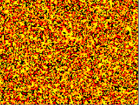
Figure 1: Local oscillations in the CCA $(T=1)$. In this and the subsequent figures, the number of colors is fixed to 4, the rule uses a range-one box-shaped neighborhood, and the initial conditions are a uniform random mixture of colors. These figures, but not our numerical results, were prepared using the MJCell program by Mirek Wójtowicz, http://psoup.math.wisc.edu/mcell/. Observe the slight departure from uniform randomness, in the shape of connected twisting single-color bands. The CA as a whole oscillates with period 4, each cell cycling through the colors.

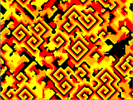
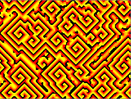
Figure 2: Spiral waves $(T=2)$ in the cyclic CA. Left: formation of spirals out of background regions, $t=45$. Right: the same system later ($t=200$), when the spirals have entrained the entire lattice.

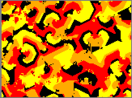
Figure 3: Typical view of the CCA “turbulent” phase $(T=3)$.

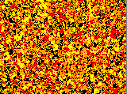
Figure 4: Fixation in the CCA $(T=4)$. Note that the configuration departs slightly from the random initial condition, owing to the growth of rectangular blocks of solid color.

3 A Measure of Organization

Few attempts have been made to measure self-organization quantitatively in either model or real systems. (See Refs. 7; 8 for reviews.) There is a widespread sense, perhaps first articulated by Bennett Bennett-dissipation ; Bennett-1986 ; Bennett-how-and-why , that self-organization is the same as a spontaneous increase in complexity, leaving us with the problem of measuring complexity. The obvious candidate, from a physical point of view, is thermodynamic entropy, and at least two studies have claimed to measure self-organization by measuring spontaneous declines over time in entropy Wolfram-stat-mech-CA ; Klimontovich . Unfortunately configurational or thermodynamic entropy is a most unsatisfying measure of organization in complex systems Medawar-general-evolution ; Fox-energy-evolution ; Badii-Politi ; DPF-JPC-why ; Sewell-emergent-macrophysics .

We shall expand on that last point, because it is not as well-appreciated as it should be. Thermodynamic entropy measures the degree of a system’s “mixedupedness” (to use Gibbs’s word), or how far it departs from being in a pure stateSewell-emergent-macrophysics . For many of the systems treated by statistical mechanics, pure states are more organized than impure ones, but there is no logical connection. Low-temperature spin systems may be in very pure states which have no significant organization. Organisms are essentially never in pure states, and are highly mixed up at the molecular level, but are the paradigmatic examples of organization. In fact, there are many instances of biological self-organization which are thermodynamically favored because they increase entropyMedawar-general-evolution ; Fox-energy-evolution . Furthermore, there are many different kinds of organization, and entropy ignores all the distinctions and gradations between themDPF-JPC-why .

So much for the idea that organization is simply “unmixedupedness”. Another school of thought, going back to KolmogorovKolmogorov-three-approaches and Solomonoff Solomonoff holds that complex phenomena are ones which do not admit of descriptions which are both short and accurate. The idea that complexity should be identified with long minimal descriptions has been implemented in many different ways Badii-Politi ; Li-and-Vitanyi-1993 . Many of these implementations remain in Kolmogorov’s original framework of exactly describing a particular configuration, and so inherit the feature that independent random configurations are hard to describe. (For the record of heads and tails from tossing a fair coin, the shortest algorithmic description is usually the sequence itself.) This is paradoxical from a stochastic point of view, where independent variables are the most basic kind available. The paradox may be resolved by changing our goal, to statistically describing ensembles of configurations.Rissanen-SCiSI (The heads-and-tails sequence is described as “independent Bernoulli trials with parameter $p=0.5$”, or, colloquially, “something you’d get by tossing a lot of coins”.) Within this general framework, the most satisfying version of the description-length idea defines the complexity of a process as the minimal amount of information about its state needed for maximally accurate prediction. Grassberger Grassberger-1986 first proposed this idea, and Crutchfield and Young Inferring-stat-compl gave operational definitions of “maximally accurate prediction” and “state”. For a full exposition of the resulting theory, as it applies to classical stochastic processes, see Ref. 25.

The Crutchfield-Young “statistical complexity”, $C_{\mu}$, of a dynamical process is the Shannon entropy (information content) of the minimal sufficient statistic for predicting the process’s future CMPPSS . In thermodynamic settings, this is just equal to the amount of information a full set of macrovariables contains about the microscopic state of the system CRS-thesis ; What-is-a-macrostate . For spatially extended systems, which are of interest here, it is more appropriate to look at the density of statistical complexity, using a refinement of the theory that handles local quantities, which we briefly sketch here, following Ref. 8.

3.1 Minimal Local Sufficient Statistics

Take a random field varying over space and time $X(\vec{r},t)$, where there is some maximum speed $c$ at which information can propagate. The past light cone of the space-time point $(\vec{r},t)$ consists of all points which could influence $X(\vec{r},t)$, i.e., all points $(\vec{s},u)$ such that $u<t$ and $|\vec{s}-\vec{r}|\leq c(t-u)$. Similarly, the future light cone of $(\vec{r},t)$ is the set of all points which could be influenced by what happens there. Write $L^{-}(\vec{r},t)$ for the configuration of the random field in the past light cone, and ${L}^{+}(\vec{r},t)$ for the configuration in the future light cone. (We will suppress the arguments except when comparing cones at different locations.) There is a certain distribution over future light-cone configurations conditional on the configuration in the past. The full notation for this would be ${\rm P}({L}^{+}|L^{-}=l^{-})$, but we shall abbreviate it as ${\rm P}({L}^{+}|l^{-})$.

Any function $\eta$ of $L^{-}$ defines a local statistic or local effective state. It can be thought of as summarizing the influence of all the space-time points which could affect what happens at $(\vec{r},t)$. Such local statistics should tell us something about “what comes next,” which is ${L}^{+}$. In fact, we can use information theory to quantify how informative different statistics are.

The Shannon entropy or information content of a random variable $Z$ is

$$H[Z] \equiv -\sum_{z}{{\rm P}(Z=z)\log_{2}{{\rm P}(Z=z)}}$$ (1)

$$= -\left<\log_{2}{{\rm P}(Z)}\right>~{},$$ (2)

which is the average number of bits needed to encode the value of $Z$. Equivalently, $H[Z]$ indicates how much uncertainty an ideal statistician would have about $Z$. The conditional entropy of $Z$ given $Y$,

$$H[Z|Y] \equiv -\sum_{y}{{\rm P}(Y=y)\sum_{z}{{\rm P}(Z=z|Y=y)\log_{2}{{\rm P}(Z=z|Y=y)}}}$$ (3)

$$= -\left<\log_{2}{{\rm P}(Z|Y)}\right>~{},$$ (4)

is the average number of bits needed to encode $Z$ if one knows $Y$. Hence the reduction in uncertainty, or description length, due to a knowledge of $Y$ is

$$I[Z;Y] \equiv H[Z]-H[Z|Y]$$ (5)

$$= \left<\log_{2}{\frac{{\rm P}(Z,Y)}{{\rm P}(Z){\rm P}(Y)}}\right>~{},$$ (6)

called the mutual information shared by $Z$ and $Y$.

For our case, we want to consider the information a local statistic $\eta$ conveys about the future, which is $I[{L}^{+};\eta(L^{-})]$. A statistic is sufficient if it is as informative as possibleKullback-info-theory-and-stats . In this case, a statistic $\eta$ is sufficient if and only if $I[{L}^{+};\eta(L^{-})]=I[{L}^{+};L^{-}]$, i.e., if it retains all the predictive information in the complete past. This in turn is equivalent to requiring that ${\rm P}({L}^{+}|\eta(l^{-}))={\rm P}({L}^{+}|l^{-})$, for all past configurations. Put slightly differently, given a sufficient statistic, one does not need to remember the data from which one computed it.

All sufficient statistics have the same predictive ability, but they are not equal in the resources they need to make that prediction. In particular, if one is using the local statistic $\eta$ to make predictions, one must describe or encode $\eta$, which takes $H[\eta(L^{-})]$ bits. If knowing the value of one statistic, say $\eta_{1}$, lets us determine the value of another, $\eta_{2}$, then intuitively $\eta_{2}$ is a more concise summary, and in fact $H[\eta_{1}(L^{-})]\geq H[\eta_{2}(L^{-})]$. A minimal local sufficient statisticKullback-info-theory-and-stats is one whose value can be determined from any other sufficient statistic. Unsurprisingly, minimal local sufficient statistics minimize the entropy $H[\eta(L^{-})]$. How can we construct a minimal statistic?

Take any two past light-cone configurations, $l^{-}_{1}$ and $l^{-}_{2}$. Each has some conditional distribution over future light-cone configurations, ${\rm P}({L}^{+}|l^{-}_{1})$ and ${\rm P}({L}^{+}|l^{-}_{2})$ respectively. Say that the two past configurations are equivalent, $l^{-}_{1}\sim l^{-}_{2}$ if those conditional distributions are equal. Then for each past configuration $l^{-}$, there is a set of configurations which are equivalent to it, which we may write $[l^{-}]$. Finally, consider the function which maps past configurations to their equivalence classes under the relation $\sim$:

$$\epsilon(l^{-}) \equiv [l^{-}]$$ (7)

$$= \left\{\lambda\left|{\rm P}({L}^{+}|\lambda)={\rm P}({L}^{+}|l^{-})\right.\right\}$$ (8)

Clearly, ${\rm P}({L}^{+}|\epsilon(l^{-}))={\rm P}({L}^{+}|l^{-})$, and so $I[{L}^{+};\epsilon(L^{-})]=I[{L}^{+};L^{-}]$, making $\epsilon$ a sufficient statistic. The equivalence classes, the values $\epsilon$ can take, are called the (local) causal statesInferring-stat-compl ; CMPPSS . Each causal state corresponds to a distinct conditional distribution for the contents of the future light-cone. We write the causal state at $(\vec{r},t)$ as $S(\vec{r},t)$.

We saw already that ${\rm P}({L}^{+}|l^{-})={\rm P}({L}^{+}|\eta(l^{-}))$, for any sufficient statistic $\eta$. So if $\eta(l^{-}_{1})=\eta(l^{-}_{2})$, then ${\rm P}({L}^{+}|l^{-}_{1})={\rm P}({L}^{+}|l^{-}_{2})$, and the two pasts belong to the same causal state. Hence, if we know the value of $\eta(l^{-})$, we can determine the value of $\epsilon(l^{-})$. But this means that $\epsilon$ is a minimal sufficient statistic. Moreover, one can showCRS-thesis that $\epsilon$ is the unique minimal sufficient statistic, in the sense that any other minimal statistic is just a relabeling of the same set of states.

Because $\epsilon$ is a minimal sufficient statistic, $H[\epsilon(L^{-})]\leq H[\eta(L^{-})]$, for any other sufficient statistic $\eta$. This being the case, we are entitled to speak, in an objective manner, about the minimal amount of information needed to predict the system, or, as we may also think of it, how much information the system retains from its past. This quantity, $H[S]$ is a characteristic of the system, and not (just) of a particular class of model. We therefore write $C_{\mu}\equiv H[S]$, and call this the statistical complexity density; we will frequently drop the “density”. $C_{\mu}$ is the amount of information about the past light-cone which the system’s dynamics make relevant to the future.

We now propose to define self-organization thus: a system has self-organized between time $t_{1}$ and time $t_{2}$ if (1) $C_{\mu}(t_{1})<C_{\mu}(t_{2})$, and (2) not all of the increase in complexity is due to outside intervention. Clearly, if the system is not being manipulated from the outside at all, (2) doesn’t matter, and this is true of many systems which either have no interaction with the outside world (e.g., deterministic CAs), or whose only inputs are zero-memory noise (e.g., stochastic CAs, or laboratory chemical pattern formers subject to thermal noise). In the case of systems subject to structured input, clearly one would like to divide increases in complexity into a portion due to the input and a portion due to the self-organizing dynamics of the system. There is not yet any obvious way to do this, though the “potential response” methods of statistical inferenceHolland-on-Rubin may help.

It is appropriate, at this point, to take a step back and consider what we are doing. Why should we use the light-cone construction, as opposed to any other kind of localized predictor? Indeed, why use localized statistics at all? Let us answer these in reverse order. The use of local predictors is partly a matter of interest — in studying self-organization, we care deeply about spatial structure, and so global approaches, which would treat the system’s sequence of configurations as one giant time series, simply don’t tell us what we want to know. In part, too, the local approach makes a virtue of necessity, because global prediction quickly becomes impractical for systems of any real size. The number of modes required by methods attempting global prediction, like Karhunen-Loeve decomposition, grows extensively with system volumeZoldi-Greenside-extensive-chaos ; Zoldi-et-al-extensive-scaling . There is thus no advantage in terms of compression or accuracy to global methods.

The use of light-cones for the local predictors, rather than some other shape, is motivated partly by physical considerations, and partly the nice formal features which follow from the shape, of which we will mention threeCRS-thesis .

1. The light-cone causal states, while local statistics, do not lose any global predictive power. To be precise, if we specify the causal state at each point in a spatial region, that array of states is itself a sufficient statistic for the future configuration of the region, even if the region is the entire lattice.

2. The light-cone states can be found by a recursive filter. To illustrate what this means, consider two space-time points, $(\vec{r},t)$ and $(\vec{q},u)$, $u\geq t$. The state at each point is determined by the configuration in its past light-cone: $s(\vec{r},t)=\epsilon(l^{-}(\vec{r},t))$, $s(\vec{q},u)=\epsilon(l^{-}(\vec{q},u))$. The recursive-filtration property means that we can construct a function which will give us $s(\vec{q},u)$ as a function of $s(\vec{r},t)$, plus the part of the past light-cone of $(\vec{q},u)$ that is not visible from $(\vec{r},t)$. Not only does this greatly simplify state estimation, it opens up powerful connections to the theory of two-dimensional automataTwo-D-Patterns .

3. The local causal states form a Markov random field, once again allowing very powerful analytical techniques to be employed which would not otherwise be available.

In general, if we used some other shape than the light-cones, we would not retain any of these properties.

4 Methods and Results

We ran the four-color, range-one CCA on a $100\times 100$ lattice with wrap-around boundary conditions at four different values of the $T$ parameter. Recall that at $T=2$, the system strongly self-organizes into spiral waves, that $T=3$ is also felt to be self-organizing but not as much, and that $T=1$ and $T=4$ show significantly less self-organization. All four regimes lead to stable stationary distributions. We therefore expect $C_{\mu}$ to start at zero (reflecting the uniform random initial conditions), and then rise to a steady value which it maintains forever. The long-run complexity should be highest for $T=2$, lower for $T=3$, and much smaller for $T=1$ or $T=4$.

For our present purposes, where we are just interested in $C_{\mu}(t)$, it is fairly straightforward to devise an algorithm to reconstruct the local causal states from data. At each time $t$, we determine which past and future light-cone configurations are actually observed in the data. Then, for each past configuration $l^{-}$, we estimate ${\rm P}_{t}({L}^{+}|l^{-})$, treated simply as a multinomial distribution. We then cluster past configurations based on the similarity of their conditional distributions. We cannot expect that the estimated distributions will match exactly, so we employ a simple $\chi^{2}$ test (with $\alpha=0.05$) to determine whether the discrepancy between estimated distributions is significant. These clusters are then the estimated local causal states. We consider each cluster to have a conditional distribution of its own, equal to the weighted mean of the distributions of the pasts it contains. Finally, we obtain the probabilities of the different states $s_{i}$ from those of their constituent past configurations, and so calculate $-\sum_{i}{{\rm P}(s_{i})\log_{2}{{\rm P}(s_{i})}}$ = $C_{\mu}(t)$.

As a practical matter, we need to impose a limit on how far back into the past, or forward into the future, the light-cones are allowed to extend — their depth. Also, clustering cannot be done on the basis of a true equivalence relation. Instead, we list the past configurations $\left\{l^{-}_{i}\right\}$ in some arbitrary order. We then create a cluster which contains the first past, $l^{-}_{1}$. For each later past, say $l^{-}_{i}$, we go down the list of existing clusters and check whether ${\rm P}_{t}({L}^{+}|l^{-}_{i})$ differs significantly from each cluster’s distribution. If there is no difference, we add $l^{-}_{i}$ to the first matching cluster and update the latter’s distribution. If $l^{-}_{i}$ does not match any existing cluster, we make a new cluster for $l^{-}_{i}$. (See Figure 5 for pseudo-code.) As we give this procedure more and more data, it converges in probability on the correct set of causal states, independent of the order in which we list past light-conesCRS-thesis . For finite data, the order of presentation matters, but we finesse this by randomizing the order.

U $\leftarrow$ list of all pasts in random order
Move the first past in U to a new state
for	each past in U
	noMatch $\leftarrow$ TRUE
	state $\leftarrow$ first state on the list of states
	while	(noMatch and more states to check)
		noMatch $\leftarrow$ (Significant difference between past and state?)
		if	(noMatch)
			state $\leftarrow$ next state on the list
		else
			Move past from U to state
			noMatch $\leftarrow$ FALSE
	if	(noMatch)
		make a new state and move past into it from U

Figure 5: Algorithm for grouping past light-cones into estimated states

Our actual numerical results, averaged over 10 independent simulations at each value of $T$, are shown in Figure 6. They are clearly in agreement with what we would expect if $C_{\mu}$ actually does measure self-organization. All four curves climb monotonically to steady plateaus, leveling off when the CA configurations become stationary. The small fluctuations in the complexity in the stationary regimes are due to sampling effects — the lack of exact transitivity due to finite data inaccuracies in the estimated conditional distributions.

Figure 6: Complexity over time for CCA with different thresholds $T$. Error bars represent one standard deviation in the complexity; fluctuations are due to sampling effects, as described in the text.

5 Conclusions

5.1 Directions for Future Work

Clearly, this is just a first step towards establishing an acceptable criterion for self-organization. At the very least these results should be replicated for other cellular automata, such as pattern-forming lattice gasesRothman-Zaleski-text and voter modelsLiggett-particle-systems . Beyond cellular automata, our methods are applicable, with minor modifications, to all kinds of discrete random fields, including fields on arbitrary graphs, such as the recently-popular “complex networks” MEJN-on-network-structure-and-function . On an irregular graph, the shape of the light-cones will generally vary from node to node, so each node will have its own set of causal states, but it will still be possible to calculate $C_{\mu}$ over the graph, and so apply the basic ideas set out here.

Another obvious extension is to work with experimental data. Digital video provides discrete-valued data on regular, discrete lattices, and as such is eminently suited to our approach. Ultimately, one would like to be able to predict when, and how much, different physical systems will self-organize and actually validate those predictions with experimental data. While there are important issues in choosing appropriate discretizations Badii-Politi , there does not seem to be any obstacle, in principle, to doing so.

5.2 Summary

It would be nice to have a general theory of self-organization. Before work on that theory can begin, we need a mathematical characterization of self-organization, preferably one which can be applied to data directly. “Decline in thermodynamic entropy” is not really suited for this role, but “increase in complexity” is. We have shown how to define a sensible complexity measure for spatio-temporal systems, based on the amount of information actually required for optimal statistical prediction. This statistical complexity, $C_{\mu}$, can be reliably and straight-forwardly estimated from data. In the particular case of cyclic cellular automata, where the qualitative behavior changes drastically with the threshold parameter $T$, we find that whether or not $C_{\mu}$ increases over time agrees completely with intuitive judgments about self-organization.

- (1) W. R. Ashby, “Principles of the self-organizing dynamic system,” Journal of General Psychology 37, pp. 125–128, 1947.
- (2) G. Nicolis and I. Prigogine, Self-Organization in Nonequilibrium Systems: From Dissipative Structures to Order through Fluctuations, John Wiley, New York, 1977.
- (3) R. M. D’Souza and N. H. Margolus, “Thermodynamically reversible generalization of diffusion limited aggregation,” Physical Review E 60, pp. 264–274, 1999. URL http://arxiv.org/abs/cond-mat/9810258.
- (4) R. Fisch, J. Gravner, and D. Griffeath, “Cyclic cellular automata in two dimensions,” in Spatial Stochastic Processes: A Festschrift in Honor of Ted Harris on His Seventieth Birthday, K. Alexander and J. Watkins, eds., pp. 171–188, Birkhäuser, Boston, 1991. URL http://psoup.math.wisc.edu/papers/cca.zip.
- (5) R. Fisch, J. Gravner, and D. Griffeath, “Threshold-range scaling of excitable cellular automata,” Statistics and Computing 1, pp. 23–39, 1991. URL http://psoup.math.wisc.edu/papers/tr.zip.
- (6) A. T. Winfree, When Time Breaks Down: The Three-Dimensional Dynamics of Electrochemical Waves and Cardiac Arrhythmias, Princeton University Press, Princeton, 1987.
- (7) C. Gershenson and F. Heylighen, “When can we call a system self-organizing?” E-print, 2003. URL http://arxiv.org/abs/nlin.AO/0303020.
- (8) C. R. Shalizi, Causal Architecture, Complexity and Self-Organization in Time Series and Cellular Automata. PhD thesis, University of Wisconsin-Madison, 2001. URL http://bactra.org/thesis/.
- (9) C. H. Bennett, “Dissipation, information, computational complexity and the definition of organization,” in Emerging Syntheses in Science, D. Pines, ed., pp. 215–234, Santa Fe Institute, Santa Fe, New Mexico, 1985.
- (10) C. H. Bennett, “On the nature and origin of complexity in discrete, homogeneous locally-interacting systems,” Foundations of Physics 16, pp. 585–592, 1986.
- (11) C. H. Bennett, “How to define complexity in physics, and why,” in Complexity, Entropy, and the Physics of Information, W. H. Zurek, ed., pp. 137–148, Addison-Wesley, Reading, Massachusetts, 1990.
- (12) S. Wolfram, “Statistical mechanics of cellular automata,” Reviews of Modern Physics 55, pp. 601–644, 1983. Reprinted in [35].
- (13) Y. L. Klimontovich, Turbulent Motion and the Structure of Chaos: A New Approach to the Statistical Theory of Open Systems, Kluwer Academic, Dordrecht, 1990/1991. Translated by Alexander Dobroslavsky from Turbulentnoe dvizhenie i struktura khaosa: Novyi podkhod k statisticheskoi teorii otkrytykh sistem (Moscow: Nauka).
- (14) P. B. Medawar, Pluto’s Republic, pp. 209–227, Oxford University Press, Oxford, 1982.
- (15) R. F. Fox, Energy and the Evolution of Life, W. H. Freeman, New York, 1988.
- (16) R. Badii and A. Politi, Complexity: Hierarchical Structures and Scaling in Physics, Cambridge University Press, Cambridge, 1997.
- (17) D. P. Feldman and J. P. Crutchfield, “Measures of statistical complexity: Why?,” Physics Letters A 238, pp. 244–252, 1998.
- (18) G. L. Sewell, Quantum Mechanics and Its Emergent Macrophysics, Princeton University Press, Princeton, New Jersey, 2002.
- (19) A. N. Kolmogorov, “Three approaches to the quantitative definition of information,” Problems of Information Transmission 1, pp. 1–7, 1965.
- (20) R. J. Solomonoff, “A formal theory of inductive inference,” Information and Control 7, pp. 1–22 and 224–254, 1964. URL http://world.std.com/rjs/pubs.html.
- (21) M. Li and P. M. B. Vitanyi, An Introduction to Kolmogorov Complexity and Its Applications, Springer-Verlag, New York, 1993.
- (22) J. Rissanen, Stochastic Complexity in Statistical Inquiry, World Scientific, Singapore, 1989.
- (23) P. Grassberger, “Toward a quantitative theory of self-generated complexity,” International Journal of Theoretical Physics 25, pp. 907–938, 1986.
- (24) J. P. Crutchfield and K. Young, “Inferring statistical complexity,” Physical Review Letters 63, pp. 105–108, 1989.
- (25) C. R. Shalizi and J. P. Crutchfield, “Computational mechanics: Pattern and prediction, structure and simplicity,” Journal of Statistical Physics 104, pp. 817–879, 2001. URL http://arxiv.org/abs/cond-mat/9907176.
- (26) C. R. Shalizi and C. Moore, “What is a macrostate? from subjective measurements to objective dynamics.” E-print, 2003. URL http://arxiv.org/abs/cond-mat/0303625.
- (27) S. Kullback, Information Theory and Statistics, Dover Books, New York, 2nd ed., 1968. First edition New York: Wiley, 1959.
- (28) P. W. Holland, “Statistics and causal inference,” Journal of the American Statistical Association 81, pp. 945–970, 1986.
- (29) S. M. Zoldi and H. S. Greenside, “Karhunen-Loeve decomposition of extensive chaos,” Physical Review Letters 78, pp. 1687–1690, 1997. URL http://arxiv.org/abs/chao-dyn/961007.
- (30) S. M. Zoldi, J. Liu, K. M. S. Bajaj, H. S. Greenside, and G. Ahlers, “Extensive scaling and nonuniformity of the Karhunen-Loeve decomposition for the spiral-defect chaos state,” Physical Review E 58, pp. 6903–6906, 1998. URL http://arxiv.org/abs/chao-dyn/9808006.
- (31) K. Lindgren, C. Moore, and M. Nordahl, “Complexity of two-dimensional patterns,” Journal of Statistical Physics 91, pp. 909–951, 1998. URL http://arxiv.org/abs/cond-mat/9804071.
- (32) D. H. Rothman and S. Zaleski, Lattice-Gas Cellular Automata: Simple Models of Complex Hydrodynamics, Cambridge University Press, Cambridge, England, 1997.
- (33) T. M. Liggett, Interacting Particle Systems, Springer-Verlag, Berlin, 1985.
- (34) M. E. J. Newman, “The structure and function of complex networks,” SIAM Review 45, pp. 167–256, 2003. URL http://arxiv.org/abs/cond-mat/0303516.
- (35) S. Wolfram, Cellular Automata and Complexity: Collected Papers, Addison-Wesley, Reading, Massachusetts, 1994. URL http://www.stephenwolfram.com/publications/books/ca-reprint/.