Proton elastic form factor ratios to $Q^{2}$ = 3.5 GeV² by polarization transfer

Abstract

The ratio of the proton elastic electromagnetic form factors, $G_{Ep}/G_{Mp}$, was obtained by measuring $P_{t}$ and $P_{\ell}$, the transverse and longitudinal recoil proton polarization components, respectively, for the elastic $\vec{e}p\rightarrow e\vec{p}$  reaction in the four-momentum transfer squared range of 0.5 to 3.5 GeV². In the single-photon exchange approximation, the ratio $G_{Ep}/G_{Mp}$ is directly proportional to the ratio $P_{t}/P_{\ell}$. The simultaneous measurement of $P_{t}$ and $P_{\ell}$ in a polarimeter reduces systematic uncertainties. The results for the ratio $G_{Ep}/G_{Mp}$ show a systematic decrease with increasing $Q^{2}$, indicating for the first time a definite difference in the distribution of charge and magnetization in the proton. The data have been re-analyzed and systematic uncertainties have become significantly smaller than previously published results.

I INTRODUCTION

One of the fundamental goals of nuclear physics is to understand the structure and behavior of strongly interacting matter in terms of its basic constituents, quarks and gluons. An important step towards this goal is the characterization of the internal structure of the nucleon; the four Sachs elastic electric and magnetic form factors of the proton and neutron, $G_{Ep}$, $G_{Mp}$, $G_{En}$ and $G_{Mn}$, are key ingredients of this characterization. The elastic electromagnetic form factors are directly related to the charge and current distributions inside the nucleon; these form factors are among the most basic observables of the nucleon.

The first direct evidence that the proton has an internal structure came from a measurement of its anomalous magnetic moment 70 years ago by O. Stern stern ; it is 2.79 times larger than that of a Dirac particle of the same mass. The first measurement of the charge radius of the proton, by Hofstadter et al. hofstader , yielded a value of 0.8 fm, quite close to the modern value.

The theory that describes the strong interaction between quarks and gluons is Quantum Chromodynamics (QCD). Perturbative QCD (pQCD) makes rigorous predictions when the four-momentum transfer squared, $Q^{2}$, is very large and the quarks become asymptotically free. It is not known precisely at what value of $Q^{2}$ pQCD may start to dominate; however, expectations are that this will not occur until $Q^{2}$ is at least in the tens of GeV² Llew . Predicting nucleon form factors in the non-perturbative regime, where soft scattering processes are dominant, is very difficult. As a consequence there are many phenomenological models which attempt to explain the data in this domain; precise measurements of the nucleon form factors are necessary to constrain and test these models. Only the magnetic form factor of the proton, $G_{Mp}$, is known with very good accuracy in this region. The electric form factor, $G_{Ep}$, was not well measured beyond $Q^{2}$ of 1 GeV² before this experiment. Both $G_{En}$ and $G_{Mn}$, the electric and magnetic form factors of the neutron, respectively, were also poorly known at any $Q^{2}$ value until recently. New measurements of $G_{Mn}$ at Jefferson Lab brooks up to $Q^{2}$=4.8 GeV² will bring the knowledge of this form factor to comparable levels of accuracy as for $G_{Mp}$. For the neutron electric form factor, two new Jefferson Lab experiments hallC ; gen have extended the $Q^{2}$ range to 1.5 GeV², and two approved experiments bogdan ; madey will soon extend the $Q^{2}$ range to 4.3 GeV², with an accuracy comparable to that of the three other form factors.

The electromagnetic interaction provides a unique tool to investigate the internal structure of the nucleon. The measurement of electromagnetic form factors in elastic, inelastic, and structure functions in deep inelastic scattering of electrons and muons, has been a rich source of information on the structure of the nucleon.

In the single virtual photon exchange approximation for elastic scattering, the hadron current operator can be expressed in terms of two form factors: $F_{1}$, the Dirac form factor, and $F_{2}$, the Pauli form factor. These form factors and the Sachs electric and magnetic form factors are related according to:

$$G_{E}=F_{1}-\tau\kappa F_{2}\mbox{ and }G_{M}=F_{1}+\kappa F_{2},$$ (1)

where $\tau=Q^{2}/4M_{p}^{2}$, $\kappa$ is the anomalous magnetic moment and $M$ the mass of the proton. In the limit $Q^{2}\rightarrow~{}0$, $G_{Ep}=1$, $G_{En}=0$, $G_{Mp}=\mu_{p}$, and $G_{Mn}=\mu_{n}$, where $\mu_{p}$ and $\mu_{n}$ are the nucleon magnetic moments. In the Breit frame, $G_{E}$ and $G_{M}$ are the Fourier transforms of the charge and magnetization distributions in the nucleon, respectively.

I.1 Previous $G_{Ep}$ Measurements Using the Rosenbluth Separation Method

Both the elastic cross section and the polarization observables of the elastic $ep$ reaction can be expressed in terms of either the Sachs or the Dirac and Pauli form factors. These form factors are Lorentz scalars and depend only upon $Q^{2}$, the four-momentum transfer squared of the reaction. A complete separation of the electric and magnetic terms is evident in the cross section formula when the Sachs form factors are used. It is then possible to obtain both $G_{Ep}^{2}$ and $G_{Mp}^{2}$ separately, using the Rosenbluth method rosenbluth ; hand . In the one-photon exchange approximation, the cross section in terms of the Sachs form factors can be expressed as:

$$\frac{d\sigma}{d\Omega}=\frac{{\alpha}^{2}~{}E_{e}~{}\cos^{2}\frac{\theta_{e}}{2}}{4E_{beam}^{3}~{}\sin^{4}\frac{\theta_{e}}{2}}\left[G_{Ep}^{2}+\frac{\tau}{\epsilon}G_{Mp}^{2}\right]\left(\frac{1}{1+\tau}\right),$$ (2)

where $\epsilon=\left[1+2(1+\tau)\tan^{2}(\frac{\theta_{e}}{2})\right]^{-1}$ is the longitudinal polarization of the virtual photon, with values between 0$<\epsilon<$1, $E_{beam}$ and $E_{e}$ are the energies of the incident and scattered electron, respectively, and $\theta_{e}$ is the electron scattering angle in the laboratory frame.

Figure 1 shows previous results of $G_{Ep}$ and $G_{Mp}$ obtained by Rosenbluth separations, plotted as the ratios $G_{Ep}/G_{D}$ and $G_{Mp}/\mu_{p}G_{D}$ versus $Q^{2}$, up to 6 GeV². Here $G_{D}=(1+Q^{2}/m_{D}^{2})^{-2}$ is the dipole form factor, with the constant $m_{D}^{2}$ empirically determined to be 0.71 GeV². For $Q^{2}<$ 1 GeV², the uncertainties for both $G_{Ep}$ and $G_{Mp}$ are only a few percent, and one finds that $G_{Mp}/\mu_{p}G_{D}\simeq G_{Ep}/G_{D}\simeq 1$. For $G_{Ep}$ above $Q^{2}$ = 1 GeV², the large uncertainties and the scatter in results between different experiments, as seen in Fig. 1, illustrate the difficulties in obtaining $G_{Ep}$ by the Rosenbluth separation method. In contrast, the uncertainties for $G_{Mp}$ obtained from cross section data with the assumption $G_{Ep}=G_{Mp}/\mu_{p}$, remain small up to $Q^{2}$ = 31.2 GeV²sill . In Eq. (2) the $G_{Mp}$ part of the cross section, which is about $\mu_{p}^{2}$ times larger than the $G_{Ep}$ part, is also multiplied by $\tau$; therefore, as $Q^{2}$ increases, the cross section becomes dominated by the $G_{Mp}$ term, making the extraction of $G_{Ep}$ more difficult by the Rosenbluth separation method.

Figure 1: World data prior to 1998 for (a) $G_{Ep}/G_{D}$ and (b) $G_{Mp}/\mu_{p}G_{D}$ versus $Q^{2}$. Refs. Litt et al. litt $\triangle$, Berger et al. berger $\Box$, Price et al. price $\bullet$, Bartel et al. bartel $\circ$, Walker et al. walker $\star$, Andivahis et al. andivahis $\Diamond$ and Sill et al. sill $\ast$.

I.2 Polarization Transfer Method

The proton form factor ratio $G_{Ep}/G_{Mp}$ can be obtained from polarization observables of the $\vec{e}p\rightarrow e\vec{p}$ or $\vec{e}\vec{p}\rightarrow ep$ reaction, the recoil proton polarization transfer coefficients or the beam-target polarization asymmetry, respectively. Both reactions contain an interference term proportional to $G_{Ep}G_{Mp}$; hence polarization experiments are able to obtain the electric form factor $G_{Ep}$ even when it is very small.

For one-photon exchange, in the $\vec{e}p\rightarrow e\vec{p}$ reaction, the scattering of longitudinally polarized electrons results in a transfer of polarization to the recoil proton with only two non-zero components, $P_{t}$ perpendicular to, and $P_{\ell}$ parallel to the proton momentum in the scattering plane. For 100 % longitudinally polarized electrons, the polarizations are akh1 ; dombey ; akh2 ; arnold :

$$I_{0}P_{n} = 0$$ (3)

$$I_{0}P_{t} = -2\sqrt{\tau(1+\tau)}G_{Ep}G_{Mp}\tan\frac{\theta_{e}}{2}$$ (4)

$$I_{0}P_{\ell} = \frac{1}{M_{p}}(E_{beam}+E_{e})\sqrt{\tau(1+\tau)}G_{Mp}^{2}\tan^{2}\frac{\theta_{e}}{2}$$ (5)

where $I_{0}$ is proportional to the unpolarized cross section and is given by:

$$I_{0}=G_{Ep}^{2}+\frac{\tau}{\epsilon}G_{Mp}^{2}$$ (6)

Eqs. (4) and  (5) show that $I_{o}P_{t}$ and $I_{o}P_{\ell}$ are proportional to $G_{Ep}G_{Mp}$ and $G_{Mp}^{2}$, respectively. Together these equations give:

$$\frac{G_{Ep}}{G_{Mp}}=-\frac{P_{t}}{P_{\ell}}\frac{(E_{beam}+E_{e})}{2M_{p}}\tan\frac{\theta_{e}}{2}$$ (7)

If only the polarization components $P_{t}$ and $P_{\ell}$ are measured, as was the case in this experiment, then from Eqs. (4) and  (5) the form factors $G_{Ep}$ and $G_{Mp}$ cannot be obtained separately, only their ratio can be determined. To obtain $G_{Ep}$ and $G_{Mp}$ separately, $I_{0}$ in Eq. (6) must be obtained from cross section measurements.

The ratio $G_{Ep}/G_{Mp}$ is obtained from a single measurement of the two recoil polarization components $P_{t}$ and $P_{\ell}$ in a polarimeter, whereas the Rosenbluth method requires at least two cross section measurements made at different energy and angle combinations at the same $Q^{2}$.

The recoil polarization method was first used in electron scattering experiments to obtain the neutron form factors in the ${}^{2}H(\vec{e},e^{\prime}\vec{n})p$ reaction eden and to measure the form factor ratio $G_{Ep}/G_{Mp}$ in $\vec{e}p\rightarrow e\vec{p}$  for the free proton milbrath ; pospischil , as well as in the ${}^{2}H(\vec{e},e^{\prime}\vec{p})n$ reaction for the proton in the deuteron at small $Q^{2}$-values barkhuff .

For completeness we mention here that a small normal component $P^{ind}_{n}$ is induced by two-photon exchange mechanism, independent of beam polarization. The observables $P_{t}$ and $P_{\ell}$ of this experiment are entirely due to polarization transfer, and the analysis method described in this paper allows complete separation of helicity dependent and helicity independent polarization components.

In this paper, we present the $G_{Ep}/G_{Mp}$ ratios, primary results from this experiment, obtained at Jefferson Lab using the recoil polarization method described here. The experimental setup, in particular the focal plane polarimeter (FPP), is described in part II. The data analysis is presented in part III; this part also includes a discussion of the FPP calibration, the secondary results of the experiment, which are independent measurements of analyzing powers at ten proton energies between 0.244 GeV and 1.795 GeV. Part IV includes the main results of the experiment: the ratios $G_{Ep}/G_{Mp}$ at 0.5 GeV${}^{2}\leq Q^{2}\leq$ 3.5 GeV², and an analysis of systematic uncertainties. A discussion of theoretical calculations as compared to the data is in part V and conclusions are presented in part VI.

II THE EXPERIMENT

The combination of high energy, current, polarization, and duty factor, unique to the Continuous Electron Beam Accelerator Facility (CEBAF) of the Thomas Jefferson National Accelerator Facility (JLab), makes it possible to investigate the internal structure of the nucleon with higher precision than ever before. In this experiment, we have measured the polarization transferred to the recoil proton, with a longitudinally polarized electron beam scattered by an unpolarized hydrogen target.

The experiment was performed in Hall A at JLab. The longitudinal and transverse polarizations of the outgoing proton were measured for the $\vec{e}p\rightarrow e\vec{p}$ reaction, in a range of $Q^{2}$ from 0.5 GeV² to 3.5 GeV². The beam energy ranged from 0.934 GeV to 4.091 GeV. For the five highest $Q^{2}$ data points, a bulk GaAs photo-cathode excited by circularly polarized laser light produced beams with polarization of $\sim$0.39 and currents up to $\sim$115 $\mu$A; the sign of the beam helicity was changed at the rate of 30 Hz. For the lower $Q^{2}$ data points, a strained GaAs crystal was used and typical polarizations of $\sim$0.6 were achieved with currents between 5 $\mu$A and 15 $\mu$A; the sign of the beam helicity was changed at the rate of 1 Hz. The beam polarization was measured periodically with a Mott polarimeter in the injection line, and a Møller polarimeter glamazdin in Hall A nimhallA .

The Hall A Møller polarimeter uses magnetized ferromagnetic supermendure foils as a polarized electron target. The scattered electrons are detected in coincidence in the Møller spectrometer in the range of $75^{\circ}<\theta_{CM}<105^{\circ}$. The Møller spectrometer consists of three quadrupoles and a dipole magnet to bend scattered electrons toward the detector. The detector contains two identical modules for coincidence measurements; each module consists of a plastic scintillator and four blocks of lead glass. The Møller scattering cross section depends on the beam and the Møller target polarizations, $P_{e,i}$ and $P_{targ,i}$, respectively, $\sigma~{}\propto~{}(1~{}+~{}\sum_{i=X,Y,Z}(A_{ii}~{}P_{targ,i}~{}P_{e,i}))$, where $i=X,Y,Z$ defines the projections of polarization. The analyzing power $A_{ii}$ depends on the scattering angle $\theta_{CM}$ and has its maximum at $\theta_{CM}=90^{\circ}$. Statistical uncertainty varies between 0.2 % and 0.8 % for each measurement. Total relative uncertainty of the beam polarization measurement is $\leq$ 3 %, when systematic and statistical uncertainties are combined. In this experiment, the beam helicity cancels in the ratio $P_{t}/P_{\ell}$, so strictly speaking measurement of the beam polarization is not needed, but the beam polarization was measured periodically to ensure that the beam was polarized and also to allow FPP calibration as explained in section III D.

The beam current was monitored continuously during the experiment using resonant (RF) cavities. The beam current monitor (BCM) in Hall A consists of an Unser unser monitor sandwiched between two RF cavities. The Unser monitor provides an absolute measurement of the current; the RF cavities are calibrated relative to the Unser monitor periodically. Both components are enclosed in a box to shield them from stray magnetic fields and for temperature stabilization.

Beam position and direction at the target were determined from two beam position monitors (BPM) located at a distance of 7.524 m and 1.286 m upstream of the target position during this experiment. Each BPM is a cavity with a four-wire antenna with wires positioned at $\pm 45^{\circ}$ from the horizontal and vertical. The relative position of the beam on the target can be determined to about 100 $\mu$m for currents above 1 $\mu$A by using the technique of difference-over-sum between the signals from the four antenna wires. To obtain the absolute position of the beam, the BPMs are calibrated with respect to wire scanners which are located close to each of the BPMs at 7.353 m and 1.122 m from the target. The wire scanners are surveyed with respect to the hall coordinates. The beam position is recorded for every event.

The cryogenic target contained three loops. Each loop included one 15 cm and one 4 cm aluminum cell; both cells have a diameter of 6.35 cm. The sidewall thickness of each cell was 178 $\mu$m, and entrance and exit window thicknesses were 71 $\mu$m and 102 $\mu$m, respectively. As this experiment required only a liquid hydrogen target, only loop 3 was used; the other two loops were filled with helium gas at 0.12 MPa to save cooling power. The nominal temperature and pressure for the liquid hydrogen target during the experiment were 19 K and 0.17 MPa, respectively. The target density decreased by about 5 % riad at an incident beam current of 120 $\mu$A compared to its density at 10 $\mu$A (measured in an earlier experiment). The target assembly was housed inside a scattering chamber.

The scattering chamber in Hall A is divided into three sections. The vacuum in all three sections is maintained at a level of 0.13 mPa. The bottom section is fixed to the Hall A pivot and the top part of the scattering chamber contains the target’s cryogenic plumbing. The middle section of the chamber has an inner diameter of 103.7 cm, a wall thickness of 5 cm of aluminum and a height of 91 cm. The entrance and exit beam pipes are connected to this section. The scattered particles go through aluminum exit windows 18 cm high and 406 $\mu$m thick to the entrances of two high resolution spectrometers (HRSs).

In order to reduce the heat deposition in a very small area of the target from an intense electron beam and to minimize corresponding target density changes, the beam was rastered before it strikes the target. The fast rastering system is located 23 m upstream of the target. The rastering system contains two sets of magnets, one to deflect the beam vertically, and the other to deflect it horizontally. The magnetic field varies sinusoidally at 17.7 kHz in the vertical direction and 25.3 kHz in the horizontal direction. The typical rastered beam spot size at the target was $\approx$ 3.5$\times$3.5 mm².

A box located at the entrance window of each spectrometer can contain three movable collimators. The upper collimator is a stainless steel 5 mm thick sieve slit; it is used to study the optics of the spectrometers. The middle collimator is made of tungsten, and is 8 cm thick, 6.29 cm wide, and 12.18 cm high, and is located at a distance of 110.9 cm from the target. The bottom position is empty and performs no collimation and is the one used in this experiment; the collimation is then defined by the aperture of the magnetic elements of the HRS. The space between the exit window of the scattering chamber and the entrance window of each HRS consists of 20 cm of air.

Elastic $ep$ events were selected by detecting scattered electrons and the recoiling protons in coincidence, using the two identical HRSs of Hall A. Each spectrometer consists of three quadrupoles and one dipole. The configuration is QQD_nQ, two quadrupoles followed by an indexed dipole ($n$=-1.25), and a quadrupole. Both spectrometers are designed for point-to-point focusing in the dispersive, and mixed focusing in the non-dispersive direction. The front quadrupole Q1 has a magnetic length of 0.941 m and an inner radius of 0.15 m, and it is focusing in the dispersive direction. The quadrupoles Q2 and Q3 provide focusing in the non-dispersive direction and they both have an inner radius of 0.30 m and a magnetic length of 1.82 m. All three are superconducting, cos(2$\phi$) quadrupoles with an outside cylindrical magnetic field return iron yoke. The quadrupole fields are monitored using Hall probes and Gauss-meters.

The dipole in the HRS has a superconducting coil and warm iron configuration with shaped pole-faces and field gradient to help focus in the dispersive direction; its magnetic field deflects the particles in a vertical plane by 45^∘. The bending radius of the dipole is 8.40 m with a central gap of 0.25 m and an effective length of 6.6 m. The nominal maximum central trajectory momentum is 4 GeV/c, the momentum resolution is of the order of 10^-4, and the momentum acceptance is $\pm$ 5 %. The field in the dipole is monitored and regulated by an NMR probe; it is stable at the 10^-5 level.

The focal plane detector assembly for each spectrometer is enclosed in a metal and concrete shield house to reduce the background radiation. Both detector systems contain two vertical drift chambers (VDC), and scintillator arrays called S1 and S2. In addition, the electron detector system contains a gas Čerenkov detector, and lead-glass arrays used as pre-shower and shower detectors; the hadron detector package contains an aerogel Čerenkov, a gas Čerenkov and the focal plane polarimeter (FPP). The assembly of the hadron arm detectors is shown in Fig. 2. In this experiment only the VDCs and S1 and S2 detectors were used on the electron side, and the VDCs, S1, S2 and the FPP on the hadron side.

The two VDCs, installed close to the focal plane of each HRS, give precise reconstruction of positions and angles. The central ray of the spectrometer passes through the center of each VDC at 45^∘ to the vertical. The two VDCs are separated by 33.5 cm. The active area of each one is 211.8$\times$28.8 cm² with two wire planes at 45^∘ to the dispersive direction and perpendicular to each other. All VDCs are operated at a high voltage of 4 kV, and the gas mixture used in these chambers is 62 % argon and 38 % ethane. The position resolution of each plane is $\approx$ 100 $\mu$m.

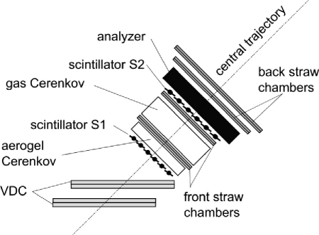
Figure 2: Schematic of the hadron arm detector package including the polarimeter.

In both HRS detector systems there are six scintillator paddles in plane S1 and six in S2. Each paddle is seen by one photomultiplier at each end. The paddles in both planes are oriented such that they are perpendicular to the spectrometer central ray. The distance between the two planes is 1.933 m on the electron side and 1.854 m on the hadron side. The active area of the S1 plane is 170 $\times$ 36 cm², and of the S2 plane 212$\times$60 cm². The thickness of each paddle in both planes is 0.5 cm. The scintillator paddles of both planes overlap by 0.5 cm to achieve complete coverage of the focal plane area.

The trigger for both spectrometers is similar and is formed from a coincidence between the signal from two scintillator planes, S1 and S2. The first requirement is to form a coincidence between the left and right signals from each paddle in the S1 and S2 planes. The time resolution per plane is about 0.3 ns (1$\sigma$). These coincidence signals are fed into a memory lookup unit (MLU) which is programmed to form a second trigger, called “S-Ray” (trigger T1 for electron HRS and trigger T3 for hadron HRS), by requiring that the paddles that fired in the S1- and S2 planes belong to an allowed hit pattern. The allowed hit pattern requires that if paddle $\mid$N$\mid$ is fired in the S1 plane, then in the scintillator plane S2 a signal must come from paddle $\mid$N-1$\mid$ or $\mid$N$\mid$ or $\mid$N+1$\mid$ or the overlap between two of those. Each spectrometer also has a “loose” trigger: for the electron arm it is formed by requiring that signals from two out of three detectors be present, S1-plane, S2- plane and the Čerenkov detector; the hadron arm loose trigger requires signals from just S1-plane and S2-plane. These loose triggers are used to obtain detector efficiencies. Finally, the S-ray trigger signals T1 and T3 form the “coincidence” trigger T5 for the experiment. These five different triggers, T1 to T5, are sent to the trigger supervisor (TS) and are also counted by scalers.

The TS was designed and built by the CEBAF online data acquisition (CODA) group. The functions of the TS include interface between the hardware trigger electronics and the computer data acquisition system, producing a computer busy signal that is used to calculate the computer dead-time, and pre-scaling of the trigger inputs T1 to T5.

The data acquisition system was entirely developed at JLab by the CODA groupcoda . In this experiment CODA was running on a single Hewlett-Packard (HP9000) computer. The two main tasks of CODA are to transmit information from the detectors to the computer via read out controllers (ROC) and build events by collecting data from all the ROCs. The data are stored on a hard disk temporarily for on-line analysis to monitor the experiment and then transfered to tapes in the JLab mass storage system to be used later for final off-line analysis.

II.1 Focal Plane Polarimeter

Polarization experiments have become increasingly important in the study of nuclear reactions. Focal plane polarimeters were standard equipment at intermediate energy proton accelerators, such as LAMPF lampf , TRIUMFtriumf , SATURNE saturne , and PSI psi . Experiments at these facilities have demonstrated the sensitivity of spin observables to small amplitudes. Similar considerations have more recently led to the development of proton polarimeters for use at electron accelerators, such as the MIT-Bates laboratory bates and at the Mainz Microtron mainz .

The FPP in Hall A at JLab was designed, built, installed and calibrated by a collaboration of Rutgers University, the College of William and Mary, Norfolk State University, the University of Georgia, and the University of Regina Mjones .

II.1.1 Physical Description of Focal Plane Polarimeter

The FPP is a part of the hadron detector package of the Hall A high resolution spectrometer. As shown in Fig. 2, the polarimeter is installed downstream from the focal plane VDCs; it is oriented along the mean particle direction in the focal plane area, at 45^∘ to the vertical. It consists of two front detectors to track incident protons, followed by a carbon analyzer and two rear detectors to track scattered particles.

The four tracking detectors of the FPP are drift chambers made of straw tubes; the straw tube design is based on the one used for the EVA detector at Brookhaven National Laboratory eva . The four drift chambers contain a total of 24 planes of straw tubes. Twelve of these are in the 2 front chambers CH1 and CH2, where they are oriented along the $u$ and $v$ directions at $+45^{\circ}$ and $-45^{\circ}$ relative to the spectrometer dispersive direction ($x$); each chamber has the configuration $vvvuuu$. In the back chambers CH3 and CH4 the configuration is $uuvvxx$ and $uuuvvv$, respectively, where $x$ indicates that the $x$-coordinate is measured, and the straws are oriented along the $y$ direction.

The individual straws are thin walled mylar tubes containing the anode wire at their center, and the gas mixture. They are made by wrapping an inner 10 $\mu$m thick aluminum foil, and two 50 $\mu$m thick mylar foils around a mandrel, together with a heat setting glue. The inner diameter of the straw is 10.44 mm. The ground connection to outside is made with silver epoxy to a brass ferrule inserted at both ends. As shown in Fig. 3, a delrin feed-through inserted in the ferrule provides gas feed and exhaust, and a positioning hole for a brass slit pin, into which the high voltage anode wire is soldered under prescribed stress to insure that the gravitational sagging and electrostatic deflection of the wire are small. The anode wire is gold plated 25 $\mu$m diameter tungsten-rhenium wire.

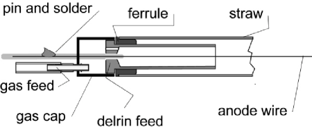
Figure 3: Schematic showing the end assembly of straw tubes.

The two front chambers are identical to one another and contain 1008 straw tubes each. In these two chambers the straw tubes are precisely spaced by inserting their ends into aluminum blocks in which holes of diameter 10.75 mm have been drilled with 10.95 mm spacing center-to-center. Each block has 3 layers of such holes separated vertically by 9.5 mm and shifted by half a hole separation, providing a very tight packing. Each block accommodates 16 straws in each of the 3 layers, for a total of 48. The spacing between the straws of each plane are maintained with mylar shims glued every 30 cm along the length. The active area for the front chambers is 60$\times$209 cm². The nominal distance between the two front chambers is 120 cm center to center; the intervening space was occupied during this experiment by the 100 cm gas Čerenkov detector: although not used in this experiment, it contributed an additional 3 mrad to the multiple scattering at the lowest proton energy.

The two back chambers contain a total of 3102 straws. Each chamber contains six planes of straws, with the successive layers of straws glued together using precision guiding plates and pins to insure accurate positioning, and is protected by 0.36 mm thick carbon fiber panels at the top and the bottom. Both chambers are positioned on a 1.9 cm thick and 31.5 cm wide plastic honeycomb, aluminum faced composite, that also provides a mounting surface for gas, high voltage distribution, and readout boards. Chambers CH3 and CH4 have active areas of 124 $\times$272 cm² and 142 $\times$295 cm², respectively. The distance between these two chambers is fixed and equal to 38.0 cm, center to center.

The gas mixture used in the FPP chambers is 62 %/38 % argon/ethane by volume. The straw chambers are operated at a high voltage of 1875 V. The drift velocity of electrons for this gas mixture and for this voltage is about 50 $\mu$m/ns over almost the entire volume of the tube. The efficiency of an individual straw tube for single track events is greater than 97 % after correction for the small gap between them.

The analyzer consists of five sets of graphite plates with different thicknesses. Each set is made of two halves that can be moved separately on left and right. The plates are beveled at an angle of 45^∘ so that the two halves overlap when closed. The plates have thicknesses of 1.9 cm, 3.8 cm, 7.6 cm, 15.2 cm and 22.9 cm and they are separated by $\sim$ 1.6 cm. The ability to vary the thickness of the analyzer is necessary to optimize the efficiency while maintaining the Coulomb multiple scattering angle within acceptable limits. The carbon thicknesses used in this experiment at different proton energies are given in Table I.

The main contribution to small angle multiple Coulomb scattering originates in the analyzer, with additional contributions from the scattering in the S2 paddles, the straw tubes in the two front chambers and the air between them. Table I gives typical multiple scattering angles for the relevant kinematics of this experiment. As Coulomb scattering is largely spin independent, in first order it does not affect the polarimeter performance; however, multiple scattering smears out the nuclear scattering distribution, and will therefore result in a small dependence of analyzing power upon the analyzer thickness. Coulomb scattering results in a strong forward peak of protons which did not undergo nuclear scattering; these events are suppressed by requiring a minimum scattering angle 2 to 3 times larger than the multiple scattering rms angle; here this minimum angle was fixed at 47 mrad (2.7^∘).

Table 1: Multiple scattering for the ten proton kinetic energies. ${T_{p}}_{inc.}$ is the incident proton kinetic energy, $C_{thick.}$ the analyzer thickness, $\vartheta^{rms}$ the root mean square Coulomb scattering angle, in FPP chambers (fpp), in the analyzer (C) and added quadratically (total).

${T_{p}}_{inc.}$	$C_{thick.}$	$\vartheta^{rms}_{fpp}$	$\vartheta^{rms}_{C}$	$\vartheta^{rms}_{total}$
(GeV)	(cm)	(mrad)	(mrad)	(mrad)
0.267	7.62	7.9	16.	17.8
0.426	22.86	5.9	20.8	21.6
0.639	41.91	3.8	18.1	18.5
0.799	41.91	3.1	16.1	16.4
0.959	49.53	2.8	14.8	15.1
1.014	49.53	2.7	13.1	13.4
1.156	49.53	2.2	11.6	11.8
1.333	49.53	2.1	10.4	10.6
1.599	49.53	1.8	9.3	9.5
1.865	49.53	1.6	8.2	8.4

To reduce the cost of electronics, the signal output of the individual straws is multiplexed in sets of eight. With multiplexing the maximum rate each tube can accept safely is 100 kHz. One end of each straw is connected to the high-voltage distribution board, and the other to a readout board. The Rutgers University electronics shop designed and built readout boards with 16 parallel channels. The input signal from each straw (typically 10 mV in size) is coupled to ground through a 1500 pF capacitor and fed into the input of an NEC1663 amplifier. The amplifier output, a 100 mV positive signal, is fed into a LeCroy MVL407 quad comparator. This is a leading edge discriminator that gives a logical true when the input signal exceeds a supplied positive threshold voltage. The output of the comparator is then fed into pulse shaping circuitry. The readout board is divided into two halves, each of eight channels. The shaping circuitry for the eight channels gives a different width logic pulse for each of the channels. This allows all eight to be multiplexed together with OR chips into a single output channel, reducing the number of cables and channels of TDC needed. To limit potential noise problems, ground planes are inserted within chamber readout card stacks, and differential output signals of amplitude 0.1 V are generated. Level shifter boards located away from the chambers, near the TDCs, convert these signals to usual ECL levels for input to the TDCs.

The output pulse widths for eight channels, generally adjusted to 1-2 % of the width, are given in Table II. The identification of a wire within a group of 8 is obtained by decoding the information from pipeline TDC’s which digitize both the leading and trailing edge times of the signal. The wire group is given by the multiplexed output carrying a signal; the actual position of the track requires decoding of the timing information to first identify the wire in the group and then calculate the drift time using drift velocity calibration data. Multiple tracks within the same subset of 8 wires cannot be decoded, unless the hits are separated by at least 250 ns.

Table 2: The output pulse widths for the eight channels of the multiplexing circuitry on the chamber read out cards.

Channel	1	2	3	4	5	6	7	8
Width (ns)	25	45	35	55	85-90	65	100-105	75

III DATA ANALYSIS

The data were analyzed with the standard Hall A analysis program called ESPACE espace . The output from ESPACE includes histograms, two-dimensional plots and multi-dimensional arrays (ntuples), which are used in further analysis to obtain quantities of interest, the $G_{Ep}/G_{Mp}$ ratio and the analyzing power $A_{y}$.

The kinematic settings of this experiment, the cuts applied in ESPACE, the selection of elastic events, the reconstruction of tracks in the FPP chambers, and the cuts on FPP variables are described in subsection A. A description of the azimuthal event distribution and asymmetry after scattering in the carbon analyzer, and spin transport through magnetic elements of the hadron HRS, is given in subsection B. The methods to calculate the $G_{Ep}/G_{Mp}$ ratio are described in subsection C, and subsection D describes the FPP calibration.

III.1 Kinematic Settings and Selection of Good Events

This experiment was performed at ten different values of $Q^{2}$; these $Q^{2}$ values as well as other useful kinematical quantities are given in Table III.

The Hall A analysis program ESPACE calculates the position and angle at the focal plane, $x^{fp},y^{fp},\theta^{fp},\phi^{fp}$, for each event from the raw VDC data. The position, angles and momentum for proton and electron at the target, $y,\theta,\phi,\delta$, are then calculated using the HRS optics matrix; $\delta$ is the relative momentum $\delta$=$\frac{p-p_{c}}{p_{c}}$, with $p$ and $p_{c}$ being the scattered particle’s momentum and the central momentum of the spectrometer, respectively.

Table 3: Beam energies and spectrometer settings of the experiment. $E_{beam}$ is the beam energy, $Q^{2}$ is the four momentum transferred square, ${p_{e}}_{c}$, ${\theta_{e}}_{c}$, ${p_{p}}_{c}$ and ${\theta_{p}}_{c}$ are central values of momentum and angle for the spectrometers detecting electrons and protons, respectively.

$E_{beam}$	$Q^{2}$	${p_{e}}_{c}$	${\theta_{e}}_{c}$	${p_{p}}_{c}$	${\theta_{p}}_{c}$
(GeV)	(GeV2)	(GeV/c)	(deg)	(GeV/c)	(deg)
0.934	0.50	0.675	52.59	0.756	45.28
0.934	0.80	0.516	79.81	0.991	30.84
1.821	1.20	1.193	43.45	1.268	40.36
3.592	1.50	2.815	22.11	1.463	46.52
3.592	1.80	2.656	25.01	1.649	42.92
4.087	1.90	3.093	22.28	1.712	43.35
4.087	2.17	2.950	24.40	1.872	40.68
4.091	2.50	2.774	27.08	2.068	37.68
4.091	3.00	2.507	31.29	2.357	33.59
4.087	3.50	2.241	35.90	2.642	29.87

The final optics matrix for each spectrometer was determined subsequent to this experiment using the procedure as described in Ref. nilanga . Figs. 4 and 5 show a comparison between the distributions of the target variables $y,\phi,\delta,\theta$ obtained from the data and calculated using the Monte Carlo program MCEEP mceep , for proton and electron at $Q^{2}$ of 3.5 GeV², respectively. The MCEEP results are normalized by a factor of about 0.85. This value seems quite reasonable, as in this experiment the trigger efficiency and the effect of boiling on target density were neither measured nor considered explicitly in the simulations. In addition, the BCM was not calibrated, as it would have been in the case of an absolute cross section measurement, for example. The agreement between the data and MCEEP results is good. Cuts were applied to all events for $\theta_{tar}$ ($\pm$65 mrad), $\phi_{tar}$ ($\pm$32 mrad), $y_{tar}$ ($\pm$6.5 cm) and $\delta$ ($\pm$5 %), to eliminate the events seen in the tails of Figs. 4 and 5.

Figure 4: Comparison between the target variables $y,\phi,\delta,\theta$ obtained from the data (dots) and calculated using the Monte Carlo program MCEEP (solid line) for protons detected in the right HRS. The MCEEP results are normalized by a factor of about 0.85, agreement between the data and the MCEEP results is good.

Figure 5: Comparison between the target variables $y,\phi,\delta,\theta$ obtained from the data (dots) and calculated using the Monte Carlo program MCEEP (solid line) for electrons detected in the left HRS. The MCEEP results are normalized by a factor of about 0.85, the agreement between the data and the MCEEP results is good.

The experimental event rates for each $Q^{2}$ and the one calculated with the Monte Carlo MCEEP are given in the Table IV. The actual event rates are always lower than the MCEEP rates by about 15 %, indicating that there is no significant background. The large difference seen between MCEEP and experimental event rate at $Q^{2}$ of 0.8 GeV² is due to a physical aperture cutting acceptance for the open collimator in the electron arm. Table IV also includes the total number of good events, average current, computer dead time, and average beam polarization value for each $Q^{2}$ value.

Table 4: Experimental conditions.

$Q^{2}$	Expt.	MCEEP	total no.	average	dead	average beam
	rate	rate	of events	current	time	polarization
(GeV2)	Hz	Hz		($\mu$A)	(%)
0.50	1050	1120	2.0 $\times$ 106	4	21	0.560$\pm 0.030$
0.80	250	420	4.6 $\times$ 106	10	1	0.544$\pm 0.006$
1.20	1100	1310	1.6 $\times$ 107	24	14	0.497$\pm 0.012$
1.50	420	480	9.2 $\times$ 106	10	4	0.483$\pm 0.021$
1.80	330	360	1.7 $\times$ 107	13	3	0.611$\pm 0.020$
1.90	1110	1160	5.6 $\times$ 107	63	24	0.391$\pm 0.002$
2.17	830	970	3.8 $\times$ 107	78	20	0.385$\pm 0.002$
2.50	540	650	5.6 $\times$ 107	74	4	0.390$\pm 0.008$
3.00	300	370	3.2 $\times$ 107	88	1	0.395$\pm 0.002$
3.50	140	160	2.0 $\times$ 107	94	1	0.384$\pm 0.007$

Selection of elastic $ep$ events was accomplished by implementing a correlated cut on the missing energy $E_{m}$ and missing momentum $p_{m}$. Due to the kinematic constraints of $ep$ elastic scattering, no further cuts were needed to remove background events. The missing energy $E_{m}$ is defined as:

$$E_{m}=E_{beam}+M_{p}-(E_{e}+E_{p})$$ (8)

where $E_{p}$ is the scattered proton energy, and $M_{p}$ is the mass of the proton. From conservation of momentum, the missing momentum, $P_{m}$, is defined as:

$$P_{m} = \sqrt{P_{m_{x}}^{2}+P_{m_{y}}^{2}+P_{m_{z}}^{2}}$$ (9)

$$P_{m_{x}} = p_{e}\cdot\sin\theta_{e}-p_{p}\cdot\sin\theta_{p}$$ (10)

$$P_{m_{y}} = p_{e}\cdot\sin\phi_{e}-p_{p}\cdot\sin\phi_{p}$$ (11)

$$P_{m_{z}} = P_{beam}-(p_{e}\cdot\cos\theta_{e}+p_{p}\cdot\cos\theta_{p})$$ (12)

where $p_{e}$ ($p_{p}$) is the scattered electron (proton) momentum, $\theta_{e}$ ($\theta_{p}$) is the scattered electron (proton) Cartesian angle in the horizontal plane, and $\phi_{e}$ ($\phi_{p}$) is the scattered electron (proton) Cartesian angle in the vertical plane. In Fig. 6, a histogram of the missing energy $E_{m}$ and missing momentum $P_{m}$ is shown. There is a peak at $E_{m}=0$ and a peak at about $P_{m}=10MeV/c$. The peak in the $P_{m}$ histogram is not centered at zero because $P_{m}$ is defined positive, and it has a larger width due to finite angular resolution in both the transverse ($\pm$2.0 mrad) and dispersive ($\pm$6.0 mrad) directions. A radiative tail is seen in the $E_{m}$ histogram up to about 125 MeV. The tail seen in the $P_{m}$ histogram includes the radiative tail as well as events that are multiple scattered in windows.

Figure 6: Histogram of the missing energy and momentum $E_{m}$ and $P_{m}$, respectively. The peaks at $E_{m}=0$ and at about $P_{m}$ = 10 MeV/c contain the elastic $ep$ events. The peak in $P_{m}$ has a larger width than $E_{m}$ because of finite angular resolution.

In Hall A, two methods of measuring the beam energy are now available, but at the time of this experiment neither was operational. The beam energy can be determined using the $ep$ elastic kinematics, either from the measured scattering angles of the electron and proton or from Eq. (8) by forcing $E_{m}=0$. Subsequent to this experiment, the beam energy was measured to a relative precision of about $1\times 10^{-3}$ and the central momentum of the spectrometer was determined to the same precision; using this central momentum of the spectrometer and Eq. (8), the beam energies were determined and are listed in Table III. Comparison to the beam energies determined from the scattering angles lead to the conservative conclusion that the beam energy was known with a relative precision of $2\times 10^{-3}$.

Once an event was identified as an elastic $ep$ scattering, the next step was to search for a good track in the front and back FPP drift tube chambers. The analysis part for the FPP was incorporated in the main ESPACE program by the FPP group Mjones ; this part of the program reconstructs position and angles, in the front and back FPP chambers, then calculates the polar and azimuthal scattering angles, $\vartheta$ and $\varphi$, respectively, and the position of the interaction point, $Z_{fpp}$, in the carbon analyzer. Tracking in the chambers is done in the $u$ and $v$ coordinates separately. Tracking starts with identifying clusters of hits in chambers CH1, CH2, CH3 and CH4. To determine a track for the front (back) chambers, there must be at least one hit in CH1 and CH2 (CH3 and CH4) and at least three hits total in the front (back) chambers. The efficiency for an individual straw to detect a proton is about 97 %; the total number of hits in the front chambers is usually about 5 or 6, and it is 4 or 5 for the rear chambers (as the X-plane is not used). The total number of possible front (back) tracks is the number of clusters in CH1 (CH3) times the number of clusters in CH2 (CH4). The straws have cylindrical symmetry so from a single hit it is impossible to distinguish if the proton passed to the left or right of the center wire (left/right ambiguity). For each possible track, a least-squares straight line fit is done for all possible combinations of left/right for each hit. Then, out of all possible tracks, the one with the smallest $\chi^{2}$ is selected as the good track. The only exception is when the track with the smallest $\chi^{2}$ has only three hits; then if there is another possible track with more hits, it is selected as the good track if its $\chi^{2}$ is reasonable.

The FPP chambers are aligned by using a software procedure. The carbon can be moved out to make a clear path between the front and back FPP chambers. Then the tracks in the front and back chambers are aligned to the tracks in the VDC so that the FPP has the same coordinate system as the VDC. This is done for each FPP chamber by adjusting the three positions: $z$ which is distance from the VDC and the zero of the $u$ and $v$ axes, and adjusting the three angles of the FPP chamber (angle of the $uz$ plane, angle of the $vz$ plane and the angle of the $uv$ plane). The actual alignment of the chambers was good, since in software the angles of the chambers are adjusted by less than a degree.

A good track in the front and back FPP chambers is required to determine the polar angle ($\vartheta$) and azimuthal angle ($\varphi$) of the scattered proton in the carbon analyzer. Next, we calculate the distance of closest approach between the tracks from the front chambers and the back chambers, and at what distance, $Z_{fpp}$, from the VDC the closest approach occurred. In Fig. 7, $Z_{fpp}$ is plotted for $Q^{2}$ = 3.5 GeV². The total thickness of carbon is 49.5 cm; it consists of 4 successive blocks which are separated by $\sim$ 1.6 cm, so one can see a peak for each block in Fig. 7. Chamber 3 is located at $Z_{fpp}$ of about 395 cm, as seen by the slight bump in Fig. 7 from scattering in this chamber. For a selection of good events, a cut is placed on $Z_{fpp}$ depending on the thickness of carbon used for the given proton momentum.

To reduce the false asymmetries a cone-test is applied for each event. An event passes the cone-test when the track that hit the back chambers at the measured polar angle would have hit the chambers for any possible azimuthal angle. In Fig. 8, the polar angle ($\vartheta$) is plotted versus $Z_{fpp}$ with the cone-test applied. As expected, the range of accepted polar angles increases as the interaction point in the carbon is closer to the back chambers.

Figure 7: Histogram of $Z_{fpp}$ for $Q^{2}$ = 3.5 GeV² with a total of 49.5 cm of carbon consisting of 4 successive blocks of carbon with thickness of 22.9, 15.2, 7.6 and 3.8 cm, indicated with different patterns.

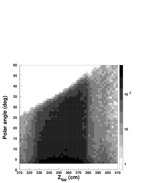
Figure 8: Plot of $Z_{fpp}$ versus the polar angle $\vartheta$ with the cone test applied.

III.2 Azimuthal Asymmetry, Spin Transport in HRS and Extraction of $G_{Ep}/G_{Mp}$

III.2.1 Azimuthal Asymmetry

Proton polarimeters are based on nuclear scattering from an analyzer material like carbon or polyethylene; the proton-nucleus spin-orbit interaction results in an azimuthal asymmetry in the scattering distribution which can be analyzed to obtain the proton polarization. The azimuthal angular distribution of the yield, $I$, of scattered protons is:

$$I~{}=~{}I_{o}~{}(1+A_{y}(\vartheta)\vec{P}^{fpp}\cdot\hat{n}),$$ (13)

where $I_{o}$ is the unpolarized yield, $\vec{P}^{fpp}$ is the proton polarization vector at the FPP, and $\hat{n}$ is a unit vector normal to the scattering plane defined as $\hat{n}=\hat{k}\times\hat{k}^{\prime}/\mid\hat{k}\times\hat{k}^{\prime}\mid$, with $\hat{k}$ and $\hat{k}^{\prime}$, the unit vectors in the direction of the incident and scattered proton, respectively; $A_{y}(\vartheta$) is the carbon analyzing power.

Fig. 9 shows a schematic of the polarimeter chambers and analyzer. It shows a non-central trajectory, where $\vartheta$ is the polar scattering angle, and $\varphi$ is the azimuthal scattering angle defined relative to the transverse direction in the polarimeter coordinate system.

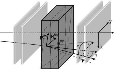
Figure 9: Schematic of the polarimeter chambers and analyzer, showing a non-central trajectory; $\vartheta$ is the polar angle, and $\varphi$ is the azimuthal angle from the $y$-direction counterclockwise.

The detection probability for a proton scattered by the analyzer with polar angle $\varphi$ and azimuthal angle $\varphi$ is given by:

$$f^{\pm}(\vartheta,\varphi)=\frac{\epsilon(\vartheta,\varphi)}{2\pi}\left(1\pm A_{y}(P_{t}^{fpp}\sin{\varphi}-P_{n}^{fpp}\cos{\varphi})\right)$$ (14)

where $\pm$ refers to the sign of the beam helicity, $P_{t}^{fpp}$ and $P_{n}^{fpp}$ are transverse and normal polarization components in the reaction plane at the analyzer, respectively; $P_{\ell}^{fpp}$ is not measured because it does not result in an asymmetry as seen in Eq. (13). In Eq. (14) the helicity-independent polarization has been omitted because the polarization from two-photon exchange contributions to elastic scattering is expected to be negligible. Here $\epsilon(\vartheta,\varphi)$ is an instrumental asymmetry that describes non-uniformities in detector response that might result from misalignments of the FPP chambers or from inhomogeneities in detector efficiency. The non-uniformity of $\epsilon(\vartheta,\varphi)$ depends upon the population of events on the detectors, which in turn is determined by the choice of kinematics. However, recognizing that the detector response is helicity independent and that non-uniformities are limited to a few percent, we may approximate Eq. (14) by,

$$f^{\pm}(\vartheta,\varphi)\approx\frac{1}{2\pi}\left(\epsilon(\vartheta,\varphi)\pm A_{y}(P_{t}^{fpp}\sin{\varphi}-P_{n}^{fpp}\cos{\varphi})\right)$$ (15)

and obtain

$$\epsilon(\vartheta,\varphi)\approx\pi\left(f^{+}(\vartheta,\varphi)+f^{-}(\vartheta,\varphi)\right)$$ (16)

The instrumental asymmetry can then be described well by the Fourier expansion

$$\epsilon(\vartheta,\varphi) = \alpha_{0}(\vartheta)+\alpha_{1}(\vartheta)\cos{\varphi}+\alpha_{2}(\vartheta)\cos{2\varphi}$$ (17)

$$+ \beta_{1}(\vartheta)\sin{\varphi}+\beta_{2}(\vartheta)\sin{2\varphi}+...$$

The angular dependence of the probability distribution $f^{\pm}$ is approximated by the normalized yields,

$$Y^{\pm}_{i}=\frac{1}{\Delta\varphi}\frac{N^{\pm}_{i}}{N_{in}^{\pm}\eta(\vartheta)}$$ (18)

where the index $i$ refers to a bin in $\varphi$, $\Delta\varphi$ is the width of the bin, $N^{\pm}_{i}$ is the number of events in bin $i$, $N_{in}^{\pm}$ is the number of protons with specified helicity incident upon the FPP, and $\eta(\vartheta)$ is the differential efficiency of the analyzing reaction, defined as the ratio of the number of protons scattered at angle $\vartheta$ with a good track in rear chambers over the number of incident protons with an acceptable track in the front chambers. It is also useful to define sum and difference histograms,

$$D_{i} = (Y^{+}_{i}-Y^{-}_{i})/2$$ (19)

$$E_{i} = (Y^{+}_{i}+Y^{-}_{i})/2$$ (20)

whose expectation values are given by,

$$\langle D_{i}\rangle = \frac{1}{2\pi}\left(A_{y}(P_{t}^{fpp}\sin{\varphi_{i}}-P_{n}^{fpp}\cos{\varphi_{i}})\right)$$ (21)

$$\langle E_{i}\rangle = \frac{\epsilon_{i}}{2\pi}$$ (22)

to lowest order in $\epsilon$. Thus, $E_{i}$ measures the efficiency while $D_{i}$ is sensitive to the transverse and normal components of the polarization at the FPP.

Figures 10 and 12 show the normalized yields and the sum and difference spectra for $Q^{2}=0.8$ and 3.5 GeV², respectively. Figures 11 and 13 show the efficiency spectra for the same $Q^{2}$ settings binned with respect to polar angle. Note that the widths of the scattering-angle bins were chosen to give approximately equal statistics.

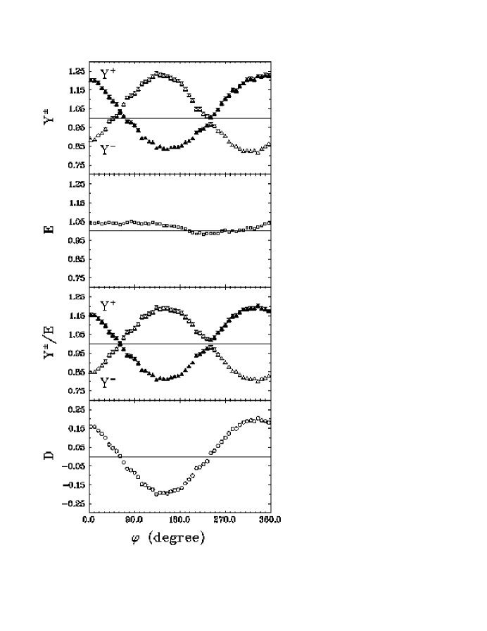
Figure 10: The azimuthal asymmetry distributions for $Q^{2}$=0.8 GeV². The first panel shows normalized yields $Y^{+}$ and $Y^{-}$, the second panel shows the sum distribution $E$, the third panel shows normalized yield $Y^{\pm}/E$ and the fourth panel shows the difference asymmetry spectrum $D$.

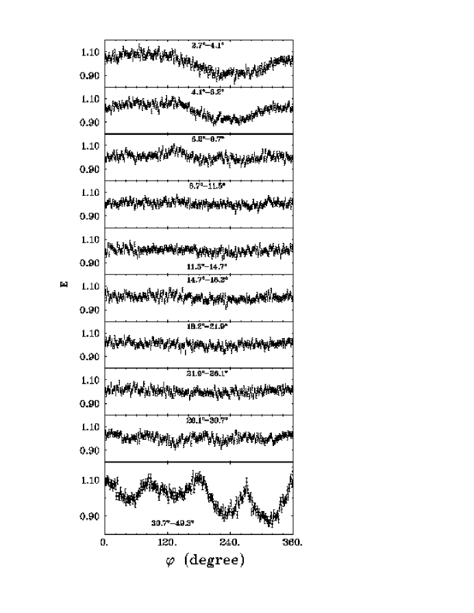
Figure 11: The sum $E=(Y^{+}+Y^{-})/2$ distributions for $Q^{2}$=0.8 GeV² for ten $\vartheta$ bins.

The first panel in Figs. 10 and 12 shows helicity-dependent normalized yields. In an ideal polarimeter these distributions would exhibit reflection symmetry about unity, but instrumental asymmetries perturb that ideal pattern, especially for the larger $Q^{2}$ where the physics asymmetry is smaller. The second panel in each of these figures shows instrumental asymmetries at the level of several percent. Figures 11 and 13 show these instrumental asymmetries divided into bins of the scattering angle $\vartheta$. The smooth instrumental asymmetry seen in Fig. 11 is clearly dominated by the lowest two $\vartheta$ bins, which are sensitive to chamber misalignment. This effect is stronger for the lowest $Q^{2}$ data. The experiment was performed in two periods separated by about six weeks with the five lower $Q^{2}$ point taken in the second period; no alignment data were taken at that time and the data show that the chambers must have been slightly misaligned in the intervening time. Nevertheless, the final results are not affected by this misalignment because it is helicity independent and therefore cancels when the difference between the two helicity states is calculated. The efficiency spectrum for $Q^{2}=3.5$ GeV² contains higher frequency components arising primarily from large scattering angles, as shown in the bottom panel of Fig. 13, that arise from edge effects. These effects do not affect the final results either because they are helicity independent also. Furthermore, omission of the large $\vartheta$ bin simply increases the statistical uncertainty in recoil polarization by about 5 % (relative) without altering the reported results.

Figure 12: The azimuthal asymmetry distributions for $Q^{2}$=3.5 GeV². The first panel shows normalized yields $Y^{+}$ and $Y^{-}$, the second panel shows the sum distribution $E$, third panel shows normalized yield $Y^{\pm}/E$ and the fourth panel shows the difference asymmetry spectrum $D$ together with sinusoidal fits and $\chi^{2}$ values for each curve.

The third panel in Figs. 10 and 12 shows normalized yields corrected for instrumental asymmetry, namely $Y^{\pm}/E_{i}$. These spectra show the reflection symmetry expected for an ideal polarimeter. Finally, the bottom panel of these figures shows the asymmetry spectra together with sinusoidal fits in Fig. 12 that can be described by:

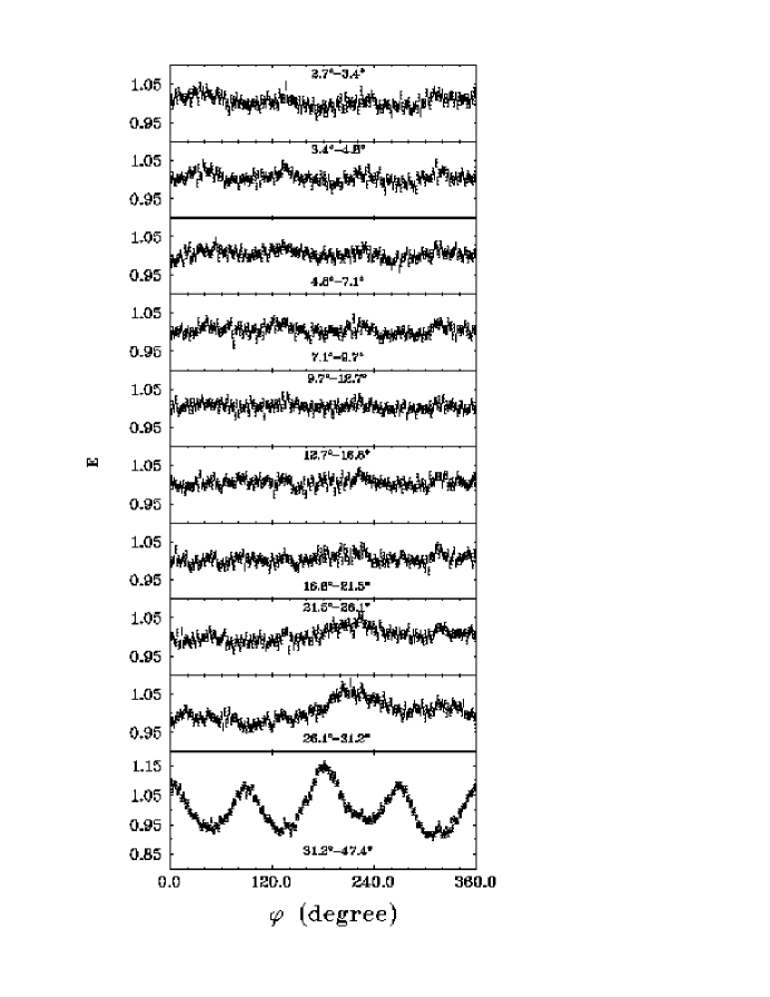
Figure 13: The sum $E_{i}=(Y^{+}+Y^{-})/2$ distributions for $Q^{2}$=3.5 GeV² for ten $\vartheta$ bins.

$$D_{i}=D_{0}\cos{(\varphi+\delta)}$$ (23)

where the phase shift $\delta$ would be proportional to $\mu_{p}G_{Ep}/G_{Mp}$ in an ideal spectrometer. For the final analysis spin precession in the spectrometer was handled event-by-event using the procedures to be described in subsequent sections. For the present purposes it is sufficient to observe that pure sinusoids fit the difference spectra with reduced $\chi^{2}$ better than unity, showing that the instrumental asymmetries have been eliminated. Therefore, analysis of the difference spectrum is insensitive to instrumental asymmetry.

To demonstrate helicity independence at the focal plane, we show the ratio of helicity plus to minus events at $Q^{2}$ of 3.5 GeV² for variables $x^{fp},y^{fp},\theta^{fp}$, and $\phi^{fp}$ in Fig. 14; the ratio is equal to one within statistical uncertainty (note the expanded y-scale) and is constant for each one of the four focal plane variables, thus indicating that there is no helicity dependence between $N^{+}$ and $N^{-}$ events in the focal plane of the hadron spectrometer.

Figure 14: The ratio $N^{+}$/$N^{-}$ at $Q^{2}$ of 3.5 GeV²; the ratio is close to one and constant for each one of the four focal plane variables, thus indicating that there is no helicity dependence of $N^{+}$ and $N^{-}$ events in the focal plane.

III.2.2 Spin Transport in HRS

The proton spin precesses as it travels from the target to the focal plane through the magnetic elements of the HRS as shown in Fig. 15, and therefore the polarization components at the target and at the FPP are different. The hadron HRS in Hall A consists of 3 quadrupoles and one dipole with shaped entrance and exit edges, as well as a radial field gradient.

The primary precession angle, $\chi_{\theta}$, in Fig. 15 is defined as the difference between the spin and the trajectory rotation angles in the dispersive direction and can be expressed as:

$$\chi_{\theta}=\gamma(\mu_{p}-1)(\theta_{B}+\theta-\theta^{fp}),$$ (24)

where $\gamma$ is $E_{p}/M_{p}$, $\mu_{p}$ is the proton magnetic moment, ($\theta_{B}+\theta-\theta^{fp}$) is the bending angle in the dipole for a given event; $\theta^{fp}$ is the angle at focal plane, $\theta$ is the angle at the target, and in the HRS $\theta_{B}$ = 45^∘ for the central trajectory. As shown in Fig. 15, in first approximation for the homogeneous dipole field, the transverse polarization component $P_{t}$ is parallel to the field and does not precess; the longitudinal polarization component is perpendicular to the field and precesses with an angle $\chi_{\theta}$.

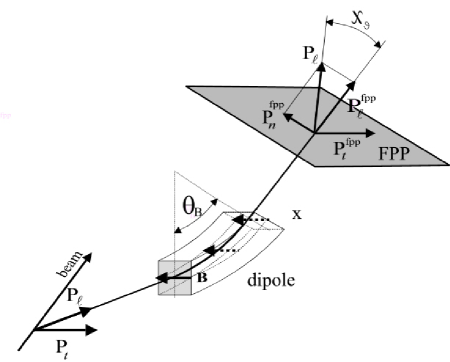
Figure 15: Schematic drawing showing the precession by angle $\chi_{\theta}$ of the $P_{\ell}$ component of the polarization in the dipole of the HRS.

For the HRS, the polarization vectors at the polarimeter, $\vec{P}^{fpp}$, are related to those at the target, $h\vec{P}$, where $\vec{P}$ is the polarization as given by Eqs.  (3), (4), and (5) through a 3-dimensional rotation matrix, $(\bf S)$, as follows:

$\left(\begin{array}[]{c}P_{n}^{fpp}\\ P_{t}^{fpp}\\ P_{\ell}^{fpp}\end{array}\right)=\left(\begin{array}[]{ccc}S_{nn}&S_{nt}&S_{n\ell}\\ S_{tn}&S_{tt}&S_{t\ell}\\ S_{\ell n}&S_{\ell t}&S_{\ell\ell}\end{array}\right)\left(\begin{array}[]{c}P^{ind}_{n}\\ hP_{t}\\ hP_{\ell}\end{array}\right)$.

where $h$ is the electron beam helicity, understood here to be the value of the longitudinal beam polarization component at the target, described with sign and magnitude. Each one of the 9 matrix elements depends upon a particle’s trajectory in the spectrometer, and therefore upon the 4 reconstructed kinematical variables $y,\phi,\delta\mbox{ and }\theta$ of the recoil proton at the target. In the case of elastic $ep$ scattering, there is no helicity dependent polarization component $P_{n}$ at the target in the single-photon exchange approximation, however the helicity independent component $P^{ind}_{n}$ may be induced due to the two-photon exchange mechanism, but this component is very small. The two polarization transfer components $P_{n}^{fpp}$ and $P_{t}^{fpp}$ in Eq. (14) for each event, are then given by INPC98 :

$$P_{n}^{fpp} = S_{nt}hP_{t}+S_{n\ell}hP_{\ell}~{}~{}~{}~{}\mbox{ and}$$

$$P_{t}^{fpp} = S_{tt}hP_{t}+S_{t\ell}hP_{\ell}.$$ (25)

With the assumption that there is only a dipole with an homogeneous field in front of the FPP, then $S_{tt}=1$, $S_{n\ell}=\sin\chi_{\theta}$, $S_{t\ell}=S_{nt}=0$, and Eq. (25) simplifies to:

$$P_{t}^{fpp}=~{}hP_{t}\mbox{ and }P_{n}^{fpp}=~{}hP_{\ell}~{}\sin\chi_{\theta}.$$ (26)

However, the homogeneous dipole model is not appropriate for the HRS, as it does not take into account the precession in the non-dispersive direction due to quadrupoles, fringe fields, and radial field gradient in the dipole.

A better approximation is to calculate the spin matrix elements $S_{ij}$ from the bend angles in the spectrometer, with several less restrictive assumptions about the magnetic field configuration, (i) the longitudinal component of the magnetic field with respect to the particle trajectory can be neglected, and (ii) the trajectory angles in the dipole change linearly along the path length tnote . The $S_{ij}$ elements under these assumptions are:

$$S_{nt} =- \sin\chi_{\theta}~{}\sin\chi_{\phi}~{}\cos\chi_{\phi}^{\prime}+O(\chi_{\phi}\times\chi_{\phi}^{\prime})$$

$$S_{n\ell} = \sin\chi_{\theta}~{}\cos\chi_{\phi}$$

$$S_{tt} = \cos\chi_{\phi}~{}\cos\chi_{\phi}^{\prime}$$

$$S_{t\ell} = \sin\chi_{\phi},$$ (27)

where the angles

$$\chi_{\phi} = \gamma(\mu_{p}-1)[-(\phi-\phi^{fp})+(\phi^{d}-\phi^{fp})(1-\cos\chi_{\theta})$$

$$- \Delta\phi^{d}\left(1-\frac{2\sin\chi_{\theta}}{\chi_{\theta}}+\cos\chi_{\theta}\right)]$$

$$\chi_{\phi}^{\prime} = \gamma(\mu_{p}-1)[-(\phi^{d}-\phi^{fp})\sin\chi_{\theta}$$ (28)

$$+ \Delta\phi^{d}\left(\frac{2(1-\cos\chi_{\theta})}{\chi_{\theta}}-\sin\chi_{\theta}\right)]$$

represent the precession in the non-dispersive direction. Here $\phi-\phi^{fp}$ is the corresponding trajectory total bending angle; $\phi^{d}$ is the mean angle in the dipole, and $\Delta\phi^{d}$ is half of the bending angle in the dipole in the non-dispersive plane. In first order the later two angles depend only on the non-dispersive target coordinate and angle:

$$\phi^{d} = (\phi^{d}|y)y+(\phi^{d}|\phi)\phi$$

$$\Delta\phi^{d} = (\Delta\phi^{d}|y)y+(\Delta\phi^{d}|\phi)\phi$$ (29)

The parameters, $(\phi^{d}|y)$, $(\phi^{d}|\phi)$, $(\Delta\phi^{d}|y)$, and $(\Delta\phi^{d}|\phi)$ are the couplings to the non-dispersive coordinate and angle at the target, and cannot be measured directly; however they can be fitted and obtained from the data without using any spectrometer model. An analysis in tnote also shows that for the HRS, because of the relatively small angular acceptance and weak fringe field effects, both being sources of the longitudinal field component, assumption (i) above is fulfilled with good accuracy. Comparison with the full COSY calculation described below, shows that assumption (ii) is also a good approximation (see part IV C).

The results presented here were obtained with spin matrix elements $S_{ij}$ calculated using a model of the HRS with quadrupoles, fringe fields, and radial field gradient in the dipole, for each tuning of the spectrometer and event by event with the differential-algebra-based transport code COSY bertz . For a given central momentum, the output of the COSY code is a table of the expansion coefficients $C_{ij}^{klmnp}$ of the rotation matrix. The matrix elements are calculated for each event using the $x$, $\theta$, $y$, $\phi$, and $\delta$ coordinates of the individual protons at the target with the form:

$$S_{ij}=\sum_{k,l,m,n,p}C_{ij}^{klmnp}x^{k}\theta^{\ell}y^{m}\phi^{n}\delta^{p}.$$ (30)

The contribution to the systematic uncertainty due to the model parameters will be discussed in part IV C.

III.3 Extraction of Ratio $G_{Ep}/G_{Mp}$

Results of this experiment published previously jones were obtained using the analysis method of Ref. INPC98 , we will call this the “old method”. The data presented here result from a complete re-analysis following a “new method”. In Appendix A, both methods are described in some detail.

In both methods, the new and the old, the FPP data were analyzed in bins of polar scattering angle $\vartheta$, such that statistics are approximately the same in all bins. The analyzing power $A_{y}$ appearing in formulas in the Appendix A and in this section is an average analyzing power in each $\vartheta$ bin. The ratio $G_{Ep}/G_{Mp}$ was extracted for each bin and the ratio for a given $Q^{2}$ is the average over all $\vartheta$-bins.

With the old method one calculates first the average asymmetries at the focal plane and then transports them to the target using the average spin matrix elements, as discussed in Appendix A 1. Assuming that the detector efficiency $\epsilon(\varphi)$ is a constant, and because the azimuthal scattering angle $\varphi$ in the analyzer is independent of the target quantities $x$, $\theta$, $y$, $\phi$ and $\delta$, Eqs. (53) and (54) from Appendix A 1 can be written simply as:

$$\overline{A_{y}P_{n}^{fpp}}=hA_{y}P_{t}\overline{S_{nt}}+hA_{y}P_{\ell}\overline{S_{n\ell}}$$

$$\overline{A_{y}P_{t}^{fpp}}=hA_{y}P_{t}\overline{S_{tt}}+hA_{y}P_{\ell}\overline{S_{t\ell}},$$ (31)

where $\overline{{A_{y}P_{t}^{fpp}}}$ and $\overline{{A_{y}P_{n}^{fpp}}}$ are the effective asymmetries measured at the focal plane, and $\overline{S_{ij}}$ are the mean values of the spin matrix elements; they are averages over the kinematical acceptance of the experiment. These linear equations must be inverted to obtain the target polarization asymmetries $hA_{y}P_{\ell}$ and $hA_{y}P_{t}$, which requires the determinant of the averaged spin transfer coefficients, shown below:

$$\begin{array}[]{c}\left|\begin{array}[]{cc}{\overline{S_{nt}}{}{}}&\overline{S_{n\ell}}\\ \overline{S_{tt}}{}{}&\overline{S_{t\ell}}\end{array}\right|.\end{array}$$ (35)

When the precession angle $\chi_{\theta}$ is close to 180^∘, the determinant is close to zero as the matrix element $S_{n\ell}~{}=~{}\sin\chi_{\theta}~{}\cos\chi_{\phi}$, and the spin transfer coefficients $S_{nt}$ and $S_{t\ell}$ are very small; hence the calculation of the polarization components at the target is less accurate; this occurs for $Q^{2}$ of 1.8, 1.9, 2.5 GeV² and more so for $Q^{2}$ of 2.17 GeV².

To overcome the difficulty associated with $\chi_{\theta}$ near $180^{0}$, a new method was developed to analyze the data; this method calculates the mean values of the asymmetries at the target rather than at the focal plane, as described in Appendix A 2. Assuming, again for simplicity, that the efficiency $\epsilon(\varphi)$ is constant, the determinant for the set of equations (57, 58) obtained with the new method in Appendix A 2, is:

$$\begin{array}[]{c}\left|\begin{array}[]{cc}\overline{S_{nt}S_{n\ell}}+\overline{S_{tt}S_{t\ell}}&\overline{S_{n\ell}^{2}}+\overline{S_{t\ell}^{2}}\\ \overline{S_{nt}^{2}}+\overline{S_{tt}^{2}}&\overline{S_{nt}S_{n\ell}}+\overline{S_{tt}S_{t\ell}}\end{array}\right|\end{array}$$ (39)

Now the determinant is non-zero even when $\overline{S_{n\ell}}$=0, because $\overline{S_{n\ell}^{2}}\neq$0, even if $\overline{\chi_{\theta}}\simeq 180^{0}$.

Both methods give very similar results, except for the region of $\chi_{\theta}\approx 180^{0}$, where the old method gives larger uncertainties, and a slightly different result but still within the statistical uncertainty at the $Q^{2}$ of 1.8, 1.9 and 2.5 GeV². With the new method it became possible to obtain a ratio value at $Q^{2}$ = 2.17 GeV², which has $\overline{\chi_{\theta}}=180^{0}$ for the central proton momentum.

The values of the two asymmetries at the target, $hA_{y}P_{t}$ and $hA_{y}P_{\ell}$, obtained as discussed above, can now be used to calculate the ratio $G_{Ep}/G_{Mp}$ as shown below:

$$\frac{G_{Ep}}{G_{Mp}}=-\frac{hA_{y}P_{t}}{hA_{y}P_{\ell}}\frac{(E_{e}+E_{e^{\prime}})}{2M}\tan\frac{\theta_{e}}{2}$$ (40)

As can be seen from this equation, neither the beam polarization nor the polarimeter analyzing power need to be known to extract the ratio, which results in very small systematic uncertainties.

III.4 FPP Calibration

Elastic $\vec{e}p\rightarrow e\vec{p}$ scattering provides a method to measure the analyzing power of the analyzer and therefore calibrate the FPP. After having obtained the ratio $G_{Ep}/G_{Mp}$ in a given kinematics following the method described in section III C, the values of the polarization observables at the target can be calculated from Eqs. (4, 5) rewritten as:

$$P_{t} = -2\sqrt{\tau(1+\tau)}\frac{(G_{Ep}/G_{Mp})\tan\frac{\theta_{e}}{2}}{(G_{Ep}^{2}/G_{Mp}^{2}+\tau/\epsilon)}$$ (41)

$$P_{\ell} = \frac{E_{beam}+E_{e}}{M_{p}}\sqrt{\tau(1+\tau)}\frac{\tan^{2}\frac{\theta_{e}}{2}}{(G_{Ep}^{2}/G_{Mp}^{2}+\tau/\epsilon)}$$ (42)

These are values of $P_{t}$ and $P_{\ell}$ at the target, averaged over the acceptance of the detectors. The asymmetry values $hA_{y}P_{t}$ and $hA_{y}P_{\ell}$ obtained from Eqs. (57, 58) in Appendix A 2, are then used to obtain the analyzing power. For each proton energy, the average value of the beam helicity, $h$ from Table IV, was used to obtain the analyzing power $A_{y}$.

The important properties of the FPP are the analyzing power $A_{y}(\vartheta)$ and the efficiency of the analyzing reaction, $\eta(\vartheta)$. The analyzing power $A_{y}(\vartheta)$ is plotted as filled triangles in Fig. 16 versus the polar scattering angle $\vartheta$ at the ten proton energies of this experiment; for proton energies 0.879 and 0.934 GeV the data have been placed in the same panel, as filled triangle and circle, respectively.

Figure 16: Analyzing power as a function of polar scattering angle $\vartheta$ in FPP, for the JLab Hall A polarimeter (filled triangle and circle); also shown are fits as solid line and data from other earlier calibration experiments as open squares.

In each panel the energy is that of the proton corrected for energy loss to half the thickness of the C-analyzer given in Table V. For comparison with the world data, fits adapted to the actual thickness of the analyzer used in this experiment are shown. At the two lowest proton energies the fits are from the calibration of Waters et al. triumf , and in the next two they are from the calibration of Ransome et al. lampf . All others are from the 14 parameter fit of the Saclay calibration of Cheung et al. saturne . In the same figure we also show as open squares data from various sources when available; in panel one the data at 0.225 GeV are from Ref. psi , in panels two and three the data at 0.440 and 0.691 GeV are from Ref. lampf , and in panels for 1.045 GeV to 1.795 GeV, the data are from Ref. saturne . One must take notice that all earlier data were taken with significantly thinner C-analyzers. Overall the new data are in good agreement with fits and with previous data when available.

The efficiency $\eta(\vartheta)$ for the ten values of $Q^{2}$ is shown in Fig. 17. For the 6 panels with the larger energies, the $\vartheta$ dependence is very much the same, as expected because the thickness of the C-analyzer was a constant 49.53 cm (see Table I). A cut was applied to eliminate all data below 2.7^∘ and above 50.0^∘. The lower cut was defined by the Coulomb scattering and the resolution of the drift chambers; the upper cut is determined by the size of the FPP back chambers. We include events with smaller and with larger scattering angles than in Ref. saturne because we used drift chambers instead of the multi wire proportional chambers used in the calibration of Bonin et al. and Cheung et al., and have therefore better position and angular resolution, and also we used larger rear chambers. The enhancement seen at small angles is indicative of Coulomb scattering events from protons without nuclear interaction and with scattering angles larger than 2.7^∘. Also as expected, the width of the forward peak is seen to decrease with increasing T_p.

Figure 17: Differential efficiency as a function of proton kinetic energy, ${T_{p}}_{analy.}$, evaluated at the half thickness of the analyzer.

Combining the $A_{y}(\vartheta)$ from Fig. 16 and $\eta(\vartheta)$ of Fig. 17 gives the differential figure of merit (FOM) $\eta(\vartheta)A_{y}^{2}(\vartheta)$. The FOM values allow a quick evaluation of the number of “good” incident protons required to obtain a given statistical uncertainty in the polarization components. The calibration data for analyzing power $A_{y}$, efficiency $\eta$, and FOM are given in Table V.

Table 5: Averaged analyzing power, $\overline{A}_{y}$, and integrated efficiency $\eta_{int.}$ and figure of merit, FOM, of the FPP for the ten proton kinetic energies of the experiment, ${T_{p}}_{analy.}$. The range of integration for all three quantities is $2.7^{\circ}<\vartheta<50^{\circ}$. Both the statistical (stat.) and systematic (sys.) uncertainties for ${FOM}$ are given.

${T_{p}}_{analy.}$	$\overline{A}_{y}\pm stat$	$\eta_{int.}$	${FOM}\pm stat.\pm sys.$
(GeV)	(cm)		$\times 10^{-2}$
0.244	0.274 $\pm$ 0.006	0.115	1.32 $\pm$ 0.04 $\pm$ 0.08
0.375	0.223 $\pm$ 0.002	0.244	1.57 $\pm$ 0.02 $\pm$ 0.10
0.561	0.183 $\pm$ 0.002	0.298	1.13 $\pm$ 0.02 $\pm$ 0.07
0.715	0.195 $\pm$ 0.005	0.323	1.25 $\pm$ 0.05 $\pm$ 0.09
0.879	0.162 $\pm$ 0.004	0.358	0.98 $\pm$ 0.03 $\pm$ 0.09
0.934	0.156 $\pm$ 0.004	0.362	0.94 $\pm$ 0.03 $\pm$ 0.09
1.045	0.145 $\pm$ 0.008	0.382	0.83 $\pm$ 0.06 $\pm$ 0.05
1.258	0.124 $\pm$ 0.003	0.401	0.65 $\pm$ 0.02 $\pm$ 0.06
1.528	0.099 $\pm$ 0.002	0.425	0.50 $\pm$ 0.01 $\pm$ 0.04
1.795	0.080 $\pm$ 0.002	0.443	0.35 $\pm$ 0.01 $\pm$ 0.03

The statistical uncertainty in the results of this experiment is directly dependent on the analyzing power $A_{y}$ and the differential efficiency $\eta$, and can be written as:

$$\Delta P_{n}^{fpp}=\Delta P_{t}^{fpp}=\sqrt{\frac{2}{\eta A_{y}^{2}(N_{tot})}}=\sqrt{\frac{2}{FOM(N_{tot})}}$$ (43)

where $N_{tot}=N_{in}^{+}~{}+~{}N_{in}^{-}$ is the total number of incident protons on the analyzer.

IV RESULTS AND DISCUSSION

IV.1 Experimental Results

Figure 18 shows the results for the ratio $\mu_{p}G_{Ep}/G_{Mp}$ from this experiment as filled circles, and from all experiments that took place after 1970 with same symbols as in Fig. 1. Our data points are shown with statistical uncertainties only; the systematic uncertainties are indicated by the black polygon. The data are tabulated in Table VI, where statistical and systematic uncertainties, as well as $Q^{2}$ bin sizes are given for each data point. The results from this experiment differ from those previously published jones in three ways: the points at 1.77, 1.88 and 2.47 GeV² have moved slightly as a result of the new analysis method described in subsection III C and Appendix A, a new point was obtained at Q²=2.13 GeV², and the systematic uncertainties are 2-3 times smaller.

Figure 18: The ratio $\mu_{p}G_{Ep}/G_{Mp}$ from this experiment, filled circles, compared to world data, shown with the same symbols as in Fig. 1, with the 2 data points of Ref. milbrath shown with filled squares. The absolute value of systematic errors from this experiment is shown by the shaded polygon.

Table 6: The ratio $\mu_{p}G_{Ep}/G_{Mp}\pm$ statistical uncertainty (1$\sigma$). $\Delta_{sys}$ is the systematic uncertainty from Table VII. $\overline{Q}^{2}$ and $\overline{\chi}_{\theta}$ are the weighted average four momentum transfer squared and spin precession angle, respectively. $\Delta Q^{2}$ is half the $Q^{2}$ acceptance. The last column $P_{t}/P_{\ell}$ is the ratio of measured polarization components at the target, the relative uncertainty is the same as for $\mu_{p}G_{Ep}/G_{Mp}$.

$\overline{Q}^{2}\pm\Delta Q^{2}$	$\overline{\chi}_{\theta}$	$\mu_{p}G_{Ep}/G_{Mp}$	$\Delta_{sys}$	$P_{t}/P_{\ell}$
(GeV2)	(deg)	($\pm$ stat. uncert.)
0.49$\pm$.04	105	0.979 $\pm$ 0.016	0.006	-0.822
0.79$\pm$.02	118	0.951 $\pm$ 0.012	0.010	-0.527
1.18$\pm$.07	136	0.883 $\pm$ 0.013	0.018	-0.492
1.48$\pm$.11	150	0.798 $\pm$ 0.029	0.026	-0.422
1.77$\pm$.12	164	0.789 $\pm$ 0.024	0.035	-0.381
1.88$\pm$.13	168	0.777 $\pm$ 0.024	0.033	-0.368
2.13$\pm$.15	181	0.747 $\pm$ 0.032	0.034	-0.329
2.47$\pm$.17	196	0.703 $\pm$ 0.023	0.033	-0.284
2.97$\pm$.20	218	0.615 $\pm$ 0.029	0.021	-0.224
3.47$\pm$.20	239	0.606 $\pm$ 0.042	0.014	-0.198

Figure 19: The ratio $\mu_{p}G_{Ep}/G_{Mp}$ obtained in this experiment, and other polarization transfer experiments, including milbrath ; pospischil ; gayou ; gayou2 . The curves are fits to the Rosenbluth separation data: one from Bosted bosted2 shown as dotted line, and two from rosenblut shown as solid line for all world data, and a dashed line for a selected subset of the world data.

As seen in Fig. 18, the electric form factor data from the past 30 or so years can be described by the dipole form factor, $G_{Ep}/G_{D}\approx 1$ considering the spread in the data from different experiments; however, the data from this experiment deviate from the dipole form factor significantly starting at $Q^{2}$ of 1 GeV². Note that the results from this experiment are in apparent good agreement with the earlier data of Refs. berger ; price ; bartel which have much larger uncertainties; also considering the larger uncertainties, the SLAC data of Ref. andivahis are compatible with our results up to about $Q^{2}$ of 2.5 GeV².

Several global analyses of the $\mu_{p}G_{Ep}/G_{Mp}$ ratio obtained by Rosenbluth separation method have been done. We show in Fig. 19 three of these fits: the dotted line is the Bosted fit bosted2 . The solid and dashed lines are from a recent global fit by Arrington rosenblut , including all existing data, and a subset of the data, respectively. The subset of the data is a biased selection which was chosen to give the lowest possible ratio and therefore represents a lower limit for the ratio extracted from the cross section data alone. All fits tend to be dominated by the more recent SLAC data. Only the $\mu_{p}G_{Ep}/G_{Mp}$ ratios obtained by recoil polarization are shown here; the data from this paper, from ref. gayou , the early data of Milbrath et al. milbrath , Pospischil et al. pospischil , and a collection of measurements made in various Hall A experiments and analyzed by Gayou et al.gayou2 . We conclude from the comparison between Rosenbluth and polarization data shown in Fig. 19 and from the further analysis done in ref. rosenblut , that the two methods give definitively different results; the difference cannot be bridged by either simple re-normalization of the Rosenbluth data or by variation of the polarization data within the quoted statistical and systematic uncertainties.

The new results are the first high precision measurements of the ratio $G_{Ep}/G_{Mp}$ above $Q^{2}$ of 1.0 GeV². The result for the ratio shows a systematic decrease as $Q^{2}$ increases from 0.5 GeV² to 3.5 GeV², which indicates that $G_{Ep}$ falls faster than $G_{Mp}$. In the non-relativistic limit, this fact could be interpreted as indicating that the spatial distributions of charge and magnetization currents in the proton are definitely different.

IV.2 Nature of the Data

To illustrate the stability of the polarization data presented in the previous part, we show in Fig. 20 the variation of the the polarization component ratio, $P_{t}/P_{\ell}$ at the target, as a function of the four target variables: $y,~{}\phi,~{}\delta~{}$ and $\theta$, for $Q^{2}$=3.5 GeV². In each one of the panels, the data are integrated over the full experimental acceptance for the other three variables; therefore the statistics in each panel are not independent. The filled circles are the results obtained with full COSY calculation; the open triangles are the values obtained not taking into account the spin rotation due to the quadrupoles and the field gradient and fringe field of the dipole. The scatter in the data (filled circles) for each variable is compatible with the statistical uncertainty on $P_{t}/P_{\ell}$, which are shown as the dashed lines below and above the average, shown as the solid line; a constant value of $P_{t}/P_{\ell}$ over the acceptance of the spectrometer in each one of the four target variables demonstrates that the spin transport matrix elements are correct over the whole acceptance of the spectrometer, and indirectly, that the spectrometer model used in COSY is correct. The values of $P_{t}/P_{\ell}$ are given in Table VI.

Figure 20: The ratio $P_{t}/P_{\ell}$ at the target, plotted as a function of the 4 kinematical target variables for Q²=3.5 GeV². The filled circles are the results from COSY; the open triangles are the values obtained not taking into account the spin rotation due to the quadrupoles and the field gradient and fringe field of the dipole. Also shown is the range of statistical uncertainty corresponding to the uncertainty on $\mu_{p}G_{Ep}/G_{Mp}$.

The systematic decrease of the ratio $\mu_{p}G_{Ep}/G_{Mp}$ shown in Fig. 18 and given in Table VI can be traced to the observed absolute values of $P_{t}$ being systematically and increasingly smaller than the values calculated using the dipole form factor $G_{D}=(1+Q^{2}/0.71)^{-2}$, and $G_{Ep}/G_{D}$ and $G_{Mp}/\mu_{p}G_{D}$. This is demonstrated in Fig. 21, where the values of $P_{t}$ at the target obtained in this experiment are shown versus Q² as solid circles. Also shown in this figure are the values of $P_{t}$ calculated from Eqs. (4) and (5) with dipole form factors as open triangles, and open circles are $P^{fpp}_{t}$ calculated from the data. It is seen from this figure that the additional polarization rotation introduced by the quadrupoles, and fringe and indexed fields in the dipole, is always small, and tend to decrease the magnitude of $P^{fpp}_{t}$ from its value at the target. The spin transport coefficient in Eq. 31 $\overline{S}_{t\ell}$ is small but not zero; it would average to zero over a symmetric angular distribution of events in the HRS acceptance. However, the $Q^{2}$ dependence of the cross section results in more events at small scattering angle than large, and that results in a non-zero average value of $S_{t\ell}$, producing the small change of the observed transverse component at the target seen in Fig. 21. Noticeable is the abrupt bend for all three sets; this apparent discontinuity is the result of the choice of beam energies: the last five points were taken at constant beam energy, whereas the first five where taken with an increasing energy to optimize the experiment.

Figure 21: The transverse component of the polarization at the target, $P_{t}$ measured in this experiment is shown as solid circles. The open triangles show the value of $P_{t}$ calculated using the dipole approximation, or scaling assumption: $G_{E}=G_{D}$ and $G_{M}=\mu_{p}G_{D}$. Also shown as open circles are the values of $P_{t}$ from the approximation $P_{t}=P_{t}^{fpp}$, not taking into account the spin rotation due to the quadrupoles and the field gradient and fringe field of the dipole.

IV.3 Discussion of Systematic uncertainties

The two major sources of systematic uncertainties affecting the results of this experiment arise from the alignment and track reconstruction in the FPP, and from the spin transport in the magnetic elements of the HRS. In addition, from Eq. 40, there is a small contribution due to the uncertainties in beam energy and scattered electron’s angle and energy; for $Q^{2}$ = 3.5 GeV², the combined relative uncertainty is $3\times 10^{-3}$.

In the FPP, the instrumental asymmetries cancel to first order when the difference of the azimuthal angular distribution is calculated for the two helicities as discussed in section III B 1 and shown in Figs. 10 and 12; hence these asymmetries do not contribute to the systematic uncertainties. No correction is necessary for dead time with a polarimeter of this kind, because an event is defined in software by the tracks in the chambers, independently of the experimental trigger efficiency. The dead-time is not helicity or polarization dependent as the rate of scattering are the same for the two helicities, and independent of the polarization of the proton.

However, we estimate that uncertainties of the order of 2 mrad in the azimuthal angle, $\varphi$ contribute to the systematic uncertainties. This uncertainty in $\varphi$ is due to the alignment accuracy of the FPP coordinate system relative to the reaction coordinate system at the target; it is based on the accuracy with which the focal plane chambers were surveyed, and the accuracy with which the FPP chambers were aligned relative to the focal plane chambers, as explained in part III A.

The main contribution to the systematic uncertainties in the $G_{Ep}/G_{Mp}$ ratio comes from the calculation of the spin precession in the spectrometer. The COSY model was optimized to give the same results as ESPACE when reconstructing the target variables $\theta$, $\delta$, $\phi$, and $y$ from the measured focal plane observables $\theta^{fp}$, $x^{fp}$, $\phi^{fp}$and $y^{fp}$.

The ESPACE optics matrix elements are well known from several optical studies of the Hall A HRSs. The uncertainties in the ESPACE reconstruction procedure generate uncertainties in the COSY model, and accordingly in the spin transport calculations. To estimate these systematics, one would have to vary the reconstructed target quantities and after each variation, re-optimize the COSY model and recalculate the spin transport matrix. The COSY optimization is not a unique procedure because one can achieve similar results by varying different model parameters. However the geometrical approximation introduced in Section IIIB-2, given by Eq. (27), shows that the spin transfer coefficients depend mainly on the trajectory bending angles Eq. (28) in the dispersive and non-dispersive directions and much less on any other target or focal plane quantities separately, indicating that the details of the COSY parameterization are not important. This approximation, in which the matrix elements are calculated from the trajectory bend angles, represents the trivial part of the result.

The ratios $\mu_{p}G_{Ep}/G_{Mp}$ obtained with the geometrical approximation given by Eq. (27), and with the full COSY calculation, are compared in Fig. 22; the difference between the results from these two methods is small and within the experimental uncertainty shown in Fig. 18. Hence, the analysis of the experimental uncertainties can be done by examining the geometrical approximation given by Eq. (27). Accordingly, the error analysis is performed by evaluating uncertainties in the ratio $G_{Ep}/G_{Mp}$ resulting from the uncertainties in the bending angles in the dispersive and non-dispersive directions. Table VII gives the relative change in ratio at each $Q^{2}$ value for the given change in the bending angles.

Figure 22: The ratio $\mu_{p}G_{Ep}/G_{Mp}$ vs. $Q^{2}$, solid circles, obtained with the COSY model, compared to results obtained using the approximation given by Eq. (27), open triangles.

Figure 23: The normal polarization component at the FPP as a function of precession angle $\chi_{\theta}$. Open circles are data, dashed line is the fit to the data and the dots are calculated with the COSY model. It is seen that zero crossing occur at 178.4^∘ instead of 180.0^∘.

The value of the total bend angle in the dispersive direction cannot be measured directly; it was obtained from a measurement, using the fact that $P_{n}^{fpp}$=0 when $\sin~{}\chi_{\theta}$=0. With the help of approximations given in Eq. (27), $P_{n}^{fpp}$ can be written as:

$$P_{n}^{fpp}=\sin~{}\chi_{\theta}~{}(-\sin~{}\chi_{\phi}\cos~{}\chi_{\phi}^{\prime}hP_{t}+\cos~{}\chi_{\phi}hP_{\ell})$$ (44)

The large acceptance of the HRS in $\chi_{\theta}$ provides a map of $P_{n}^{fpp}$ versus $\chi_{\theta}$. In Fig. 23, the values of the normal component of the polarization at the FPP are shown versus the dispersive plane precession angle $\chi_{\theta}$ for $Q^{2}$ of 2.17 GeV²; also shown in this figure are the values of the matrix elements $S_{n\ell}$ (multiplied by the average value of $P_{\ell}$) calculated with COSY. With a $45^{\circ}$ bend angle in the HRS, the precession angle is $\chi_{\theta}=180^{\circ}$ from Eq. (24), when the spectrometer is tuned to the central proton momentum of 1.875 GeV/c. This procedure allows an accurate and independent determination of the spectrometer bend angle. As demonstrated in this figure, the data crosses zero at 178.4${}^{\circ}\pm$ 0.7^∘ instead of $180.0^{\circ}$. The deviation of $1.6^{\circ}$ in precession angle, results in a 7 mrad deviation of the dispersive bend angle ($\theta_{B}+\theta-\theta^{fp}$), using Eq. (24). A value of 7 mrad was included as an uncertainty in the dispersive bend angle ($\theta_{B}+\theta-\theta^{fp}$).

From a dedicated optical measurement described in Ref. tnote1 , the uncertainty in the bend angle in the non-dispersive plane, $\phi-\phi^{fp}$, for the central trajectory was found to be 0.3 mrad. The uncertainties in the angles $\phi^{d}$ and $\Delta\phi^{d}$ given in Table VII, were calculated by varying the couplings $(\phi^{d}|y)$, $(\phi^{d}|\phi)$, $(\Delta\phi^{d}|\phi)$, and $(\Delta\phi^{d}|y)$, as discussed in Ref. tnote . The individual uncertainties are given in Table VIII.

Table 7: Dominant contributions to the systematic uncertainty of $\mu_{p}G_{Ep}/G_{Mp}$, which results from the variations in the quantities listed in the table. The total systematic uncertainties $\Delta_{sys}$ given in Table 6 are obtained from the values below in quadrature.

$Q^{2}$	$\theta-\theta^{fp}$	$\phi-\phi^{fp}$	$\phi^{d},\Delta\phi^{d}$	$\phi^{fpp}$	$\Delta_{sys}$
GeV2	7 mrad	0.3 mrad	from Table VIII	2 mrad
0.49	-0.004	0.001	0.001	-0.004	0.006
0.79	-0.009	0.001	0.003	-0.004	0.010
1.18	-0.017	0.002	0.004	-0.003	0.018
1.48	-0.025	0.002	0.004	-0.005	0.026
1.77	-0.034	0.002	0.006	-0.002	0.035
1.88	-0.032	0.002	0.006	-0.005	0.033
2.13	-0.032	0.003	0.009	-0.006	0.034
2.47	0.030	0.003	0.010	-0.009	0.033
2.97	0.018	0.004	0.009	0.003	0.021
3.47	0.009	0.005	0.010	-0.001	0.014

Table 8: Composition of the contribution in column four of Table VII.

$Q^{2}$	$(\phi^{d}|\phi)$	$(\phi^{d}|y)$	$(\Delta\phi^{d}|\phi)$	$(\Delta\phi^{d}|y)$	total
GeV2	0.082	0.038 m-1	0.111	0.105 m-1
0.49	0.001	0.000	-0.001	0.000	0.001
0.79	0.003	0.000	-0.001	0.001	0.003
1.18	0.003	0.001	-0.001	0.000	0.004
1.48	0.004	0.001	-0.001	0.001	0.004
1.77	0.004	0.004	0.000	0.001	0.006
1.88	0.004	0.004	0.001	0.001	0.006
2.13	0.006	0.006	0.004	0.001	0.009
2.47	0.007	0.003	0.005	0.000	0.010
2.97	0.006	0.002	0.006	0.000	0.009
3.47	0.004	0.003	0.007	0.005	0.010

IV.4 Discussion of Radiative Corrections

No radiative corrections have been applied to the results presented in this paper. External radiative effects are canceled by switching the beam helicity. The internal correction is due to hard photon emission, two-photon exchange and higher-order contributions. A dedicated calculation of the radiative correction for single photon emission has been done by Afanasev et al. afanasev . Their calculation includes radiative corrections to asymmetries in elastic $ep$ scattering for experiments in which events are selected on the basis of the hadronic variables only, i.e. the four-momentum transfer $Q^{2}$ is calculated from $(p_{2}~{}-~{}p_{1})^{2}$, where $p_{2}$ an $p_{1}$ are the final and initial proton four-momentum respectively, and not from the photon momentum, so that the integration over this photon momentum can be performed analytically. The correction to the polarization observables of the proton due to single photon emission is of the order of a few per cent and the relative correction on the polarization ratio is no bigger than 1%. Current indications are that the contributions due to the other two processes mentioned above, are at the same percentage level.

V Comparison to Theoretical Predictions

The fundamental understanding of the nucleon form factors in terms of QCD is one of the outstanding problems in nuclear physics. So far all theoretical models of the nucleon form factors are based on effective theories; they all rely on a comparison with existing data and their parameters are adjusted to fit the data. The much improved quality of the data from JLab has made a significant impact on theoretical models.

There are a number of different approaches to calculate nucleon form factors. Vector Meson Dominance (VMD) models iach ; hohler ; gari ; mergell ; hammer ; lomon ; iachel2 ; bijker explain low to intermediate $Q^{2}$ behavior of the form factors. Relativistic constituent quark models chung ; aznau ; dziembowski ; gamiller ; cardarelli ; pace ; Desanctis ; boffi ; gross ; walcher work well in the $Q^{2}$ range of this experiment. Other quark models that predict nucleon form factors in this intermediate $Q^{2}$ range include the cloudy bag model lu , di-quark model kroll ; ma , and QCD sum rules radyushkin . The soliton model of Holzwarth holzwarth treats nucleons as extended objects like skyrmions and predicts nucleon form factors for the intermediate $Q^{2}$ range. Perturbative QCD predicts form factor values for large $Q^{2}$ brodsky ; brodlep ; brodsky1 ; belitsky . In the VMD approach, the photon couples to the nucleon via vector mesons, whereas in QCD models the photon couples to the quarks directly. We discuss some of these calculations in more detail here and compare them with the new data.

V.1 Vector Meson Dominance Models

Early VMD model calculations of form factors included the $\rho$ and its higher excited states for the isovector part, and the $\omega$ and $\phi$ for the isoscalar part. The number of mesons involved in the interaction and the coupling constants and masses of the mesons can be varied to fit the data.

Figure 24: A selection of theoretical calculations with VMD models, compared to the data from this experiment (solid circles) and of Ref. gayou (empty squares). The curves are short dashediach , dot-dashedhohler , thin solid and dashedgari , dottedmergell and thick solidlomon .

In Fig. 24 the fits done in the 1970s by Iachello et al. iach and Höhler et al. hohler are shown as the short dashed line and dashed-dot line, respectively. Their predictions come close to the data of this experiment, because the data available in the 1970s are compatible with the data from this experiment.

The VMD calculation of Gari and Krümpelmann gari incorporated a pQCD constraint to extend the $Q^{2}$ range of the VMD description. Their fit to the data existing in 1985 is shown as a thin solid line in Fig. 24. A new fit was done by Gari and Krümpelmann after $G_{Ep}$ was re-measured with smaller error bars in Ref. walker for $Q^{2}$ between 1.0 and 3.0 GeV²; this fit is shown in Fig. 24 as a dashed linegari . A large difference with the earlier fit is seen; the new data from JLab clearly favor the older fit.

The VMD model of Mergell $\it{et~{}al.}$ mergell is an expansion of the original work of Höhler $\it{et~{}al.}$ hohler . It includes the new data from Ref. andivahis and a “super-convergence” condition to constrain the behavior of the form factors to the QCD predicted fall-off at large $Q^{2}$. In this model, above $Q^{2}$ = 2.0 GeV², the parameter which indicates the boundary between mesonic and quark degrees of freedom is sensitive to $\mu_{p}G_{Ep}/G_{Mp}$ and should be tightly constrained by the new data. The result of their fit is shown by the dot curve in Fig. 24. A recent re-examination of this model hammer using slightly modified parameters succeeds at reproducing recent neutron form factors from polarization experiments, but still fails by a factor of 2 to reproduce the $G_{Ep}/G_{Mp}$ ratio from this work at Q²=3.5 GeV². Lomon lomon re-visited the Gari and Krümpelmann gari approach and fitted the form factor data including data from this experiment. This model include the $\rho$, $\omega$ and $\phi$ vector meson pole contribution and pQCD constraint. Lomon also incorporated the width of the $\rho$ meson and higher mass vector meson exchanges based on the Höhler-Pietarinen hohler model. All four nucleon elastic form factors and the ratio $\mu_{p}G_{Ep}/G_{Mp}$ from this experiment are fitted. The new fit for the ratio is shown in Fig. 24 as thick solid curve. Like-wise, in 2003 Iachello and collaborators reconsidered their 1973 work iach ; their model consists of a small structure besides the pion cloud described by VMD. They are now able to describe the neutron form factors better; and still retain the original slope for $G_{Ep}/G_{Mp}$ in the Q² range of this experiment, although now the ratio crosses zero at Q${}^{2}>$ 10 GeV² iachel2 ; their new work includes a prediction of the nucleon form factors in the time-like domainbijker .

V.2 Constituent Quark Models

In the constituent quark model, the nucleon consists of three constituent quarks, which are thought to be valence quarks dressed with gluons and quark-antiquark pairs that are much heavier than the QCD Lagrangian quarks. All other degrees of freedom are absorbed into the masses of these quarks. The early success of the non-relativistic constituent quark model was in describing the spectrum of baryons and mesons with correct massesisgur . However, to describe the data presented here in terms of constituent quarks, it is necessary to include relativistic effects because the momentum transfers involved are up to 10 times larger than the constituent quark mass.

In the earliest study of the relativistic constituent quark models (RCQM), Chung and Coester chung calculated electromagnetic nucleon form factors with Poincaré-covariant constituent-quark models and investigated the effect of the constituent quark masses, the anomalous magnetic moment of the quarks, and the confinement scale parameter; the prediction is shown as a dotted line in 25.

Frank $\it{et~{}al.}$ gamiller have calculated $G_{Ep}$ and $G_{Mp}$ in the light-front constituent quark model and predicted that $G_{Ep}$ might change sign near 5.6 GeV²; this calculation used the light-front nucleonic wave function of Schlumpf schlumpf . The light-front dynamics can be seen as a Lorentz transformation to a frame boosted to the speed of light. Under such a transformation, the spins of the constituent quarks undergo Melosh rotations. These rotations, by mixing spin states, play an important role in the calculation of the form factors. The results of their calculation are shown as the thick solid line curve in Fig. 25.

Figure 25: Comparison of constituent quark model calculations with the data of this experiment (solid circles) and from Ref. gayou (empty squares). The curves are: dotted chung , thick solid gamiller , short dot-dashed cardarelli , dot-dashed and dashed pace , short dashed boffi , and thin solid gross .

Several calculations with the RCQM have been motivated by the data from this experiment cardarelli ; pace ; Desanctis ; boffi . Cardarelli et al. cardarelli calculated the ratio with light-front dynamics and investigated the effects of SU(6) symmetry breaking. They showed that the decrease in the ratio with increasing $Q^{2}$ is due to the relativistic effects generated by Melosh rotations of the constituent quark’s spin (short dot-dashed in Fig. 25). In Ref. pace , they pointed out that within the framework of the RCQM with the light-front formalism, an effective one-body electromagnetic current, with a proper choice of constituent quark form factors, can give a reasonable description of pion and nucleon form factors. The results of their calculation with two different quark form factors are shown as the dot-dashed and dashed curves in Fig. 25. De Sanctis et al. Desanctis have calculated the ratio $G_{Ep}/G_{Mp}$ within the hypercentral constituent quark model including relativistic corrections: however, the slope of their $G_{Ep}/G_{Mp}$ ratio is too small by a factor of $\sim$2. The chiral constituent quark model based on Goldstone-boson-exchange dynamics was used by Boffi et al. boffi to describe the elastic electromagnetic and weak form factors. They compute these form factors in a covariant framework using the point-form approach to relativistic quantum mechanics. The results of these calculations are shown as the short dashed curve in Fig. 25.

More recently Gross and Agbakpe gross revisited the RCQM imposing that the constituent quarks become point particles as Q${}^{2}\rightarrow\infty$ as required by QCD; using a covariant spectator model which allows exact handling of all Poincaré transformations, and monopole form factors for the constituent quarks, they obtain excellent ten parameter fits to all four nucleon form factors (shown as thin solid line in Fig. 25); they conclude that the recoil polarization data can be fitted with a spherically symmetric state of 3 constituent quarks.

For inclusiveness we mention an interpretation of the nucleon form factors in terms of a quark cloud and constituent quarks proposed by Friedrich and Walcher walcher . Following on their observation that all four form factors show an enhancement near Q²=0.3 GeV². Their parameterization results in a very good fit to the $G_{Ep}/G_{Mp}$ up to the maximum Q²=5.6 GeV² of the data of Ref. gayou .

V.3 More Theoretical Models

The version of the cloudy bag model (CBM) used by Lu et al. lu couples a pion field to the quarks inside a bag such that chiral symmetry is restored. This model is an improvement over the MIT bag model. In CBM, quarks are confined within a finite spherical well of radius R of about 0.8 to 1 fm. The model wave function for a proton is the combined wave function of the individual quarks. As shown in Fig. 26 by the dashed-dot curve, the prediction is low compared to the data from this experiment, but this is a simplified version of the model. The authors suggest that one possible future development would be to include $\pi\pi$ interactions.

Predictions of the nucleon form factors were done by Kroll et al. kroll in a framework where the nucleon consists of quark and diquark constituents. The diquark has a finite size and its composite nature is taken into account by form factors. This model describes the proton in terms of distribution amplitudes, and the photons and gluons couple to the diquark as in perturbative QCD; hence in the limit of $Q^{2}\rightarrow\infty$ the diquark picture becomes the hard scattering formalism of pQCD. The parameters of the model were determined by fits to the $ep$ cross sections above $Q^{2}$ = 3.64 GeV². Two sets of parameters gave equally good fits to the $ep$ cross sections, but differed markedly in their predictions for $G_{Ep}$ and the neutron form factors. The diquark-quark model is not expected to be applicable below $Q^{2}$ = 3 GeV². A recent prediction krollpc from this model is shown in Fig. 26 as the medium dashed curve. Another study of the di-quark model with connection to the generalized parton distribution is discussed in Ref. tiburzi . It describes the proton in the double distribution formalism, as a bound state state of a residual quark and two quarks strongly coupled in the scalar and axial-vector diquark channel. The work is currently limited to the small Q² region ($<$ 0.3 GeV²).

In Fig. 26 we also show the QCD sum rule based prediction of Radyushkin radyushkin (dot curve). This approach is based on the quark-hadron duality concept, which assumes that the characteristics of the free or almost free quarks in perturbation theory are close to the analogous characteristics of the hadronic spectrum integrated over an appropriate energy region. The validity of this model is in the very large $Q^{2}$ region.

In the soliton model Holzwarth holzwarth applies the relativistic corrections due to recoil and incorporates partial coupling to vector mesons. He uses the skyrmion as an extended object with one vector meson propagator and relativistic boost to the Breit frame. The result is shown in Fig. 26 as the dashed and solid curves, corresponding to two different strength of the $\omega$-meson coupling strength, $g_{\omega}$. This model describes the ratio very well over the Q² range of this experiment.

Figure 26: A selection of theoretical calculations compared to the data from this experiment (solid circles) and from Ref. gayou (empty squares). The curves are, dot-dashed lu , short-dashed krollpc , and dashed and solid holzwarth .

V.4 pQCD Predictions

In the pQCD approach proposed by Brodsky and collaboratorsbrodsky ; brodlep , the interaction is described as a convolution of a hard scattering amplitude and a baryon distribution amplitude. Up to leading order in 1/$Q^{2}$, the magnetic form factor is proportional to $\alpha_{s}/Q^{4}$ times slowly varying logarithmic terms, because the momentum of the virtual photon absorbed by one quark, must be shared with the two other quarks through the exchange of two gluons. In lowest order the absorbed virtual photon cannot induce a quark helicity flip and consequently pQCD predicts a faster decrease of $F_{2p}$ than of $F_{1p}$ with increasing $Q^{2}$, by a factor $Q^{-2}$ brodsky . The expectation is then that $Q^{2}F_{2p}/F_{1p}$ should become constant at very high $Q^{2}$. In Fig. 27 the JLab data together with data of Andivahis et al.andivahis , are shown as $Q^{2}F_{2p}/F_{1p}$. The data from Ref. andivahis show flattening above $Q^{2}$ of 3 GeV². However, the data from this experiment do not show yet the specific pQCD $Q^{2}$ dependence.

Recently there have been two revisions of the pQCD prediction for the large $Q^{2}$ behavior of $F_{2}$. In the first, Brodsky brodsky1 argues that the pQCD motivated behavior of $F_{2}$ must contain an extra logarithmic term from higher twist contributions; the 3 free parameters $a$, $b$ and $c$ of the expression

$$\frac{F_{2p}}{F_{1p}}=\frac{1}{1+(Q^{2}/c)\ln^{b}(1+Q^{2}/a)}$$ (45)

were fitted in Ref. brodsky1 to the data presented here augmented from the data of Ref. gayou with the result shown as a solid line in Fig. 27. In the second, Belitsky $\it{et~{}al.}$ belitsky reiterate the fact that the spin of a massless (or very light) quark cannot be flipped by the virtual photon of the $ep$ reaction. For a quark to undergo spin-flip, it must be in a state of non-zero angular momentum with projection $\mid L_{z}\mid=$1. As a result, the standard pQCD prediction for $F_{2p}$ (namely $\propto Q^{-6})$ becomes modified by a logarithmic term such that:

$$\frac{F_{2p}}{F_{1p}}=\frac{A}{\kappa_{p}Q^{2}}\ln^{2}(\frac{Q^{2}}{\Lambda^{2}}),$$ (46)

where $A$ is a normalization constant; $\Lambda$ is a cutoff constant required to suppress the infrared singularity generated by the very soft part of the quark wave function. Although the constant $A$ in the expression above is not determined, a fit to the data of this paper augmented by the data of gayou gives $\Lambda=290$ MeV, and $A=$0.175. The soft physics scale of the nucleon is determined by $\Lambda$; its size is of order of the transverse quark momentum in the nucleon. This fit is shown as the dashed line in Fig. 27.

Polynomial fits to all four Sachs form factors by Kelly kelly ; kelly1 indicate that the data from this experiment are compatible with an approach to the pQCD regime following dimensional scaling.

Figure 27: $Q^{2}F_{2p}/F_{1p}$ versus $Q^{2}$. The curves shown are from Brodsky brodsky1 (solid line), and from Belitsky et al. belitsky (dashed line). The data from this experiment are shown as solid circles, from Ref. gayou as empty squares and from Ref. andivahis as empty diamonds.

In Fig. 28 the JLab data plotted as $QF_{2p}/F_{1p}$ show a remarkable flattening of the ratio starting at 1-2 GeV². Inspired by the results of this experiment, Ralston ralston ; jain revisited the calculation of the single-quark spin-flip amplitude responsible for the Pauli form factor in the framework of QCD and conclude that if quarks in the proton carry orbital angular momentum, then $F_{2p}/F_{1p}$ should behave like $\frac{1}{\sqrt{(Q^{2})}}$, rather than the well known pQCD prediction of ${1}\over{Q^{2}}$ (Ref. brodsky ). In a different approach, Miller and Frank  miller have shown that imposing Poincaré invariance leads to violation of the helicity conservation rule, which results in the behavior of $F_{2p}/F_{1p}$ observed in the JLab data.

Figure 28: The data from this experiment, from Ref. gayou , and andivahis are shown as $QF_{2p}/F_{1p}$ vs.$Q^{2}$.

V.5 Generalized Parton Distributions, Lattice QCD and Form Factors in the Time Like Region

The generalized parton distributions (GPDs) provide a framework to describe the process of emission and re-absorption of a quark in the non-perturbative region by a hadron in exclusive reactions; they are universal non-perturbative objects describing hard exclusive processes induced by photon and electrons or positrons. Precise measurements of elastic nucleon form factors provide stringent constraints on the parameterization of the GPDs. Early theoretical developments in GPDs indicated that measurements of the separated elastic form factors of the nucleon to high $Q^{2}$ may shed light on the problem of nucleon spin. The first moment of the GPDs taken in the forward limit yields, according to the Angular Momentum Sum Rule ji , a contribution to the nucleon spin from the quarks and gluons, including both the quark spin and orbital angular momentum. The $t$-dependence of the GPDs has been modeled using a factor corresponding to the relativistic Gaussian dependence of both Dirac rady and Pauli afa1 form factors of the proton. Extrapolation of these GPDs to $t$ = 0 leads to the functions entering into the Angular Momentum Sum Rule, and an estimate of the contribution of the valence quarks to the proton spin can then be obtained. This approach was used by Afanasev afan who, using the $G_{Ep}/G_{Mp}$ data of this experiment in the framework of GPDs, concluded that valence quarks contribute about 50 % of the nucleon spin. When combined with inclusive deep inelastic scattering data from SMC ashman , this result implies that about 25 % of the proton spin comes from the orbital angular momentum of the valence quarks. In a recent development of these ideas Guidal et al  guidal have shown that the difficulties encountered in the Gaussian parameterization used in earlier work could be surmounted with a Regge parameterization. In one version of their parameterization, these authors obtain excellent fits to all 4 nucleon form factors. In a different approach Diehl et al diehl use theoretically motivated parameterizations of the relevant GPDs in the very small and very large x-domains, and interpolated by fitting the nucleon Dirac form factors $F_{1}^{p}$ and $F_{1}^{n}$. They derive the valence contribution to Ji’s sum rule  ji . In a related approach, Ji ji2 has shown that the GPDs provide a classical visualization of the quark orbital motion.

There are also lattice QCD calculations predicting the contribution to the proton spin coming from angular momentum of the valence quarks. For example, Mathur et al. mathur have calculated the quark orbital angular momentum of the proton from the quark energy-momentum tensor form factors on the lattice, and found the total contribution to the proton spin from the quarks to be 60 %, of which 35 % originates from the orbital angular momentum and 25 % from the spin of the quarks. Most recent calculations of the GPDs from quenched lattice QCD give $u$ and $d$ valence quark contributions to Ji’s sum rule comparable to the results in Ref. guidal . A quenched lattice QCD calculation by Ashley et al ashley with extrapolation to the quark mass gives good agreement with $G_{Ep}$ up to Q²=1 GeV²; it may be a harbinger of the quality of future lattice calculations. In contrast with all the models discussed above, lattice QCD will ultimately predict form factors from first principles.

In a more general framework, the asymptotic behavior of both space-like and time-like elastic form factors are connected. Application of the Phragmén-Lindelhöf theorem bilenky to the form factors shows that their asymptotic behavior must be the same, and that their ratio should go to 1 as $Q^{2}\rightarrow\infty$. The existing time-like proton form-factor data show that this condition is far from being satisfied at $Q^{2}$=13 GeV² as discussed by Tomasi-Gustafsson and Rekalo tomasi . However, no form factor separation has been possible to this point, and therefore comparison of asymptotic behavior in the time- and space like domains are currently limited by the data base.

V.6 Charge and Magnetization Distribution

Recently Kelly kelly has developed a relativistic prescription to relate the Sachs form factors to the nucleon charge and magnetization densities which is consistent with pQCD at large $Q^{2}$ and with the Lorentz contraction of the Breit frame relative to the rest frame. The model dependence of the fitted densities is minimized by using an expansion in a complete set of radial basis functions. Details of the fitting procedure and data selection are in Ref. kelly ; for $Q^{2}>$ 1 GeV² the $G_{Ep}$ analysis relied upon the recoil polarization data from Jefferson Lab and omitted Rosenbluth separation data. Fig. 29 compares the fitted charge and magnetization densities, where both densities are normalized such that $\int_{0}^{\infty}\rho(r)~{}r^{2}~{}dr~{}=~{}1$ and where the bands include both statistical and incompleteness errors. The charge density is significantly broader than the magnetization because $G_{Ep}$ is softer than $G_{Mp}$, falling more rapidly with respect to $Q^{2}$.

Figure 29: The charge and magnetization distribution obtained by kelly from the data of this experiment and of Ref. gayou .

VI CONCLUSIONS

We have presented the results of a measurement of the proton elastic form factor ratio, $G_{Ep}/G_{Mp}$, obtained in a polarization transfer experiment at JLab. The ratio values decrease systematically with increasing four-momentum transfer squared, $Q^{2}$, starting at about 1 GeV² and up to 3.5 GeV². Comparing the new data with the database of all previous experiments, we conclude that the interpretation of the previous database, widely accepted in the literature, that the $G_{Ep}/G_{Mp}$ ratio is approximately constant up to 5 GeV², is no longer sustainable. As the discussion in this paper explains, the great strength of the polarization transfer method is the tight control of systematics it affords. Previous arguments about the difficulty to separate $G_{Ep}$ from cross section data were based on the expectation that the ratio was essentially $1/\tau\mu_{p}$; but the polarization results indicate that already at 3.5 GeV² the ratio has decreased to 60 % of this expectation. The consequence is of course that at $Q^{2}$ larger than 3.5 GeV², the power of the polarization method will become even more obvious. A continuation of this experiment to larger $Q^{2}$, using the same technique and instrumentation, has recently been published gayou ; it shows that the ratio continues to decrease, reaching a value of 0.27 at $Q^{2}$=5.6 GeV² (see Fig. 18).

There are new ratio results from two JLab experiments christy ; segel obtained with the Rosenbluth separation method; these results agree with previous Rosenbluth results litt ; berger ; price ; walker ; andivahis and confirm the discrepancy between the ratios obtained with the Rosenbluth separation method and the recoil polarization method. The origin of this discrepancy is currently the subject of intense discussion. A likely explanation is the two-photon exchange process, which affects both cross section and polarization transfer components at the level of a few percents. However, the two-photon effects have drastic effect on the results from a Rosenbluth separation method, but modifies the ratio obtained with polarization method by a few percent only. A new experiment at JLab lubomir will investigate the two-photon effects in the near future.

Theoretical calculations of the proton electromagnetic form factors have a long history. The database for three out of the four nucleon form factors is limited to 10 GeV² or less, reaching 31.2 GeV² only for $G_{Mp}$. The basic physics of the interaction of the electromagnetic probe with the nucleon is in the difficult region of transition between pictures of the nucleon, as a small core surrounded by a meson cloud, and a system of three valence quarks accompanied by gluons and quark-antiquark pairs described by QCD. At the lower end of this $Q^{2}$ range, the assumption that the photon interacts predominantly via an intermediate vector meson has been very successful; recent reconsideration of this model provides a quantitative description of the data for all four form factors. Below $Q^{2}$ of 10 GeV², one must use non-perturbative QCD, and only QCD-based phenomenological models of the nucleon are available. The most successful QCD based model is the relativistic constituent quark model, which describes the drop-off in the ratio $G_{Ep}/G_{Mp}$ observed in this experiment. At a very large, but not quantitatively defined $Q^{2}$, a perturbative version of QCD (pQCD) pioneered by Brodsky and collaborators brodsky ; brodlep should be valid. An important consequence of pQCD is hadron helicity conservation; in terms of the non-spin flip and spin flip form factors (Dirac and Pauli), pQCD has generally been understood to predict a faster decrease with $Q^{2}$ for $F_{2p}$ than $F_{1p}$, by a factor of 1/$Q^{2}$. The data presented here clearly show that the ratio $Q^{2}F_{2p}/F_{1p}$ is still increasing monotonically up to 3.5 GeV². Recently a careful re-examination of the pQCD prediction has led to the inclusion of a logarithmic factor and good agreement with the behavior of $F_{2p}/F_{1p}$ reported in this paper.

VII ACKNOWLEDGMENTS

The collaboration thanks the Hall A technical staff and the Jefferson Lab Accelerator Division for their outstanding support during this experiment. This work was supported by DOE contract DE-AC05-84ER40150 Modification No. M175, under which the Southeastern Universities Research Association (SURA) operates the Thomas Jefferson National Accelerator Facility. This work was supported in part by the U.S. Department of Energy, the U.S. National Science Foundation, the Italian Istituto Nazionale di Fisica Nucleare (INFN), the French Commissariat à l’Energie Atomique, Centre National de la Recherche Scientifique (CNRS), and Conseil Régional d’Auvergne, and the Natural Sciences and Engineering Research Council of Canada. The polarimeter was funded by U.S. National Science Foundation grants PHY 9213864 and 9213869.

VIII Appendix A

VIII.0.1 Old Method

Using Eq. (14) we construct the asymmetry $f(\varphi)$ and the efficiency function $E(\varphi)$ as:

$$f(\varphi) = (f^{+}(\varphi)-f^{-}(\varphi))/2$$ (47)

$$= \frac{\epsilon(\varphi)}{2\pi}\Big{[}A_{y}P_{t}^{fpp}\sin\varphi-A_{y}P_{n}^{fpp}\cos\varphi\Big{]}$$

$$E(\varphi) = (f^{+}(\varphi)+f^{-}(\varphi))/2=\frac{\epsilon(\varphi)}{2\pi}$$ (48)

In the next step, using Eq. (25) we replace $P_{t}^{fpp}$ and $P_{n}^{fpp}$ to obtain following relations:

$$f(\varphi) = \frac{\epsilon(\varphi)}{2\pi}\Big{[}hA_{y}P_{t}S_{tt}\sin\varphi+hA_{y}P_{\ell}S_{t\ell}\sin\varphi$$ (49)

$$- hA_{y}P_{t}S_{nt}\cos\varphi-hA_{y}P_{\ell}S_{n\ell}\cos\varphi\Big{]}$$

$$= \frac{\epsilon(\varphi)}{2\pi}\Big{[}hA_{y}P_{t}\lambda_{t}(\varphi)-hA_{y}P_{\ell}\lambda_{\ell}(\varphi)\Big{]}$$

where,

$$\lambda_{t}(\varphi) = -S_{nt}\cos\varphi+S_{tt}\sin\varphi$$

$$\lambda_{\ell}(\varphi) = S_{n\ell}\cos\varphi-S_{t\ell}\sin\varphi.$$ (50)

The Fourier analyses of the asymmetry $f(\varphi)$ leads to the following expressions:

$$\int_{0}^{2\pi}f(\varphi)\cos\varphi d\varphi =$$

$$= hA_{y}P_{t}\int_{0}^{2\pi}E(\varphi)\lambda_{t}(\varphi)\cos\varphi d\varphi$$

$$- hA_{y}P_{\ell}\int_{0}^{2\pi}E(\varphi)\lambda_{\ell}(\varphi)\cos\varphi d\varphi,$$

and

$$\int_{0}^{2\pi}f(\varphi)\sin\varphi d\varphi =$$

$$= hA_{y}P_{t}\int_{0}^{2\pi}E(\varphi)\lambda_{t}(\varphi)\sin\varphi d\varphi$$

$$- hA_{y}P_{\ell}\int_{0}^{2\pi}E(\varphi)\lambda_{\ell}(\varphi)\sin\varphi d\varphi.$$

To obtain polarization components at the target, the integrals above are approximated by corresponding sums over the observed events:

$$\sum_{ev}\pm\cos\varphi = hA_{y}P_{t}\sum_{ev}\lambda_{t}(\varphi)\cos\varphi$$ (53)

$$- hA_{y}P_{\ell}\sum_{ev}\lambda_{\ell}(\varphi)\cos\varphi$$

$$\sum_{ev}\pm\sin\varphi = hA_{y}P_{t}\sum_{ev}\lambda_{t}(\varphi)\sin\varphi$$ (54)

$$- A_{y}P_{\ell}\sum_{ev}\lambda_{\ell}(\varphi)\sin\varphi,$$

In the above event sums, the spin matrix elements $S_{ij}$ that enter in $\lambda_{\ell,t}(\varphi)$, and $\varphi$ are different for each event; they are calculated event by event and they are functions of the target quantities $x$, $\theta$, $y$, $\phi$ and $\delta$.

VIII.0.2 New Method

In the new method we multiply the asymmetry $f(\varphi)$ in Eq. (49) by $\lambda_{\ell}(\varphi)$ and $\lambda_{t}(\varphi)$, instead of multiplying it by $\cos\varphi$ and $\sin\varphi$ as in the old method, and integrate it over $\varphi$ as shown below:

$$\int_{0}^{2\pi}f(\varphi)\lambda_{\ell}(\varphi)d\varphi =$$

$$= hA_{y}P_{t}\int_{0}^{2\pi}E(\varphi)\lambda_{t}(\varphi)\lambda_{\ell}(\varphi)d\varphi$$

$$- hA_{y}P_{\ell}\int_{0}^{2\pi}E(\varphi)\lambda_{\ell}^{2}(\varphi)d\varphi,$$

and

$$\int_{0}^{2\pi}f(\varphi)\lambda_{t}(\varphi)d\varphi$$

$$= hA_{y}P_{t}\int_{0}^{2\pi}E(\varphi)\lambda_{t}^{2}(\varphi)d\varphi$$

$$- hA_{y}P_{\ell}\int_{0}^{2\pi}E(\varphi)\lambda_{\ell}(\varphi)\lambda_{t}(\varphi)d\varphi.$$

As in the old method, the polarization components at the target can then be obtained by replacing the integrals in Eqs. (LABEL:eq:csoper3,LABEL:eq:csoper1) with corresponding sums over the observed events:

$$\sum_{ev}\pm\lambda_{\ell}(\varphi) =$$ (57)

$$= hA_{y}P_{t}\sum_{ev}\lambda_{t}(\varphi)\lambda_{\ell}(\varphi)$$

$$- hA_{y}P_{\ell}\sum_{ev}\lambda_{\ell}^{2}(\varphi),$$

and

$$\sum_{ev}\pm\lambda_{t}(\varphi) =$$ (58)

$$= hA_{y}P_{t}\sum_{ev}\lambda_{t}^{2}(\varphi)$$

$$- hA_{y}P_{\ell}\sum_{ev}\lambda_{\ell}(\varphi)\lambda_{t}(\varphi).$$

This matrix equation gives the target quantities $hA_{y}P_{\ell}$ and $hA_{y}P_{t}$.

References

- (1) O. Stern, Nature 132, 103 (1933).
- (2) R. Hofstadter and R.W. McAllister, 98, 217 (1955); E.E. Chambers and R. Hofstadter, Phys. Rev. 103, 1454 (1956).
- (3) N. Isgur and C.H. Llewellyn Smith, Phys. Rev. Lett. 52, 1080 (1984).
- (4) W.K. Brooks et al., CEBAF proposal 94-017.
- (5) D. Day et al., Phys. Rev. Lett. 92, 042301 (2004).
- (6) R. Madey et al., Phys. Rev. Lett. 91, 122002 (2004).
- (7) G. Cates et al., JLab Proposal 02-013 (2002).
- (8) R. Madey et al., JLab Proposal 04-110 (2004).
- (9) M.N. Rosenbluth, Phys. Rev. 79, 615 (1950)
- (10) L.N. Hand, D.G. Miller, and Richard Wilson, Rev. Mod. Phys. 35, 335 (1963).
- (11) J. Litt et al., Phys. Lett. B 31, 40 (1970).
- (12) Ch. Berger et al., Phys. Lett. B 35, 87 (1971).
- (13) L.E. Price et al., Phys. Rev. D 4, 45 (1971).
- (14) W. Bartel et al., Nuc. Phys. B 58, 429 (1973).
- (15) R.C. Walker et al., Phys. Rev. D 49, 5671 (1994).
- (16) L. Andivahis et al., Phys. Rev. D 50, 5491 (1994).
- (17) A.F. Sill et al., Phys. Rev. D 48, 29 (1993).
- (18) A.I. Akhiezer and M.P. Rekalo, Sov. Phys. - Doklady 13, 572 (1968).
- (19) N. Dombey, Rev. of Mod. Phys.41, 236 (1969).
- (20) A.I. Akhiezer and M.P. Rekalo, Sov. J. Part. Nucl. 3, 277 (1974).
- (21) R.G. Arnold, C.E. Carlson and F. Gross, Phys. Rev. C 23, 363 (1981).
- (22) T.S. Eden et al., Phys. Rev. C 50, R1749 (1994).
- (23) B. Milbrath et al., Phys. Rev. Lett. 80, 452 (1998); erratum, Phys. Rev. Lett. 82, 2221 (1999).
- (24) Th. Pospischil et al., Eur. Phys. J. A 12, 125 (2001).
- (25) D. Barkhuff et al., Phys. Lett. 470, 39 (1999).
- (26) A. Glamazdin et al., Fizika B 8, 65 (1999).
- (27) J. Alcorn et al., Inst. Meth. in Phys. Res. A522, 294 (2004).
- (28) K. Unser, IEEE Trans. Nucl. Sci. 16, 934 (1969); K. Unser, IEEE Trans. Nucl. Sci. 28, 2344 (1981).
- (29) Riad A. Suleiman, Ph.D. Thesis, the Kent State University, unpublished, 136 (1999).
- (30) http://coda.jlab.org/.
- (31) R.D. Ransome et al., Nucl. Inst. Meth. 201, 315 (1982); M.W. McNaughton et al., Nucl. Inst. Meth. in Phys. Res. A241, 435 (1985).
- (32) G. Waters et al., Nucl. Inst. and Meth. 153, 401 (1978); O. Hausser et al., Nucl. Inst. and Meth. in Phys. Res. A254, 67 (1987).
- (33) E. Cheung et al., Nucl. Inst. and Meth. in Phys. Res. A363, 561 (1995); B. Bonin et al., Nucl. Inst. and Meth. in Phys. Res. A288, 379 (1990).
- (34) E. Aprile-Giboni et al., Nucl. Inst. Meth. 215, 147 (1983); and D. Besset , Nucl. Inst. Meth. 166, 515 (1979).
- (35) R.W. Lourie et al., Nucl. Inst. and Meth. in Phys. Res. A306, 83 (1991).
- (36) Th. Pospischil et al., Nucl. Inst. and Meth. in Phys. Res. A254, 67 (1987).
- (37) M.K. Jones et al., AIP Conf. Proc., ed. T.W. Donnelly, 412, 342 (1997).
- (38) P. Baringer et al., Nucl. Inst. and Meth. A254, 542 (1987).
- (39) http://hallaweb.jlab.org/espace/index.html.
- (40) N. Liyanage, JLab Technical Note No. TN-02-012 (2002).
- (41) http://www.physics.odu.edu/ulmer/mceep/mceep.html.
- (42) G. Quéméner et al., Nucl. Phys. A 654, 543c, (1999).
- (43) L.Pentchev et al., JLab Technical Note No. TN-03-024 (2003).
- (44) M. Bertz, COSY INFINITY version 7, NSCL Tech. Rep., MSUCL-977, Michigan State University (1995).
- (45) M.K. Jones et al., Phys. Rev. Lett. 84, 1398 (2000).
- (46) P.E. Bosted, Phys. Rev. C 51, 409 (1995).
- (47) J. Arrington, Phys.Rev. C 68, 034325 (2003).
- (48) O. Gayou et al., Phys. Rev. Lett. 88, 092301 (2002).
- (49) O. Gayou et al., Phys. Rev. C 64, 038202 (2001).
- (50) L. Pentchev et al., JLab Technical Note No. TN-01-052 (2001).
- (51) A.V. Afanasev, I. Akushevich, A Ilyichev and N. P. Merenkov, Phys. Lett. B 514, 269 (2001).
- (52) F. Iachello, A.D. Jackson, and A. Landé, Phys. Lett. B 43, 191 (1973).
- (53) G. Höhler et al., Nucl. Phys. B 114, 505 (1976).
- (54) M.F. Gari and W. Kruempelmann, Z. Phys. A 322, 689 (1985) 689; Phys. Lett. B 274, 159 (1992); Phys. Lett. B 282, 483(E) (1992).
- (55) P. Mergell, U.G. Meissner, and D. Drechsel, Nucl. Phys. A 596, 367 (1996).
- (56) H.-W. Hammer and Ulf-G. Meissner, Eur. Phys. J. A 20, 469 (2004).
- (57) E.L. Lomon, Phys.Rev. C 64, 035204 (2001).
- (58) F. Iachello and Q. Wan, Phys. Rev. C 69, 055204 (2004)
- (59) R. Bijker and F. Iachello, Phys, Rev. C 69, 068201 (2004)
- (60) P.L. Chung and F. Coester, Phys. Rev. D 44, 229 (1991).
- (61) I.G. Aznauryan, Phys. Lett. B 316, 391 (1993).
- (62) Z. Dziembowski et al., Ann. of Phys. 258, 1 (1997).
- (63) M.R. Frank, B.K. Jennings and G.A. Miller, Phys. Rev. C 54, 920 (1996).
- (64) F. Cardarelli and S. Simula Phys. Rev. C 62, 65201 (2000).
- (65) E. Pace, G. Salme, F. Cardarelli and S. Simula, Nucl. Phys. A 666667, 33c (2000).
- (66) M. De Sanctis, M.M. Giannini, L. Repetto and E. Santopinto, Phys. Rev. C 62, 25208 (2000).
- (67) S. Boffi et al., Eur. Phys. J. A 14, 17 (2002) 17-21 and hep-ph/0108271 v1 (2001).
- (68) Franz Gross and Peter Agbakpe, nucl-th/0411090 v1 (2004).
- (69) J. Friedrich and Th. Walcher, Eur. Phys. J. A‘17, 607 (2003)
- (70) D.H. Lu, A.W. Thomas and A.G. Williams, Phys. Rev. C 57, 2628 (1998).
- (71) P. Kroll, M. Schurmann and W. Schweiger, Z. Phys. A - Hadrons and Nuclei 338, 339 (1991); private communication (1998).
- (72) B.Q. Ma, D. Quing and I. Schmidt, Phys. Rev C 65, 035205 (2002).
- (73) A.V. Radyushkin, Acta Phys. Polnica B 15, 40 (1984).
- (74) G. Holzwarth, Zeitschr. Fuer Physik A 356, 339 (1996); G. Holzwarth, hep-ph/0201138 v1 (2002)
- (75) S.J. Brodsky and G.R. Farrar, Phys. Rev. D 11, 1309 (1975).
- (76) G.P. Lepage and S.J. Brodsky, Phys. Rev. D 22, 2157 (1980).
- (77) S.J. Brodsky, hep-ph/0208158 v1 (2002).
- (78) A.V. Belitsky, Xiandong Ji and FengYuan, Phys.Rev.Lett. 91, 092003 (2003).
- (79) A. De Rujula, H. Georgi and S.L. Glashow, Phys. Rev. D 12, 147 (1975); N. Isgur and G. Karl, Phys. Rev. D 18, 4187 (1978); 19, 2653 (1979); 20, 1191 (1979); C. Hayne and N. Isgur, ibid 25, 1944 (1982).
- (80) F. Schlumpf, Phys. Rev. D 47, 4114 (1993).
- (81) P. Kroll, private communication, (2000).
- (82) B.C. Tiburzi, W. Detmold and G.A. Miller, Phys. Rev. D 70, 093008 (2004).
- (83) J.J. Kelly, Phys. Rev. C 66, 065203 (2002).
- (84) J.J. Kelly, Phys. Rev. C 70, 068202 (2004).
- (85) J.P. Ralston, P. Jain and R. Buney, Proceedings of the Conf. on Intersections of Particle and Nuclear Physics, Québec City, (2000), ed. Z. Parseh and M. Marciano, AIP Conf. Proc. No. 549 (AIP, New York, 2000), p. 302.
- (86) J.P. Ralston and P. Jain, Phys.Rev. D 69, 053008 (2004).
- (87) G.A. Miller and M.R. Frank, Phys. Rev. C 65, 065205 (2002).
- (88) X. Ji, Phys. Rev. D 55, 7114 (1997); and Phys. Rev. Lett. 78 610 (1997).
- (89) A.V. Radyushkin, Phys. Rev. D 58, 114008 (1998).
- (90) A.V. Afanasev, hep-ph/9808291 v2 (1998).
- (91) A.V. Afanasev, hep-ph/9910565 v1 (1999).
- (92) J. Ashman et al, Phys. Lett. B 206, 364 (1988); D. Adams et al, Phys. Rev. D 56, 5330 (1997), and K. Abe et al, Phys. Rev. D 58, 112003 (1998)
- (93) M. Guidal, M.V. Polyakov, A.V. Radyushkin and M. Vanderhaeghen, hep-ph/041051 v1 (2004).
- (94) M. Diehl, Th. Feldmann, R. Jakob and P. Kroll, hep-ph/0408173 (2004).
- (95) Xiangdong Ji, Phys. Rev. Lett. 91, 062001 (2003).
- (96) N. Mathur, S.J. Dong, K.F. Liu, L. Mankiewicz and N.C. Mukhopadhyay, Phys. Rev. D 62, 114504 (2000).
- (97) J.D. Ashley, D.B. Leinweber, A.W. Thomas and R.D. Young, Eur. Phys. J. A 19, 9 (2004).
- (98) S.M. Bilenky, C. Giunti and V. Wataghin, Z. Phys. C 59, 475 (1993).
- (99) E. Tomasi-Gustafsson and M.P. Rekalo, nucl-th/0307065 v1 (2003).
- (100) M.E. Christy et al., Phys.Rev. C 70, 015206 (2004).
- (101) I. A. Qattan et al., submitted to Phys. Rev. Lett. (2004).
- (102) R. Suleiman et al., JLab Proposal 04-019 (2004).