.¡¡¡Cannot have arxiv mode with pdflatex¿¿¿

Jet physics in ALICE

Chapter 0 Introduction

Research on nucleus–nucleus collisions at relativistic and ultra-relativistic energies addresses the properties of strongly interacting matter under varying conditions of high density and temperature; that is high with respect to normal nuclear matter constituting our known world. During recent decades a large number of experiments have been carried out. Starting at the Bevatron/Bevalac facility in the early 70’s and followed by the Alternating Gradient Synchrotron (AGS) programme in the 80’s, the original focus was the nuclear equation of state away from the ground state.

With increasing understanding of fundamental principles of nature, and with the advent of Quantum Chromodynamics (QCD), naturally, the physics goals have been refined, culminating in the location and characterization of the hadron–parton deconfinement phase transition. Over many years, the search for the Quark-Gluon Plasma (QGP) and determination of its equation of state, motivated research in the field at ever increasing centre-of-mass energies. First evidence of its existence stemmed from a series of experimental observations at the Super Proton Synchrotron (SPS). Recently the Relativistic Heavy Ion Collider (RHIC) experiments confirmed that the QCD phase transition exists, however, the equation of state still remains unknown.

The QCD phase transition is the only one predicted by the Standard Model (and thus involving fundamental quantum fields) that can be reached with laboratory experiments. The transition to deconfined matter and its inverse process into confinement, collective hadronization, are intrinsically linked to the origin of hadronic mass. Lattice QCD calculations, predicting the nature and phase boundary of the transition, as well as the approximate restoration of chiral symmetry in the deconfined phase, provide the connection with properties of the QCD Lagrangian in thermodynamical equilibrium.

At the Large Hadron Collider (LHC) lead ions are foreseen to collide at energies about 30 times higher than at RHIC. It is expected that these collisions will provide rather ideal conditions: In particular, hotter, larger and longer-living QGP matter will be created that allows significant qualitative improvement with respect to the previous studies. The task of the LHC heavy-ion programme, therefore, will be to investigate the properties of deconfined matter.

However, the partonic system created in nucleus–nucleus collisions rapidly changes from extreme initial conditions into dilute final hadronic states. The understanding of these fast evolving processes goes far beyond the exploration of equilibrium QCD described by lattice methods. Instead a combination of concepts from elementary-particle physics, nuclear physics, equilibrium and nonequilibrium thermodynamics, as well as hydrodynamics is needed for the theoretical description.

A direct link between QCD predictions and experimental observables is provided by a limited number of observables, classified as hard probes. They are produced during the initial, non-equilibrated stage of the collision, when the collision dynamics is dominated by hard scatters within the interacting partonic system. Modification of their known properties gives information about the properties of the medium.

At RHIC, the yield of high-momentum particles is significantly reduced in central collisions compared to peripheral ones. This effect, somewhat misleadingly called jet quenching, is commonly attributed to an apparent energy loss of energetic partons propagating through partonic matter created in the collision. The attenuation of hard partons, created during the primordial, dynamical evolution of ultra-relativistic nucleus–nucleus collisions, is an observable of interest in view of the characterization of the ‘fireball’ matter at high energy density, supposedly constituting of deconfined partonic compositions. The initial parton created by hard scattering acts as a test particle for the QCD structure of the medium it has traversed.

At the LHC, energetic probes, light quarks and gluons, will be abundantly produced, even at energies of more than one order of magnitude higher than at RHIC. Also heavy quarks and other types of probes will become available with fairly high rates. The probes, which are the principal topic of this thesis, might be identified by their fragmentation into hadronic jets of high energy. In contrast with RHIC, their initial energy should be high enough to allow the full reconstruction of the hadronic jet, even in the heavy-ion environment.

Understanding the dependence of high-energy jet production and fragmentation on the created medium is an open field of active research. Generally, the energy loss of the primary parton is attributed to medium-induced gluon radiation. It is suggested that hadronization products of these, rather soft gluons may be contained within the jet emission cone, resulting in a modification of the characteristic jet fragmentation, as observed via longitudinal and transverse momentum distributions with respect to the direction of the initial parton, as well as of the multiplicity distributions arising from the jet fragmentation.

In the present work, we focus on jet physics with ALICE, the dedicated heavy-ion experiment at the LHC. The goal is to study its capabilities of measuring high-energy jets (with $E^{\mathrm{jet}}_{\mathrm{T}}\,{\buildrel>\over{{}_{\sim}}}\,50\leavevmode\nobreak\ \mbox{${\rm GeV}$}$), to quantify obtainable rates and the quality of reconstruction, in both proton–proton and lead–lead collisions. In particular, we shall address whether modification of the charged-particle jet fragmentation can be detected within the high-particle-multiplicity environment of central lead–lead collisions. We shall consider the benefits of an Electromagnetic Calorimeter (EMCAL) proposed to complete the central ALICE tracking detectors.

After the introduction in chapter Jet physics in ALICE, we start in chapter 1 with an outline of qualitative and quantitative new conditions for heavy-ion collisions at the LHC. In chapter 2, we describe in detail the physics framework used within the thesis. Since we are aiming at full jet reconstruction in heavy-ion collisions, we first reproduce in section 1 the concepts of jet physics in hadron–hadron collisions. Then in section 2, we outline a state-of-the-art pQCD framework for the calculation of partonic energy loss in partonic matter. In section 3, we summarize the recent high-transverse-momentum measurements at RHIC. Finally in section 4, we describe our Monte Carlo Parton Quenching Model (PQM) and its current application to RHIC data, as well as predictions for LHC conditions and limitations of the approach. Chapter 3 deals with the experimental setup of ALICE, mainly addressing the description of the ALICE detector system, as well as the Trigger, Data Acquisation (DAQ) and High-Level Trigger (HLT) complex. In chapter 4, we first introduce obtainable jet rates within the central ALICE detectors. Then we discuss the jet reconstruction capabilities in proton–proton and lead–lead collisions, as well as, the corresponding trigger rates, both with respect of the possible integration of the EMCAL. We close the chapter with a short summary on back-to-back jet or photon–jet correlation measurements. In chapter 5, we focus on measurements of jet quenching within identified jets in central lead–lead collisions at LHC conditions. In this context, we introduce simple, model-independent observables and discuss their sensitivity to the density of medium. Chapter 6 attempts a summary concerning the prospects of jet spectroscopy and, in particular, the quantification of jet attenuation in the medium.

The main topics of the thesis are the following:

• Determination of the potential for exclusive jet measurements in ALICE:
  We introduce a simulation strategy of realistic jet spectra in pp and in Pb–Pb to compare jet-reconstruction methods for online and offline usage. Of particular interest are systematic errors introduced in central Pb–Pb collisions by the underlying soft event and qualitative improvements by the proposed EMCAL. A preliminary study of reconstructed jets in pp based on charged tracks is performed to compare different track-reconstruction algorithms, both, for online and offline usage. These topics are covered in chapter 4.

• Determination of jet rates that can be acquired with the ALICE setup:
  Originally, ALICE was designed to measure soft, hadronic properties of the bulk, with the DAQ system comfortably well able to cope with the expected background rates without need for higher-level triggering. However, jets with very high energy of more than $100\leavevmode\nobreak\ \mbox{${\rm GeV}$}$ are rare, also at the LHC, and require to be identified online. We set up a complete simulation of the HLT system, to obtain the trigger rates in pp and Pb–Pb based on the information of the charged-track content in the event. The topic is covered in chapter 4; the results are reported in section 2.

• Development of a parton-energy loss model:
  We develop a Monte Carlo model, PQM, where the collision geometry is incorporated into the framework of the BDMPS-Z-SW quenching weights and uses mid-rapidity data from RHIC to tune its single parameter. Extrapolating the medium density found at RHIC to the expectations at the LHC, we address the possible quenching scenario at the LHC. The model, its results and the derived expectations for leading-hadron spectroscopy, as well as its limitations are discussed in section 4. This part was carried out in close collaboration with A. Dainese; published in LABEL:dainese2004.

• Simulation and study of the energy-loss effect on jet properties:
  For simulation of medium-modified jets, we combine the quenching model with the PYTHIA generator. The aim is to study modified jets for different medium densities in central Pb–Pb collisions and evaluate the sensitivity of several jet observables, as measured by their hadronic content with respect to their values obtained in reference measurements from pp collisions. The results are discussed in chapter 5.

Chapter 1 Heavy-ion physics at the Large Hadron Collider

The Large Hadron Collider (LHC) scheduled to start operation in 2007 will accelerate protons, light and heavy nuclei up to centre-of-mass energies of several ${\rm TeV}$ per nucleon–nucleon pair. For nucleus–nucleus collisions at energies about 30 times higher than at the Relativistic Heavy Ion Collider (RHIC) and 300 times higher than at the Super Proton Synchrotron (SPS) one expects that particle production will mostly be determined by saturated parton densities and hard processes will significantly contribute to the total nucleus–nucleus cross section. In addition to the long life-time of the QGP state and its high (initial) temperature and density, these qualitatively new features will allow one to address the task of the LHC heavy-ion programme: the systematic study of the properties of deconfined matter.

1 Experimental running conditions

Like the former SPS and current RHIC programme, the heavy-ion programme at the LHC will be based on two components: use of the largest available nuclei at the highest possible energy and the variation of system sizes (pp, p–A, A–A) and beam energies. The ion beams will be accelerated up to a momentum of 7 ${\rm TeV}$ per unit of $Z/A$, where $A$ and $Z$ are the mass and the atomic numbers of the ions. Thus, an ion ($A$, $Z$) will acquire a fraction $p(A,Z)=Z/A\,p^{\rm p}$ of the momentum, $p^{\rm p}=7\leavevmode\nobreak\ \mbox{${\rm TeV}$}$, for a proton beam. Neglecting masses, the centre-of-mass energy per nucleon–nucleon pair in the collision of two ions ($A_{1}$, $Z_{1}$) and ($A_{2}$, $Z_{2}$) is given by

$$\sqrt{s_{\scriptscriptstyle{{\rm NN}}}}=\sqrt{(E_{1}+E_{2})^{2}-(\vec{p}_{1}+\vec{p}_{2})^{2}}\simeq\sqrt{4\,p_{1}\,p_{2}}=2\,\sqrt{\frac{Z_{1}\,Z_{2}}{A_{1}\,A_{2}}}p^{\rm p}\;.$$

The running programme [2] of A Large Ion Collider Experiment (ALICE), which is dedicated to heavy-ion collisions at the LHC, initially foresees:

• Regular pp runs at $\sqrt{s}=14\leavevmode\nobreak\ \mbox{${\rm TeV}$}$;

• $1$–$2$ years with Pb–Pb runs at $\sqrt{s_{\scriptscriptstyle{{\rm NN}}}}=5.5\leavevmode\nobreak\ \mbox{${\rm TeV}$}$;

• $1$ year with p–Pb runs at $\sqrt{s_{\scriptscriptstyle{{\rm NN}}}}=8.8\leavevmode\nobreak\ \mbox{${\rm TeV}$}$ (or d–Pb or $\alpha$–Pb);

• $1$–$2$ years with Ar–Ar at $\sqrt{s_{\scriptscriptstyle{{\rm NN}}}}=6.3\leavevmode\nobreak\ \mbox{${\rm TeV}$}$.

The nucleon–nucleon and proton–nucleus runs are required to establish a basis for the comparison of the results obtained in Pb–Pb collisions. This point is detailed during the discussion on hard probes in section 5. The runs with lighter ions facilitate the change of the energy density and the volume of the produced system. Concerning the hard sector, running at different centre-of-mass energies for different systems is not expected to introduce large uncertainties in the comparisons since perturbative Quantum Chromodynamics (pQCD) calculations are quite safely applicable for the extrapolation to different energies, i.e. to scale the jet cross section and shapes measured in pp at $14\leavevmode\nobreak\ \mbox{${\rm TeV}$}$ to the energy of Pb–Pb, $5.5\leavevmode\nobreak\ \mbox{${\rm TeV}$}$ as mentioned in section 1 on page 1. Further ALICE-specific details are given in chapter 3.

2 Expected particle multiplicity

The average charged-particle multiplicity per rapidity unit ($\mathrm{d}N/\mathrm{d}y$) is one of the most fundamental, global observables in heavy-ion collisions. On the theoretical side, it enters the calculation of most other observables, as it is related to the attained energy density of the medium produced in the collision. It can be estimated at the time of local thermal equilibration using the Bjorken estimate [3]

$$\varepsilon=\left(\mathrm{d}N/\mathrm{d}y\right)_{y=0}\,\frac{\left<E_{\mathrm{T}}\right>}{A\,\tau_{0}}\;,$$ (1)

where $(\mathrm{d}N/\mathrm{d}y)_{y=0}$ specifies the number of emitted particles (or partons) per unit of rapidity at mid-rapidity having the average transverse energy $\left<E_{\mathrm{T}}\right>$.  The effective initial volume is characterized by the area $A=\pi R_{\rm A}^{2}$ with the nuclear radius $R_{\rm A}$ and longitudinally by the formation time $\tau_{0}$ of the thermal medium. It is about $1\leavevmode\nobreak\ \mbox{${\rm fm}$}$ at SPS, $0.2\leavevmode\nobreak\ \mbox{${\rm fm}$}$ at RHIC and expected to be $0.1\leavevmode\nobreak\ \mbox{${\rm fm}$}$ at the LHC. On the experimental side, the average charged-particle multiplicity per unit rapidity largely determines the accuracy with which many observables can be measured and, thus, constitutes the main unknown in the detector performance. Another important—closely related—observable is the total transverse energy per rapidity unit at mid-rapidity. It quantifies how much of the total initial longitudinal energy is converted into the transverse plane. Up to now, there is no first-principles calculation of these observables starting from the QCD Lagrangian, since particle production is dominated by soft, non-perturbative and long-range QCD on the large (nuclear) scale of $R_{\rm A}\approx A^{1/3}\leavevmode\nobreak\ \mbox{${\rm fm}$}$.

Understanding the multiplicity in pp collisions is a prerequisite for the study of multiplicity in A–A, but already here, at the nucleon–nucleon level, the difficulties in the theoretical description arise. The inclusive hadron rapidity density for ${\rm pp}\to{\rm hX}$ is defined as

$$\rho_{\rm h}(y)=\frac{1}{\sigma^{\rm in}_{\rm pp}}\;\int_{0}^{p_{\mathrm{T}}^{\rm max}}\,\mathrm{d}^{2}p_{\mathrm{T}}\,\frac{\mathrm{d}\sigma_{{\rm pp}\to{\rm hX}}}{\mathrm{d}y\,\mathrm{d}^{2}p_{\mathrm{T}}}\;,$$

where $\sigma^{\rm in}_{\rm pp}$ is the inelastic pp cross section. Its energy dependence and especially the slow rise above $\sqrt{s}=20$ GeV is poorly understood by first-principles QCD calculations, because for scattering processes with large centre-of-mass energies, but without large virtualities in the intermediate states, both, perturbation theory and numerical Euclidian lattice methods, fail [4]. For high energy the dependence roughly follows a power law $s^{\alpha}$ or a logarithm $\ln s$ or $\ln^{2}s$. By general arguments such as unitarity and analyticity the cross section is asymptotically bounded by $\mathrm{const}\ln^{2}(s/s_{0})$, the Froissart bound [5, 6]. Recently there has been evidence from ${\rm\gamma p}$ and ${\rm\pi p}$ reactions for its saturation [7].

The hadron rapidity density at mid-rapidity $\rho_{\rm h}(y=0)$, or equivalently the total multiplicity $N$, grows as well with energy. It can be parametrized for charged particles by

$$N_{\rm ch}\equiv\rho_{\rm ch}(y=0)\approx a\ln^{2}\sqrt{s}+b\ln\sqrt{s}+c\;,$$ (2)

plotted for $a=0.049$, $b=0.046$ and $c=0.96$ in fig. 1 (solid line). Thus, the total charged multiplicity in pp is about 2 at SPS energies, about 2.5 at RHIC energies and extrapolates to about 5 at LHC energies. 

The high multiplicities in central nucleus–nucleus collisions typically arise from the large number of independent and successive nucleon–nucleon collisions, occurring when many nucleons interact several times on their path through the oncoming nucleus. Studies of proton–nucleus collisions have revealed that the total multiplicity does not scale with the number of binary collisions ($N_{\rm coll}$) in the reaction, but rather with the number of ‘wounded nucleons’ ($N_{\rm part}$), which participate inelastically [8].  The number of participants is $N_{\rm part}=2$ for pp and $N_{\rm part}=N_{\rm coll}+1$ for p–A and about $2A$ for central A–A collisions. In general, both quantities depend on the impact parameter $b$ of the collision and can be related through simple phenomenological (Glauber) models [9, 10]. As the aim of studying heavy-ion collisions is to discover qualitatively new effects at the scale $R_{\rm A}$, not observed in pp collisions, one typically scales the particle yields measured in A–A collisions by $N_{\rm part}/2$ to directly compare with similar yields in elementary collisions. At RHIC energies and at top SPS energies the charged-particle multiplicity in central collisions normalized by $N_{\rm part}/2$ scales with $\sqrt{s}$ in the same way as elementary $\mathrm{e^{+}e^{-}}$ into hadrons data at the same centre-of-mass energy. Also in pp or $\mathrm{p\overline{p}}$ collisions the scaling agrees, however at the effective centre-of-mass energy given by the pp or $\mathrm{p\overline{p}}$ centre-of-mass energy minus the energy of leading particles [11], indicating a common particle productions mechanism for the different systems at high energies. A further hint to an universal mechanism is the suggestion of the limiting fragmentation hypothesis [12, 13].

Figure 1: Charged-particle multiplicity per participant pair at mid-rapidity as a function of centre-of-mass energy for Au–Au collisions at RHIC (closed symbols) and pp collisions (open symbols) measured at various accelerators. The long-dashed line is the extrapolation to LHC energies using the saturation model (EKRT) [14]. The other lines are different fits of the nuclear and pp data to eq. (2). Further details are given in the text.

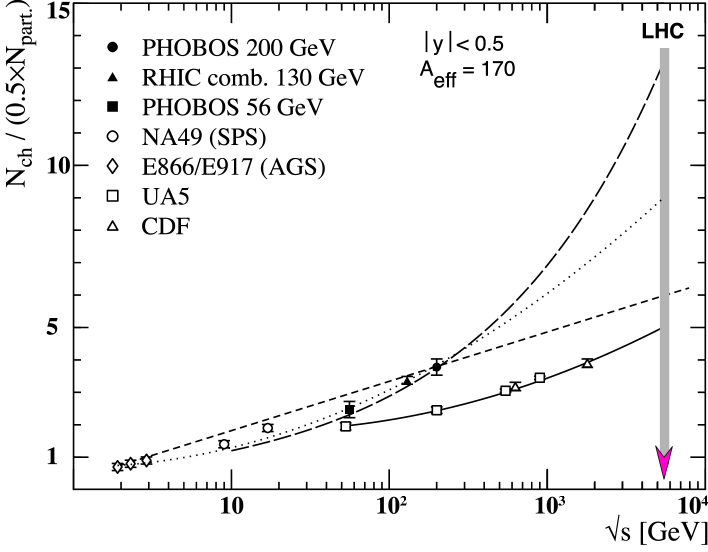
In fig. 1 the charged multiplicity normalized to the number of participant pairs as a function of the centre-of-mass energy is shown for Au–Au data at RHIC (closed symbols) and a variety of pp data (open symbols). Assuming universality, a fit for the extrapolation to the LHC energy of all nuclear data to eq. (2), gives $b=0.68$ and $c=0.26$ for $a=0$ fixed (dashed line), and $a=0.028$ and $c=0.7$ for $b=0$ fixed (dotted line). The long-dashed line is the extrapolation given by the saturation model (EKRT) [14]. Like most models in that context (see LABEL:kharzeev2000 and references therein) it assumes that the phase space available for quarks and gluons saturates at some dynamical energy scale $Q_{\rm sat,A}(\sqrt{s})$, the saturation scale, at which, by the uncertainty, principle the parton wave functions start to overlap in the transverse plane.  In such a scenario the total multiplicity basically is determined by the transverse energy density per unit rapidity.

$$N(\sqrt{s})\sim Q^{2}_{\rm sat,A}(\sqrt{s})\,R^{2}_{\rm A}\sim A^{\alpha}\,\sqrt{s}^{\beta}\;,$$ (3)

The original EKRT result [14] —refined in LABEL:eskola2001— for $\alpha=0.922$, $\beta=0.383$ and a proportionality constant of $1.383$ quite successfully predicted the RHIC multiplicities. A very recent estimation [17], using the argument of geometrical scaling found at small-x lepton-proton data from HERA extended to nuclear photo-absorption cross sections, finds eq. (3) with $\alpha=0.089$, $\beta=0.288$ and a proportionality constant of $0.5$.

For the extrapolation to LHC energies, the crucial point is, whether the total multiplicity as a function of $\sqrt{s}$ has a power-law behaviour like eq. (3) or rather grows with the power of the logarithm like eq. (2). The range within RHIC is small and that from RHIC to LHC is large (see fig. 1). There is a lot of room for error, as within RHIC one cannot reliably distinguish between the different parametrical descriptions.

Model	$N_{\rm ch}$	Comments
$\ln s$ fit	$\simeq$ 1000	eq. (2); $a=0$, $b=0.68$, $c=0.26$
$\ln^{2}s$ fit	$\simeq$ 1500	eq. (2); $a=0.028$, $b=0$, $c=0.7$
EKRT	$\simeq$ 2200	eq. (3); $\alpha=0.922$, $\beta=0.383$, $\mathrm{const}=1.383$
Geom. scaling	$\simeq$ 1700	eq. (3); $\alpha=0.089$, $\beta=0.288$, $\mathrm{const}=0.5$
Initial parton saturation	$\simeq$ 1900	eq. (3), but calculated from CGC [18]
HIJING 1.36	$\simeq$ 6200	with quenching
	$\simeq$ 2900	without quenching
DPMJET-II.5	$\simeq$ 2300	with baryon stopping
	$\simeq$ 2000	without baryon stopping
SFM	$\simeq$ 2700	with fusion
	$\simeq$ 3100	without fusion

Table 1: Charged-particle multiplicity predictions of different models at $\eta\approx 0$.

In table 1 we summarize the expectations of the charged-particle multiplicity at mid-pseudo-rapidity for the different models. 

In addition to estimates already mentioned, we quote the predictions for various Monte Carlo event generators. At the time of the ALICE technical proposal [19] and before the start-up of RHIC, the predictions for Pb–Pb collisions at $\sqrt{s_{\scriptscriptstyle{{\rm NN}}}}=5.5\leavevmode\nobreak\ \mbox{${\rm TeV}$}$ ranged between $1500$–$8000$ charged particles at central rapidity [20]. Now most generators have been updated, of which we mention HIJING, DPMJET and SFM. HIJING is a QCD-inspired model of jet production [21, 22] with the Lund model [23] for jet fragmentation. The multiplicity in central events with and without jet quenching differs by more than a factor of 2. Including jet quenching it predicts the highest multiplicities of all models. The DPMJET model [24] is an implementation of the two-component Dual Parton Model (DPM) [25] based on the Glauber–Gribov approach. It treats soft and hard scattering processes in an unified way and uses the Lund model [23] for fragmentation. Predictions with and without the baryon stopping mechanism are shown, and baryon stopping increases the multiplicity by about 15%. The String Fusion Model (SFM) [26] includes in its initial stage both soft and semi-hard components leading to the formation of colour strings. Collectivity is taken into account by means of string fusion and string breaking leads to the production of secondaries. Predictions with string fusion reduce the multiplicity by about 10% compared to calculations without fusion.

The large variety of available models of heavy-ion collisions gives a wide range of predicted multiplicities from $1000$ to $6200$ charged particles at mid-rapidity for central Pb–Pb collisions. The multiplicity measured at RHIC, $\mathrm{d}N_{\mathrm{ch}}/\mathrm{d}\eta\simeq 750$ ($\mathrm{d}N_{\mathrm{ch}}/\mathrm{d}y\simeq 650$), at $\sqrt{s_{\scriptscriptstyle{{\rm NN}}}}=200\leavevmode\nobreak\ \mbox{${\rm GeV}$}$, was found to be about a factor 2 lower than what was predicted by most models [27]. In view of this fact, the multiplicity at the LHC is probably between $1500$ and $3000$ charged particles per unit of rapidity. Though, as we will briefly touch on in chapter 3 the ALICE detectors are designed to cope with multiplicities up to 8000 charged particles per rapidity unit, a value which ensures a comfortable safety margin.

3 Deconfinement region

Starting from the estimates of the charged multiplicity or average transverse energy, most parameters of the medium produced in the collision can be inferred by assuming (local) thermodynamical equilibrium with a certain equation of state. Because of its simplicity, one often considers the energy density of an equilibrated ideal gas of particles with $n_{\rm dof}$ degrees of freedom [28]

$$\varepsilon=n_{\rm dof}\,\frac{\pi^{2}}{30}\,T^{4}$$ (4)

according to the Stefan-Boltzmann law. For a pion gas the degrees of freedom are only the three values of the iso-spin for $\pi^{+},\,\pi^{0},\,\pi^{-}$. For a QGP with two quark flavours the degrees of freedom are $n_{g}+7/8\,(n_{q}+n_{\bar{q}})=N_{g}(8)\,N_{\rm pol}(2)+7/8\,\times 2\times N_{\rm flav}(2)\,N_{\rm col}(3)\,N_{\rm spin}(2)=37$. The factor 7/8 accounts for the difference between Bose-Einstein for gluons and Fermi-Dirac statistics for quarks.

Parameter		SPS	RHIC	LHC
$\sqrt{s_{\scriptscriptstyle{{\rm NN}}}}$	[${\rm GeV}$]	$17$	$200$	$5500$
d$N_{\rm gluons}/$d$y$		$450$	$1200$	$4700$
$\mathrm{d}N_{\mathrm{ch}}/\mathrm{d}y$		$350$	$800$	$3000$
$Q_{\rm sat,A}$	[${\rm GeV}$]	$0.71$	$1.13$	$2.13$
Initial temperature	[${\rm GeV}$]	$0.38$	$0.6$	$>1$
Initial energy density	[$\mbox{${\rm GeV}$}/\mbox{${\rm fm}$}^{3}$]	$\sim 5$	$\sim 25$	$\sim 250$
Freeze-out volume	[$\mbox{${\rm fm}$}^{3}$]	$\sim 10^{3}$	$\sim 10^{4}$	$\sim 10^{5}$
Life time	[${\rm fm}$]	$<2$	$2$-$4$	$>10$

Table 2: Comparison of the most relevant—model-dependent—parameters characterizing central nucleus–nucleus collisions at different energy scales [14].

In table 2 we present a comparison of the most relevant —model-dependent—parameters for SPS, RHIC and LHC energies, where the equation of state describes a free gas of gluons [$n_{\rm dof}=16$ in eq. (4)] and adiabatic longitudinal expansion is included in the hydrodynamical calculation [14]. A slightly refined calculation [16] using an equation of state with quark and gluonic degrees of freedom and including transverse expansion in the hydrodynamical phase as well as hadronic resonances (and decays) at freeze-out (see LABEL:sollfrank1996) gives only slightly different results of the order of $10$–$15$%.

The high energy in the collision centre-of-mass at the LHC determines a very large energy density and an initial temperature at least a factor 2 higher than at RHIC. The high initial temperature extends the life time and the volume of the deconfined medium, since the QGP has to expand while cooling down to the critical (or freeze-out) temperature, which is about $175\pm 15\leavevmode\nobreak\ \mbox{${\rm MeV}$}$ and relatively independent of $\sqrt{s}$ above the SPS energy (see fig. 2). In addition, the large number of gluons favours energy and momentum exchanges, thus considerably reducing the time needed for the thermal equilibration of the medium. Thus, the LHC will create a hotter, larger and longer-living QGP state than the present heavy-ion facilities. The main advantage is due to the fact that in the deconfinement scenario the QGP is more similar to the thermodynamical equilibrated QGP theoretically investigated by means of (Euclidian) lattice QCD [30, 31, 32, 33, 34, 35] and of statistical hadronization models [36, 37]. Both methods—and further phenomenological models (see LABEL:stephanov2004 and references therein)— map out the different phase boundaries of strongly interacting matter described by QCD.

1 Phase diagram of strongly interacting matter

The current knowledge of the phase diagram [39] is displayed in fig. 2 as a function of the temperature, $T$, and of the baryo-chemical potential, $\mu_{\rm B}$, as a measure of the baryonic density. 

At low temperatures and for $\mu_{\rm B}\simeq m_{\rm p}\simeq 1\leavevmode\nobreak\ \mbox{${\rm GeV}$}$, there is the region of the ordinary matter of protons and neutrons. Increasing the energy density of the system, by ‘compression’ (towards the right) or by ‘heating’ (upward), the hadronic gas phase is reached in which nucleons interact and form pions, excited states of the proton and of the neutron such as $\Delta$ resonances and other hadrons. If the energy density is further increased, the transition to the deconfined QGP phase is predicted [40]: the density of the partons, quarks and gluons, becomes high enough that the confinement of quarks in hadrons vanishes (deconfinement).

The phase transition can be reached along different ‘paths’ on the ($\mu_{\rm B}$, $T$) plane. In heavy-ion collisions, both, temperature and density increase, possibly bringing the system beyond the phase boundary. In fig. 2 the regions of the fixed-target (AGS, SPS) and collider (RHIC) experiments are shown, as well as the freeze-out temperatures and densities from $\chi^{2}$-minimization fits of the measured particle yields versus the yields calculated from the statistical partition function of an ideal hadron-resonance gas for two different approaches: the Statistical Hadronization Model (SHM) [36] and the Thermal Hadronization Model (THM) [37]). THM assumes full thermodynamical equilibrium using the grand canonical ensemble, whereas SHM allows the non-equilibrium fluctuation of the total strangeness content by introducing one additional parameter ($\gamma_{\rm S}$) to account for the suppression of hadrons containing valence strange-quarks.

A more fundamental, complementary method to explore the qualitative features of the QGP and to quantify its properties is the numerical evaluation of expectation values from path-integrals in discrete space-time on a lattice [41].  As phase transitions are related to large-distance phenomena, implying correlations over a large volume, and because of the increasing strength of QCD interactions with distance, such phenomena cannot be treated using perturbative methods.

Figure 2: The phase diagram of strongly interacting QCD matter as a function of the temperature $T$ and of the baryonic chemical potential $\mu_{\rm B}$. The freeze-out points for SHM are taken from LABEL:becattini2004 and for THM from LABEL:braun-munzinger2003; the lattice point in the chiral limit at $\mu_{\rm B}=0$ for two flavours from LABEL:karsch2000 and the phase-boundary curves for $2+1$ flavours (red curve) with physical quark masses from LABEL:fodor2004 and three flavours (blue curve) from LABEL:karsch2003b in the chiral limit. When available, statistical errors are shown.

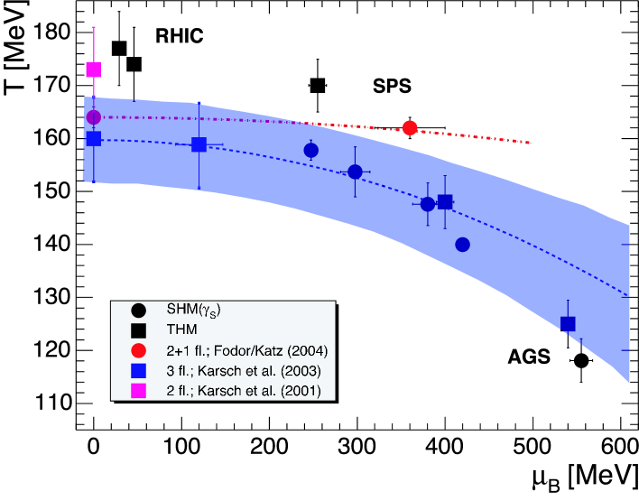
Lattice calculations are most reliably performed for a baryon-free system, as the introduction of a finite potential $\mu_{\rm B}\neq 0$ in the Wick-rotated Euclidian path-integrals imposes severe problems for the numerical Monte Carlo evaluation.  Recently, several methods have been introduced allowing one to address moderate chemical potentials on the lattice [44]. The results obtained from different lattice calculations are shown in fig. 2 for a $2$-flavours calculation in the chiral limit [32] and two very recent calculations of the phase boundary: $2+1$ flavours with physical quark masses [31] and three flavours in the chiral limit [34]. The precise location of the various phase points and the nature of the phase transition vary quantitatively but also qualitatively depending on the number of flavours, their (bare) masses and the extrapolation to the chiral and continuum limit (if done at all). These recent results support the following picture: The phase transition is of first order starting from ($T$, $\mu_{\rm B}$) at low temperature and high density till the critical end-point ($T_{\rm C}^{\rm E}$, $\mu_{\rm B}^{\rm E}$) at low baryo-chemical potentials of about $100$–$500\leavevmode\nobreak\ \mbox{${\rm MeV}$}$ followed by a cross-over region until ($T_{\rm C}$, $0$).  The exact location of the end-point is of great interest for the heavy-ion community. Its precise determination, however, highly depends on the values for the quark masses used on the lattice.

2 Towards the Stefan-Boltzmann limit

The cross-over, however, is expected to take place in a narrow temperature interval, which makes the transition between the hadronic and partonic phases quite well localized. This is reflected in a rapid rise of the energy density in the vicinity of the cross-over temperature in fig. 3 for lattice calculations at $\mu_{\rm B}=0$. Shown is the normalized energy density $\varepsilon/T^{4}$ as a function of $T$ for the pure gauge sector of QCD alone, for $2$- and $3$-flavours QCD in the chiral limit, as well as the expected form for the case of two degenerate light and one heavier (strange) quark with $m_{\rm s}\sim T_{\rm C}$ (indicated by the stars) [45].

The number of flavours and the masses of the quarks constitute the main uncertainties in the determination of the critical temperature and critical energy density. They are estimated to be $T_{\rm C}=175\pm 15\leavevmode\nobreak\ \mbox{${\rm MeV}$}$ and $\varepsilon_{\rm C}/T_{\rm C}^{4}\simeq 6\pm 2$ leading to $\varepsilon_{\rm C}\simeq 0.3$–$1.3\leavevmode\nobreak\ \mbox{${\rm GeV}$}/\mbox{${\rm fm}$}^{3}$. Clearly, the transition is not of first order, which would be characterized by a discontinuity of $\varepsilon$ at $T=T_{\rm C}$. However, a large increase of $\Delta\varepsilon/T_{\rm C}^{4}\simeq 8$ in the energy density is observed in a small temperature interval of only about $20$–$40\leavevmode\nobreak\ \mbox{${\rm MeV}$}$ for the $2$-flavours calculation.  The dramatic increase of $\varepsilon/T^{4}$ is related to the change of $n_{\rm dof}$ in eq. (4) from 3 in the pion-gas phase to $37$ for two flavours and $47.5$ for three flavours in the deconfined phase, as soon as the additional colour and quark flavour degrees of freedom become available. The transition temperature for the physically realized quark-mass spectrum ($2+1$-flavours QCD) is expected to be close to the value for two flavours, since the strange quarks have a mass of $m_{\rm s}\sim T_{\rm C}$ and therefore do not contribute to the physics at a temperature close to $T_{\rm C}$, but will do so at higher temperature.

In general, $\mu_{\rm B}=0$ is not valid for heavy-ion collisions, since the two colliding nuclei carry a total baryon number equal to twice their mass number. But, the baryon content of the system after the collision is expected to be concentrated rather near the rapidity of the two colliding nuclei. Therefore, the larger the rapidity of the beams, with respect to their centre of mass, the lower the baryo-chemical potential in the central rapidity region. The rapidities of the beams at SPS, RHIC and LHC are 2.9, 5.3 and 8.6, respectively. Thus, the LHC at mid-rapidity is expected to be much more baryon-free than RHIC and closer to the conditions simulated in lattice QCD for $\mu_{\rm B}=0$.

Figure 3: The (normalized) energy density in QCD with different (degenerate) quark flavours at $\mu_{\rm B}=0$ in the chiral limit and a sketch of the expected form of the energy density for QCD with two degenerate light quarks and a fixed strange quark mass $m_{\rm s}\sim T_{\rm C}$ [45]. The arrows indicating the energy densities reached in the initial stage of heavy-ion collisions at the SPS, RHIC and LHC are based on the Bjorken estimate, eq. (1). The arrows on the right-side ordinates show the value of the Stefan-Boltzmann limit for an ideal quark-gluon gas, eq. (4).

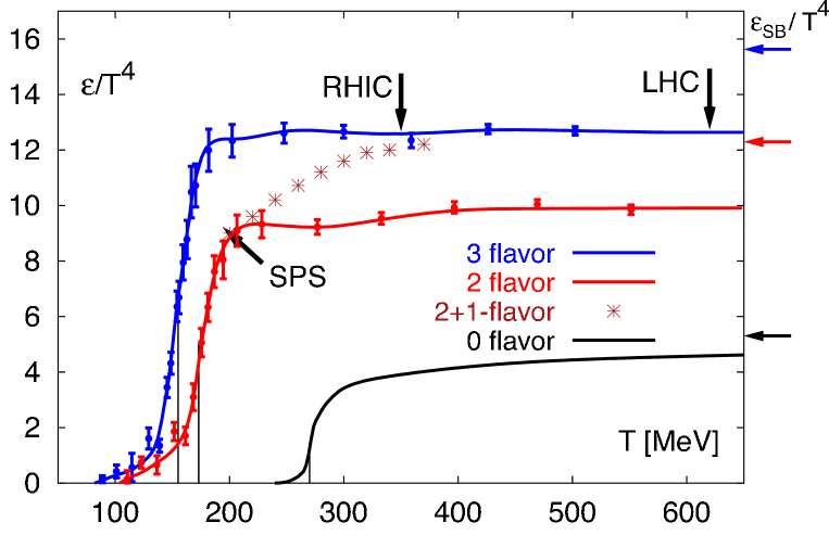
The difference of $\varepsilon$ computed on the lattice compared to the Stefan-Boltzmann limit calculated from eq. (4) with $n_{\rm dof}=16$ (gluons only), $37$ (two flavours) and $47.5$ (three flavours) (see fig. 3) indicates that significant non-perturbative effects are to be expected at least up to temperatures $T\simeq(2$-$3)\,T_{\rm C}$. The strong coupling constant in the range $T\geq T_{\rm C}$ is estimated [46] as

$$\alpha_{\rm S}(T)=\frac{4\pi}{18\,\ln(5\,T/\Lambda_{\rm QCD})}=\left\{\begin{array}[]{ll}0.43&{\rm for}\leavevmode\nobreak\ T=T_{\rm C}\\ 0.3&{\rm for}\leavevmode\nobreak\ T=2\,T_{\rm C}\\ 0.23&{\rm for}\leavevmode\nobreak\ T=4\,T_{\rm C}\\ \end{array}\right.$$

where the numbers are obtained by using the fact that the QCD scaling constant $\Lambda_{\rm QCD}\approx 200\leavevmode\nobreak\ \mbox{${\rm MeV}$}$ is of the same order of magnitude as $T_{\rm C}$. The values for $\alpha_{\rm S}$ confirm that non-perturbative effects are still sizeable in the range $T<2\,T_{\rm C}$, where the QCD recently has been called sQGP [47]. With an initial temperature of about $4$–$6\leavevmode\nobreak\ T_{\rm C}$ predicted for central Pb–Pb collisions at $\sqrt{s_{\scriptscriptstyle{{\rm NN}}}}=5.5\leavevmode\nobreak\ \mbox{${\rm TeV}$}$ (see table 2), the LHC will provide quite ideal conditions (with smaller non-perturbative effects) possibly allowing a direct comparison to perturbative calculations:

4 Novel kinematical range

Heavy-ion collisions at the LHC access not only a quantitatively different regime of much higher energy density providing ideal initial conditions, but also a qualitatively new regime of parton kinematics, mainly because:

• Saturated parton distributions dominate particle production;

• Hard processes contribute significantly to the total A–A cross section.

1 Low-x parton distribution functions

In the inelastic, hard collision of an elementary particle with an hadron, the Bjorken-$x$ variable (in the infinite-momentum frame) is essentially determined by the fraction of the hadron momentum carried by the parton that enters the hard scattering process. The hard scatter is characterized by the momentum transfer squared, $Q^{2}=-q^{2}$, between the elementary particle and the participating parton in the inelastic scattering process. $Q$ is called the virtuality and typically represents the hard-scattering scale of pQCD [48].

(a) Structure function, $F_{2}$

(b) Comparison of global fits

Figure 4: 4(a) $F_{2}$ (from pure $\gamma$ exchange) from HERA and fixed target experiments compared with ZEUS NLO QCD fit. 4(b) Comparison of the Parton Distribution Functions from the ZEUS fit [49] to global fits by MRST2001 [50] and CTEQ 6M [51]. Both figures are taken from LABEL:werner2003.

The momentum-fraction distribution for a given parton type (e.g. gluon, valence quark, sea quark), $f_{i}(x)$, is called PDF. It gives the probability that a parton of type $i$ carries a fraction $x$ of the hadron’s (longitudinal) momentum. The PDF cannot be computed by perturbative methods and, so far, it has not been possible to compute them with lattice methods either. Thus, non-perturbative input from data on various hard processes must be taken for its extraction. The momentum distributions of partons within a hadron are assumed to be universal, which is one of the essential features of QCD. In other words, the PDFs derived from any process can be applied to other processes. Uncertainties from the PDFs result from uncertainty in the input data. The main experimental knowledge on the proton PDFs comes from Deep Inelastic Scattering (DIS) measuring the proton structure functions, in particular from HERA for the small-$x$ region [52, 49].

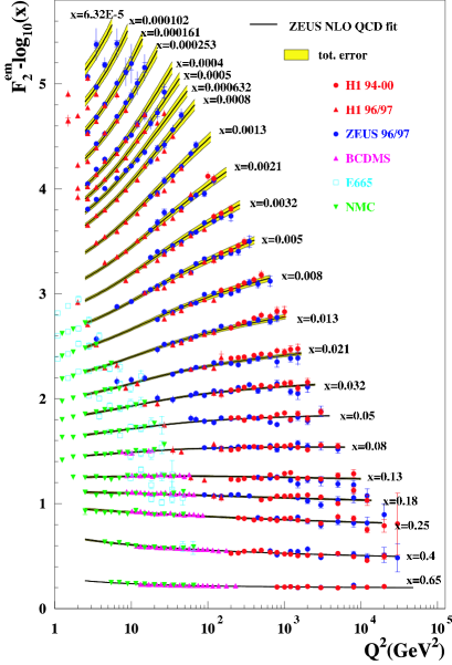
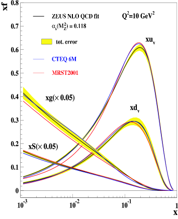
Figure 4(a) shows the proton structure function $F_{2}(x,Q^{2})$ measured at H1 and ZEUS together with data from fixed-target experiments. The steep rise of $F_{2}$ at small $x$ is driven by the gluons. The data are spread over four orders of magnitude in $x$ and $Q^{2}$ and are well described by the Dokshitzer-Gribov-Lipatov-Altarelli-Parisi (DGLAP) parton evolution [53, 54, 55, 56].

Several groups (MRST [57, 50], CTEQ [58, 59, 51], GRV [60]) have developed parametrizations for the PDFs by global fits to most of the available DIS data, where typically the PDFs are parametrized at a fixed starting scale $Q^{2}=Q^{2}_{0}$ and determined by a Next-to-Leading Order (NLO) QCD fitting procedure.  Using the framework of DGLAP for parton evolution in pQCD one then can extrapolate the PDFs at different kinematical ranges. The extracted PDFs derived by ZEUS [49] at the scale of $Q^{2}=10\leavevmode\nobreak\ \mbox{${\rm GeV}$}^{2}$ compared to the global analyses of MRST2001 [50] and CTEQ 6M [51] are shown in fig. 4(b). Within the estimated total error on the PDFs the different sets are consistent.

(a) $Q=10\leavevmode\nobreak\ \mbox{${\rm GeV}$}$

(b) $Q=100\leavevmode\nobreak\ \mbox{${\rm GeV}$}$

Figure 5: The CTEQ 4L parametrization of the proton PDFs for valence quarks, sea quarks and gluons inside the proton at the scale of $Q=10\leavevmode\nobreak\ \mbox{${\rm GeV}$}$ and $Q=100\leavevmode\nobreak\ \mbox{${\rm GeV}$}$.

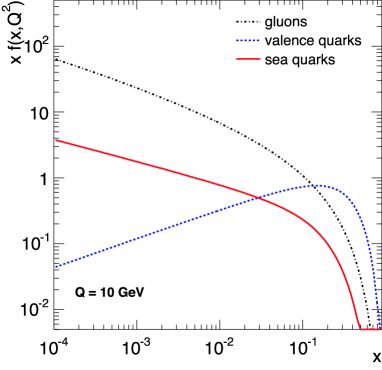
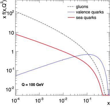
Figure 5 shows the PDFs of valence quarks, sea quarks and gluons inside the proton at two scales, $Q=10\leavevmode\nobreak\ \mbox{${\rm GeV}$}$ and $Q=100\leavevmode\nobreak\ \mbox{${\rm GeV}$}$, in the CTEQ 4L parametrization [58]. Note that the PDFs are weighted by $x$ to indicate the differences between the parton types, which somewhat hides the strong growth of the gluon and sea quark contribution at small $x$. We shall see in the next section that at LHC values of $x\,{\buildrel>\over{{}_{\sim}}}\,0.005$ contribute to the production of jets at mid-rapidity.

2 Accessible x-range at the LHC

At the LHC the PDFs of the nucleon and, in the case of p–A and A–A collisions, their modifications in the nucleus, will be probed down to unprecedented low values of $x$. In the following, we consider the case of the production of a dijet through LO two-parton kinematics $p_{1}+p_{2}=p_{3}+p_{4}$ (e.g. gluon–gluon, quark–qluon or quark–quark scattering) in the collision of two ions ($A_{1}$, $Z_{1}$) and ($A_{2}$, $Z_{2}$).  The $x$ range actually probed depends on the value of the centre-of-mass energy per nucleon pair $\sqrt{s_{\scriptscriptstyle{{\rm NN}}}}$, on the invariant mass $M_{\rm jj}$ of the dijet produced in the hard scattering representing the virtuality of the process and on its rapidity $y_{\rm jj}$. Neglecting the intrinsic transverse momenta of the partons in the nucleon, we can approximate the four-momenta of the two incoming partons by $p_{1}=(x_{1},0,0,x_{1})\,Z_{1}/A_{1}\,\sqrt{s_{\rm pp}}/2$ and $p_{2}=(x_{2},0,0,-x_{2})\,Z_{2}/A_{2}\,\sqrt{s_{\rm pp}}/2$, where $x_{1}$ and $x_{2}$ are the momentum fractions carried by the partons, and $\sqrt{s_{\rm pp}}$ is the centre-of-mass energy for pp collisions ($14\leavevmode\nobreak\ \mbox{${\rm TeV}$}$ at the LHC). Thus, we derive the square of the invariant mass of the dijet

$$M^{2}_{\rm jj}=\hat{s}=x_{1}\,x_{2}\,s_{\rm NN}=x_{1}\,\frac{Z_{1}}{A_{1}}\,x_{2}\,\frac{Z_{2}}{A_{2}}\,s_{\rm pp}$$

and its longitudinal rapidity in the laboratory system

$$y_{\rm jj}=\frac{1}{2}\ln\left[\frac{E+p_{z}}{E-p_{z}}\right]=\frac{1}{2}\ln\left[\frac{x_{1}}{x_{2}}\,\frac{Z_{1}\,A_{2}}{Z_{2}\,A_{1}}\right]\;.$$

From the two relations we get the dependence of $x_{1}$ and $x_{2}$ on the properties of the colliding system, $M_{\rm jj}$ and $y_{\rm jj}$, as

$$x_{1}=\frac{A_{1}}{Z_{1}}\,\frac{M_{\rm jj}}{\sqrt{s_{\rm pp}}}\exp\left({+y_{\rm jj}}\right)\hskip 14.22636pt\text{and}\hskip 14.22636ptx_{2}=\frac{A_{2}}{Z_{2}}\,\frac{M_{\rm jj}}{\sqrt{s_{\rm pp}}}\exp\left({-y_{\rm jj}}\right)\;,$$

which for a symmetric colliding system ($A_{1}=A_{2}$, $Z_{1}=Z_{2}$) simplifies to

$$x_{1}=\frac{M_{\rm jj}}{\sqrt{s_{\scriptscriptstyle{{\rm NN}}}}}\exp\left({+y_{\rm jj}}\right)\hskip 14.22636pt\text{and}\hskip 14.22636ptx_{2}=\frac{M_{\rm jj}}{\sqrt{s_{\scriptscriptstyle{{\rm NN}}}}}\exp\left({-y_{\rm jj}}\right)\;.$$

In the case of asymmetric collisions, as p–Pb and Pb–p, the centre of mass moves with a longitudinal rapidity

$$y_{\rm c.m.}=\frac{1}{2}\ln\left(\frac{\rm Z_{1}A_{2}}{\rm Z_{2}A_{1}}\right)$$

and the rapidity window covered by the experiment is consequently shifted by

$$\Delta y=y_{\rm lab.\leavevmode\nobreak\ system}-y_{\rm c.m.\leavevmode\nobreak\ system}=y_{\rm c.m.}$$

corresponding to $+0.47$ ($-0.47$) for p–Pb (Pb–p) collisions. Therefore, running with both p–Pb and Pb–p will allow one to cover the largest interval in Bjorken-$x$.

Figure 6: The range of Bjorken-$x$ and $M^{2}$ relevant for particle production in A–A collisions at the top SPS, RHIC and LHC energies. Lines of constant rapidity are indicated.

Machine	SPS	RHIC	LHC	LHC
System	Pb–Pb	Au–Au	Pb–Pb	pp
$\sqrt{s_{\scriptscriptstyle{{\rm NN}}}}$	17 ${\rm GeV}$	200 ${\rm GeV}$	5.5 ${\rm TeV}$	14 ${\rm TeV}$
$E_{\mathrm{T}}=10\color[rgb]{1,1,1}0\color[rgb]{0,0,0}\leavevmode\nobreak\ \mbox{${\rm GeV}$}$	$x\simeq 1.18$	$x\simeq 0.10$	$x\simeq 0.004$	$x\simeq 0.001$
$E_{\mathrm{T}}=25\color[rgb]{1,1,1}0\color[rgb]{0,0,0}\leavevmode\nobreak\ \mbox{${\rm GeV}$}$	-	$x\simeq 0.25$	$x\simeq 0.009$	$x\simeq 0.004$
$E_{\mathrm{T}}=50\color[rgb]{1,1,1}0\color[rgb]{0,0,0}\leavevmode\nobreak\ \mbox{${\rm GeV}$}$	-	$x\simeq 0.50$	$x\simeq 0.018$	$x\simeq 0.007$
$E_{\mathrm{T}}=100\leavevmode\nobreak\ \mbox{${\rm GeV}$}$	-	-	$x\simeq 0.036$	$x\simeq 0.014$
$E_{\mathrm{T}}=200\leavevmode\nobreak\ \mbox{${\rm GeV}$}$	-	-	$x\simeq 0.072$	$x\simeq 0.028$

Table 3: Bjorken-$x$ values probed by jet production at various transverse jet energies for different systems at mid-rapidity.

Figure 6 shows the range of accessible values of Bjorken-$x$ in nucleus–nucleus collisions at the SPS, RHIC and LHC energies. Clearly, the LHC will open a novel regime of $x$-values as low as $10^{-5}$, where strong gluon shadowing is expected and the initial gluon density is close to saturation, such that the time evolution of the system might be described by classical chromodynamics (see section 3).

At central rapidities for $y_{\rm jj}\approx 0$ we have $x_{1}\simeq x_{2}$, and their magnitude is determined by the ratio of the invariant mass to the centre-of-mass energy. The invariant dijet mass is given by the transverse jet energy, $M_{\rm jj}=2\,E_{\mathrm{T}}\simeq 2\,p_{\mathrm{T}}$; therefore with $x_{\mathrm{T}}=2\,p_{\mathrm{T}}/\sqrt{s_{\scriptscriptstyle{{\rm NN}}}}$ we get $x_{1}\simeq x_{2}\simeq x_{\mathrm{T}}$. In terms of the outgoing parton momenta, $p_{1}+p_{2}=p_{3}+p_{4}$, we find by applying momentum conservation (at LO)

$$x_{1}=\frac{1}{2}\,x_{\mathrm{T}}\,\left(e^{y_{3}}+e^{y_{4}}\right)\hskip 14.22636pt\text{and}\hskip 14.22636ptx_{2}=\frac{1}{2}\,x_{\mathrm{T}}\,\left(e^{-y_{3}}+e^{-y_{4}}\right)\;.$$ (5)

Table 3 reports the Bjorken-$x$ values for jets with transverse energy between $E_{\mathrm{T}}=10\leavevmode\nobreak\ \mbox{${\rm GeV}$}$ and $E_{\mathrm{T}}=200\leavevmode\nobreak\ \mbox{${\rm GeV}$}$ for a variety of systems. The $x$-regime relevant for jet production of $50$–$200$ ${\rm GeV}$ at LHC ($0.005\,{\buildrel<\over{{}_{\sim}}}\,x\,{\buildrel<\over{{}_{\sim}}}\,0.1$) is between one and two orders of magnitude smaller than at RHIC, where the cross section for the hard jets ($E_{\mathrm{T}}\geq 50\leavevmode\nobreak\ \mbox{${\rm GeV}$}$) is essentially zero (see table 4).

3 Nuclear-modified parton distribution functions

So far, we have looked at the PDFs extracted from the structure function $F_{2}$ of the free proton. Experimentally for various nuclei, the ratios of $F_{2}^{A}$ to the structure function of deuterium, $F_{2}^{A}(x,Q^{2})/F_{2}^{D}(x,Q^{2})$, reveal clear deviations from unity. This indicates that the parton distributions of bound protons are different from those of the free protons, $f_{i/\rm A}(x,Q^{2})\neq f_{i}(x,Q^{2})$. The nuclear effects in the ratio $F_{2}^{A}/F_{2}^{D}$ are usually divided into the following regions in Bjorken $x$:

• Fermi motion, an excess for $x\rightarrow 1$ and beyond;

• EMC effect, a depletion at $0.3\,{\buildrel<\over{{}_{\sim}}}\,x\,{\buildrel<\over{{}_{\sim}}}\,0.7$;

• anti-shadowing, an excess at $0.1\,{\buildrel<\over{{}_{\sim}}}\,x\,{\buildrel<\over{{}_{\sim}}}\,0.3$;

• nuclear shadowing, a depletion at $x\,{\buildrel<\over{{}_{\sim}}}\,0.1$;

• saturation effect, saturation of the depletion at $x\,{\buildrel<\over{{}_{\sim}}}\,0.001$.

Figure 7: Ratio of the gluon distribution in the lead nucleus over the gluon distribution in the proton for different models at $Q^{2}=5\leavevmode\nobreak\ \mbox{${\rm GeV}$}^{2}$, corresponding to $\mathrm{c\overline{c}}$ production at threshold. The $x$-region for the production at RHIC and LHC are highlighted. The figure is taken from LABEL:armesto2003, which lists the original references to the model calculations.

Currently, there is no unique theoretical description of these effects. It is believed that different mechanisms are responsible for them in different kinematic regions [64]. In a very simplified picture, the extension of the Bjorken-$x$ range down to about $10^{-3}$–$10^{-5}$ at the LHC means that a large-$x$ parton in one of the two colliding lead nuclei resolves the other incoming nucleus as a superposition of about ${\rm A}\times 10^{3}$–$10^{5}$ $\approx 10^{5}$–$10^{7}$ gluons. Thus, there are many incoming small-$x$ gluons, which are densely packed and have a large wave-length (via the Heisenberg uncertainty) so that the low-momentum gluons tend to merge together: two gluons with momentum fractions $x_{1}$ and $x_{2}$ combine into a single gluon with momentum fraction $x_{1}+x_{2}$ ($g_{x_{1}}g_{x_{2}}\to g_{x_{1}+x_{2}}$). As a consequence of the combination process towards larger $x$, affecting not only gluons, but all partons, the nuclear parton densities are depleted in the small-$x$ region ($x\,{\buildrel<\over{{}_{\sim}}}\,0.1$) and slightly enhanced in the large-$x$ region ($0.1\,{\buildrel<\over{{}_{\sim}}}\,x\,{\buildrel<\over{{}_{\sim}}}\,0.3$) with respect to the parton densities of the proton. Eventually at certain small-$x$ values, the nuclear gluon densities saturate as a result of non-linear corrections to the DGLAP evolution equations [65, 66, 67]. The saturation scale, which is proportional to the gluon density per unit area and grows as $Q^{2}_{\rm sat,A}\sim A^{1/3}/x^{\delta}$ ($\delta\approx 0.2$–$0.3$ at HERA), determines the critical values of the momentum transfer, at which the parton systems becomes dense and recombination frequently happens. At LHC the expected saturation scale, $Q_{\rm sat,A}>2\leavevmode\nobreak\ \mbox{${\rm GeV}$}$, is in the perturbative regime and heavy-ion collisions are depicted as a collision of dense gluon walls. 

Figure 8: Ratio of the gluon distribution in the lead nucleus over the gluon distribution in the proton for EKS98 parametrization for different scales.

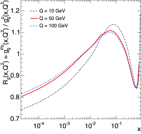
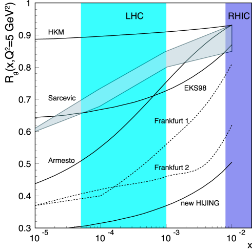
Recently, the nuclear shadowing effect has been analysed in the DGLAP framework using data from electron–nucleus DIS in the range $0.005<x<1$ [69]. However, no data are available in the complete $x$-range covered by the LHC and the existing data provide only weak constraints for the gluon PDFs, which enter the measured structure functions at NLO. Two groups, EKRS [70, 71] and HKM [72], applied the same strategies as in the case of the proton PDFs, in order to obtain a parametrization (and extrapolation to low-$x$ values) of the nuclear-modified Parton Distribution Functions.  There are a couple of other models, which try to describe nPDFs. Though they all tend to disagree, where no experimental constraints are available. The present situation is summarized [63] in fig. 7 representing the results of the different models as the ratio of the gluon distribution in the lead nucleus over the gluon distribution in the proton,

$$R_{g}(x,Q^{2})=\frac{g^{\rm Pb}(x,Q^{2})}{g^{\rm p}(x,Q^{2})}\;.$$ (6)

The predictions for the gluon shadowing, $g(x\sim 10^{-3}$–$10^{-5})$, at the LHC range between 30% and 90%. The large uncertainty might be reduced in the future by more data from nuclear DIS, p–A data collected at RHIC and by the measurements of charm and beauty production in p–Pb at the LHC [61].

In fig. 8 we show the ratio eq. (6) for the EKS98 parametrization [71] as a function of $x$ for different scales. The deviation from the proton PDF in relevant region for jet production at mid-pseudo-rapidity ($0.005\,{\buildrel<\over{{}_{\sim}}}\,x\,{\buildrel<\over{{}_{\sim}}}\,0.1$) is about 10%. Therefore, if not otherwise indicated, we often neglect the nuclear modification of the PDFs in the present work.

4 Hard scattering processes

Hard processes are expected to be abundant at LHC energies. Practically in every minimum-bias event at the LHC high-$p_{\mathrm{T}}$ partons are expected to be produced in scattering processes at $Q^{2}\gg\Lambda^{2}_{\rm QCD}$.  At the scale much larger than $\Lambda_{\rm QCD}\simeq 200\leavevmode\nobreak\ \mbox{${\rm MeV}$}$, these hard processes can be calculated using pQCD and are expected to be under reasonable theoretical control. Since high-$p_{\mathrm{T}}$ partons tend to fragment hard, the measured transverse-momentum spectrum is expected to be harder than at RHIC or SPS.

Figure 9: The predicted, LO, differential cross section for neutral pion and inclusive charged hadron production in pp collisions at mid-rapidity ($y=0$) for $\sqrt{s_{\scriptscriptstyle{{\rm NN}}}}=17,\leavevmode\nobreak\ 200,\leavevmode\nobreak\ 5500\leavevmode\nobreak\ \mbox{${\rm GeV}$}$. The figure is taken from LABEL:vitev2002. (All scales are set to $p_{\mathrm{T}}^{2}$ and $\left<{k}_{\rm T}^{2}\right>=1.8\leavevmode\nobreak\ \mbox{${\rm GeV}$}^{2}$.)

Machine	SPS	RHIC	LHC	LHC
System	Pb–Pb	Au–Au	Pb–Pb	pp
$\sqrt{s_{\scriptscriptstyle{{\rm NN}}}}$	$17\leavevmode\nobreak\ \mbox{${\rm GeV}$}$	$200\leavevmode\nobreak\ \mbox{${\rm GeV}$}$	$5.5\leavevmode\nobreak\ \mbox{${\rm TeV}$}$	$14\leavevmode\nobreak\ \mbox{${\rm TeV}$}$
$E_{\mathrm{T}}^{0}\geq 10\color[rgb]{1,1,1}0\color[rgb]{0,0,0}\leavevmode\nobreak\ \mbox{${\rm GeV}$}$	-	$1.5\cdot 10^{-3}$	$3.2\cdot 10^{-1}$	$1.4\cdot 10^{-0}$
$E_{\mathrm{T}}^{0}\geq 25\color[rgb]{1,1,1}0\color[rgb]{0,0,0}\leavevmode\nobreak\ \mbox{${\rm GeV}$}$	-	$1.6\cdot 10^{-5}$	$4.0\cdot 10^{-2}$	$1.6\cdot 10^{-1}$
$E_{\mathrm{T}}^{0}\geq 50\color[rgb]{1,1,1}0\color[rgb]{0,0,0}\leavevmode\nobreak\ \mbox{${\rm GeV}$}$	-	$1.8\cdot 10^{-8}$	$2.8\cdot 10^{-3}$	$1.3\cdot 10^{-2}$
$E_{\mathrm{T}}^{0}\geq 100\leavevmode\nobreak\ \mbox{${\rm GeV}$}$	-	-	$1.5\cdot 10^{-4}$	$8.2\cdot 10^{-4}$
$E_{\mathrm{T}}^{0}\geq 200\leavevmode\nobreak\ \mbox{${\rm GeV}$}$	-	-	$5.8\cdot 10^{-6}$	$4.3\cdot 10^{-5}$

Table 4: The inclusive, accumulated jet cross section, $1/(T_{\rm AB}\sigma^{\rm geo}_{\rm AB})\,\sigma(E_{\mathrm{T}}\geq E_{\mathrm{T}}^{0})$, in units of ${\rm mb}$ for jets with $E_{\mathrm{T}}\geq E_{\mathrm{T}}^{0}$ in $\left|\eta\right|<0.5$.

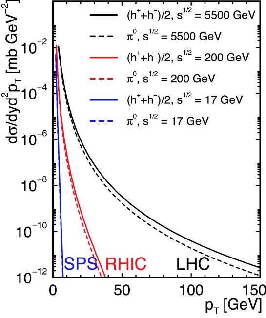
The qualitative statement is clearly confirmed by fig. 9, which shows the transverse-momentum distribution of neutral pions and inclusive charged hadrons predicted by a recent LO pQCD calculation invoking the standard factorized pQCD hadron-production formalism [73] (see section 1 on page 1). The significant hardening of the spectra with $\sqrt{s}$ leads to two important consequences for p–A and A–A collisions (see below): a notably reduced sensitivity to initial state (kinematic) effects, smaller Cronin effect, and larger variation of the final-state effects, such as parton energy loss, with $p_{\mathrm{T}}$.

Another impressive example of the expected hardness of the LHC events is given in table 4 reporting the inclusive, accumulated jet cross section per participant pair, $1/(T_{\rm AB}\sigma^{\rm geo}_{\rm AB})\,\sigma(E_{\mathrm{T}}\geq E_{\mathrm{T}}^{0})$, for jets with $E_{\mathrm{T}}\geq E_{\mathrm{T}}^{0}$ at central pseudo-rapidity ($\left|\eta\right|<0.5$) for various transverse minimum jet energies $E_{\mathrm{T}}^{0}$. At LHC energies, high-$E_{\mathrm{T}}$ jets will be copiously produced in heavy-ion collisions and therefore for the first time experimentally accessible. We shall see in the next section and throughout the next chapter that they are a very profound tool to probe the partonic medium created in such collisions.

5 Hard processes as probes of QGP

Assuming the absence of nuclear and QCD medium effects, a nucleus–nucleus collision can be considered as a superposition of independent NN collisions. Thus, the cross section for hard processes should scale from pp to A–A with the number of inelastic nucleon–nucleon collisions according to binary scaling [74]. The effects modifying the simple scaling with $N_{\rm coll}$ are usually divided in two classes:

• Initial-state effects are effects acting on the hard cross section in a way that depends on the size and energy of the colliding nuclei, but not on the medium formed in the collision, such as Cronin enhancing [75], nuclear shadowing and gluon saturation (described in section 4).

• Final-state effects are effects induced by the created medium that influence the yields and the kinematic distributions of the produced hard partons, such as partonic energy loss. Final-state effects are not correlated to initial-state effects; they depend strongly on the properties of the medium (gluon density, temperature and volume). Therefore, they provide information on these properties.

In order to distinguish the influence of the different effects on the various observables and to draw conclusions, a systematic study of the effects in pp  p–A and A–A is required, such as has recently been undertaken at RHIC [76]. Initial state effects can be studied in pp and p–A collisions and then reliably extrapolated to A–A. If the QGP is formed in A–A collisions, the final state effects will be significantly stronger than what is expected by the extrapolation from p–A. In this context, hard scattering processes are an excellent experimental probe in heavy-ion collisions inasmuch as they posses the following interesting properties:

• They are produced in the early stage of the collision in the primary, short-distance, partonic scattering with large virtuality $Q^{2}$. Thus, owing to the uncertainty relation, their production happens on temporal and spatial scales, $\Delta\tau\sim 1/Q$ and $\Delta r\sim 1/Q$, which are sufficiently small to be unaffected by the properties of the medium (i.e. by final-state effects) and therefore they directly probe the partonic phase of the reaction.

• Because of the large virtuality, their production cross section can be reliably calculated with pQCD (collinear factorization plus Glauber multi-scattering, see section 1 on page 1) or via the Color Glass Condensate (CGC) framework [67]. In fact, since QCD is asymptotically free [77, 78], the running coupling constant (calculated up to two internal loops)

  $$\alpha_{\rm S}(Q^{2})=\frac{1}{b\,L}\,(1-\frac{b^{\prime}}{b}\,\frac{\ln L}{L})\hskip 5.69046pt\text{where}\hskip 5.69046ptL=\ln\frac{Q^{2}}{\Lambda^{2}}$$ (7)

  becomes small for large values of $Q^{2}\gg\Lambda\simeq\Lambda_{\rm QCD}$.  Hence, the higher-order terms (in general, higher than NLO) can be neglected in an expansion of the cross section in powers of $\alpha_{\rm S}$.

• In the absence of medium effects, their cross section in A–A reactions is expected to simply scale with that measured in NN collisions times the number of available point source scattering centres (binary scaling).

• They are expected to be significantly attenuated through the special QCD type energy loss mechanisms, when they propagate inside the medium. The current theoretical understanding of these mechanisms and of the magnitude of the energy loss are extensively covered in the next chapter, with particular focus on the suppression of high-energy jets.

In short, hard probes are perturbative processes testing non-perturbative physics. The input (yields and $p_{\mathrm{T}}$ distributions) is known from the measurements carried out in pp (and p–A) interpolated to the A–A energy by means of pQCD (and typically scaled according to $N_{\rm coll}$). The comparison of the measured outcome, after being influenced by the medium, to the known input allows to extract information of the medium properties. Typical probes include the production of quarkonia and heavy flavours [79], direct photons and photon tagged jets [80], and —as we will see in the next chapter— jet and di-jet production [81] and within limited scope leading-particle $p_{\mathrm{T}}$-spectra.

Chapter 2 Jets in heavy-ion collisions

High-energy jets are sensitive probes of the partonic medium produced in nucleon–nucleon collisions. In fact, they possess all properties listed at the end of the previous chapter:

• Their initial production is not affected by final state effects, because the large value of the virtuality $Q=2\,E_{\mathrm{T}}$ for $E_{\mathrm{T}}\geq 10\leavevmode\nobreak\ \mbox{${\rm GeV}$}$ implies production space-time scales of $\sim 1/(2\,E_{\mathrm{T}})\,{\buildrel<\over{{}_{\sim}}}\,0.01\leavevmode\nobreak\ \mbox{${\rm fm}$}$, which are much smaller than the expected life-time of the partonic phase at the LHC, $\tau\,{\buildrel>\over{{}_{\sim}}}\,10\leavevmode\nobreak\ \mbox{${\rm fm}$}$. Thus, the early-produced partons (from which the jets eventually emerge) will experience the partonic evolution of the collision.

• As a consequence of the large virtuality compared to $\Lambda_{\rm QCD}$, their production cross section measured in pp (or $\mathrm{p\overline{p}}$) and p–A collisions is calculable within the framework of pQCD. If $A^{\frac{1}{3}}\Lambda_{\rm QCD}\ll Q$ and assuming that initial state effects are known and under control the cross section can be safely scaled to nucleus–nucleus collisions. We review the general ideas behind jets physics at hadron colliders in section 1.

• Strong final state effects are expected to influence the propagation of high-energy partons through the medium formed in nucleus–nucleus collisions. Of particular interest is the predicted medium-induced energy loss of the hard partons via gluon radiation in a dense partonic medium. Depending on the hadronization and thermalization lengths of the penetrating probes, see chapter 5, jet tomography will be useful to investigate such phenomena. We summarize the theoretical framework of various ‘jet quenching’ models in section 2.

The experimental situation at RHIC, where for the first time hard processes are experimentally accessible in heavy-ion collisions with sufficiently high rates, is reported in section 3 In section 4 we describe a final state quenching model, which describes most of the high-$p_{\mathrm{T}}$ observables at RHIC.

1 Concepts of jet physics

In the collision of high-energy hadrons one of four different types of scattering reactions can occur: elastic, diffractive, soft-inelastic and hard. Elastic collisions are interactions where the initial and final particles are of the same type and energy. They can be regarded as diffractive processes, but involving the exchange of quantum numbers of the vacuum only. Inelastic diffractive processes are similar, here one or both of the incident hadrons break apart. Soft-inelastic collisions also induce the breakup of the incident hadrons but at rather low momentum transfers. They are best described by exchanges of virtual hadrons (Regge theory) and comprise the largest part of the total cross section.

Figure 1: Illustration of $2$-to-$2$ parton scattering in the hard collision of two incident hadrons. The figure is adapted from LABEL:field2002.

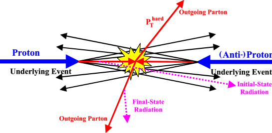
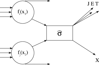
Of particular interest are the hard collisions, visualized in fig. 1, in which the partons within the hadrons (e.g. proton or anti-proton) interact directly. The incident hadrons break apart and many new particles are created. The outgoing partons from the hard sub-process fragment into jets of particles. The rest of the particles in the event are rather soft particles, which mostly arise due to the break up of the remnants of the incident hadrons, and together form the underlying event. The hard-scattering component of the event consists of the outgoing two jets including Initial State Radiation (ISR) and Final State Radiation (FSR). ISR and FSR introduce corrections to the basic $2$-to-$2$ QCD processes, which mimic NLO topologies in Monte Carlo event generators.

(a) Experiment

(b) Monte Carlo

Figure 2: Graphical representation of the evolution of a jet: 2(a) at parton, particle and detector levels in experiments; 2(b) at parton, parton shower and particle levels in Monte Carlo simulations.

By definition, hard collisions involve very large momentum transfers, $Q$, and probe the structure of the hadrons at short distances. As a consequence of asymptotic freedom, the QCD running coupling constant becomes small at this scale ($\alpha_{\rm S}\,{\buildrel<\over{{}_{\sim}}}\,0.3$, see eq. (7) on page 7) and perturbative methods become applicable.

Thus, the measurement of inclusive jet and dijet cross sections, as well as various other jet properties can be used to test the predictions of pQCD, improve the knowledge on $\alpha_{\rm S}$ and PDFs at large $x$ and look for quark compositeness [83].

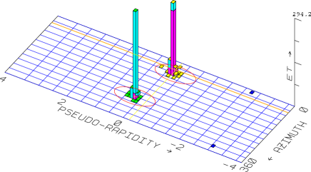
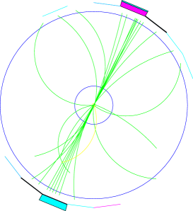
In order to draw comparisons between the data and the theoretical descriptions, jet finding (and defining) algorithms are used at the detector level, as clusters of towers in calorimeters, see fig. 2(a), and in Monte Carlo simulations, as final-state hadrons or outgoing partons from the hard sub-process, see fig. 2(b). A well-defined jet algorithm must not be sensitive to the level of the input it is applied to, as we will outline in section 2. Because perturbative calculations deal only with gluons and quarks, the subsequent jet evolution from partons and in particular the generation of the underlying event typically is performed with Monte Carlo generators. The event generators mimic non-perturbative fragmentation and hadronization processes converting partons into color-confined hadrons. Although, at hadron level, they fail to predict the shape of the measured (differential) jet cross-sections, presented in section 4, they allow to study the performance of the jet finding at the Monte Carlo or —including a realistic detector response simulation— at the (simulated) detector level.

1 Jet production in pQCD

The perturbative component of the hard-scattering cross section, the parton–parton cross section, can be analytically expanded in orders of $\alpha_{\rm S}$, which becomes relatively small for large $Q^{2}$. The contribution of each order to the scattering amplitude conveniently is expressed in the framework of Feynman diagrams.

(a) LO

(b) NLO (UV)

(c) NLO (IR)

Figure 3: Example of some QCD processes at LO and NLO.

Figure 3 shows a few $2$-to-$2$ and $2$-to-$3$ processes contributing to LO ($\alpha_{\rm S}^{2}$) and NLO ($\alpha_{\rm S}^{3}$). The LO diagrams consist of all ways connecting the two incoming partons with the two outgoing partons using the basic QCD interaction vertices and do not include any internal loops. The NLO processes are much more complicated because the diagrams with 2 or 3 partons in the final state have infra-red and ultra-violet divergences. The processes with 3 partons in the final state diverge, if two of the partons become collinear or one of them soft (infra-red divergency). The processes with 2 partons in the final state must have one internal loop introducing another kind of divergent integral. These ultra-violet divergencies are isolated with well-defined regularization schemes (e.g. cut-off or dimensional regularization methods). Introducing the renormalization scale, $\mu_{\rm R}$, the singularities eventually are absorbed into the (bare) parameters of the theory (e.g. coupling, quark masses and vertices), which in turn become dependent on the momentum transfer and renormalization scales (and, at higher orders, also on the regularization scheme). In the massless limit and for suitably defined, inclusive observables the collinear and soft contributions from the real and virtual gluon diagrams cancel after regularization [62].

Since the statistical momentum distributions of the initial hard-scattering partons are known, any cross section involving partons in the initial state is given by the convolution of the PDFs and the partonic cross section summed over all contributing partons and all Bjorken-$x$ values. The factorization of the cross section allows the separation of the long-distance and short-distance physics [84] (see below). The scale, $\mu_{\rm F}$, introduced by the factorization distinguishes the two domains. Both, the PDFs and the partonic cross section, therefore depend on it. Typically, one takes the same value for the factorization scale as for renormalization scale ($\mu_{\rm F}\simeq\mu_{\rm R}$) [85].

Figure 4: The relative contribution of parton–parton sub-processes contributing to the inclusive single-jet cross section at mid-pseudo-rapidity ($\eta_{1}\simeq\eta_{2}\simeq 0$) at $\sqrt{s_{\scriptscriptstyle{{\rm NN}}}}=1.8\leavevmode\nobreak\ \mbox{${\rm TeV}$}$ as a function of the transverse jet energy. The calculation uses $\mu_{\rm F}=E_{\mathrm{T}}/2$ and the CTEQ 4L parameterization for the PDFs.

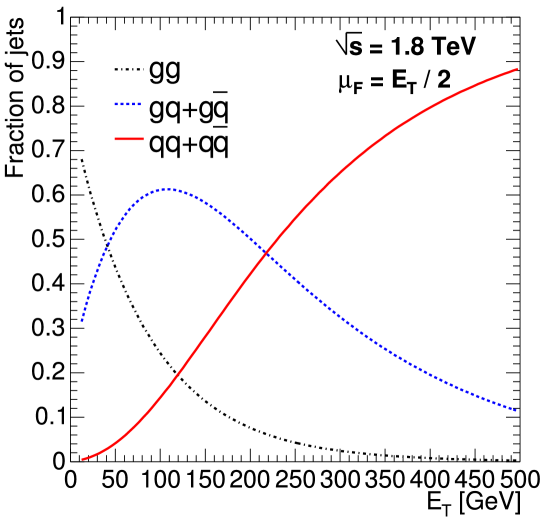
The PDFs, $f_{i}(x,\mu^{2}_{\rm F})$, describe the initial parton momentum of the flavour $i$ ($\mathrm{u}$, $\mathrm{\overline{u}}$, $\mathrm{d}$, $\mathrm{\overline{d}}$, $\mathrm{g}$, etc.) as the fraction $x$ of the incident hadron momentum (explained in section 1 on page 1). To compute the relative contribution of the sub-processes to the partonic cross section we use the CTEQ 4L parameterization. According to eq. (5) on page 5 for jets at mid-pseudo-rapidity $x\simeq x_{\mathrm{T}}=2\,E_{\mathrm{T}}/\sqrt{s_{\scriptscriptstyle{{\rm NN}}}}$ holds. For the factorization scale we take $\mu_{\rm F}=E_{\mathrm{T}}/2$. The resulting contribution for $\sqrt{s_{\scriptscriptstyle{{\rm NN}}}}=1.8\leavevmode\nobreak\ \mbox{${\rm TeV}$}$ based on the type of the incoming partons as a function of the transverse jet energy at mid-pseudo-rapidity is shown in fig. 4. At low $E_{\mathrm{T}}$, jet production is dominated by gluon–gluon ($\mathrm{g}$$\mathrm{g}$) and gluon–(anti-)quark ($\mbox{$\mathrm{g}$}\mbox{$\mathrm{q}$}+\mbox{$\mathrm{g}$}\mbox{$\mathrm{\overline{q}}$}$) scattering. At high $E_{T}$ it is largely quark–(anti-)quark ($\mbox{$\mathrm{q}$}\mbox{$\mathrm{q}$}+\mbox{$\mathrm{q}$}\mbox{$\mathrm{\overline{q}}$}$) scattering. The gluon–(anti-)quark scattering is still about $40$% at $E_{T}=250\leavevmode\nobreak\ \mbox{${\rm GeV}$}$ because of the large color factor associated with the gluon, and significantly contributes to the cross section at all $E_{\mathrm{T}}$ values.

2 Jet defining and finding procedures

The distribution of final state quarks and gluons cannot be measured directly as, due to confinement, the final state objects of the hard-scattering reaction are colorless particles (mostly hadrons). For studies of parton-level interactions, event properties, which only are weakly affected by long distance processes and which closely relate the partonic and hadronic final states, are desirable. The concept of jets and the jet identification algorithms allows to associate the partons and the hadrons observed in final states of high energy collisions, a correspondence referred to as Local Parton-Hadron Duality (LPHD) [86]. If LPHD is satisfied, the study of jets may be regarded as a tool for mapping the observed long-distance hadronic final states onto underlying short-distance partonic states.

(a) Calorimeter

(b) Tracking chamber

Figure 5: Jet event in the CDF calorimeter 5(a) and central tracking chamber 5(b) identified by the cone jet finder, JetClu, with $R=0.7$ (see below). The figure is taken from LABEL:affolder2001.

Although ‘everyone knows a jet, when they see it’, because they stand out by their nature (fig. 5), precise definitions are elusive and detailed. Jet finding algorithms define a functional mapping

$$\mathbf{particles}\stackrel{{\scriptstyle\mathbf{jet\;algorithm}}}{{-\!\!\!-\!\!\!-\!\!\!-\!\!\!-\!\!\!-\!\!\!-\!\!\!-\!\!\!-\!\!\!\longrightarrow}}\mathbf{jets}$$

between the particles in the event, given by their kinematical description (e.g. momenta) and the configuration of jets, represented by suitable jet variables.

Ideally, jet defining algorithms must be [88]

• fully specified: the jet finding procedure, the kinematic variables of the jet and the various corrections should be uniquely and completely defined.

• theoretically well behaved: the algorithm should be infrared and collinear safe, without the need for ad-hoc parameters.

• detector independent: there should be no dependence on detector type, segmentation or size.

• consistent: the algorithm should be equally applicable at the theoretical and experimental levels.

The first two criteria must be fulfilled by every algorithm as LPHD can only be satisfied if the applied jet algorithm is infrared safe. This ensures that its outcome is insensitive to the emission of soft or collinear partons. Therefore, the jet observable must not change by adding an additional particle with $E\rightarrow 0$ to the final state or when replacing a pair of particles by a single particle with the summed momentum. The last two criteria, however, can probably never be totally true, since it is not possible to completely remove dependencies on the experimental apparatus.

Jet kinematics

The interacting partons are not generally in the centre-of-mass frame of the colliding system, because the fraction of the hadron momentum carried by each parton varies from event to event. Therefore, the centre-of-mass system of the partons is randomly boosted along the direction of the colliding hadrons, so that jets are conveniently described by longitudinally boost-invariant variables:

$$\rm{mass}\hskip 99.58464pt m =\sqrt{E^{2}-p_{\mathrm{x}}^{2}-p_{\mathrm{y}}^{2}-p_{\mathrm{z}}^{2}}$$

$$\rm{transverse\leavevmode\nobreak\ momentum}\hskip 11.38092pt p_{\mathrm{T}} =\sqrt{p_{\mathrm{x}}^{2}+p_{\mathrm{y}}^{2}}$$

$$\rm{azimuthal\leavevmode\nobreak\ angle}\hskip 42.67912pt \phi =\arctan\left(p_{\mathrm{y}}/p_{\mathrm{x}}\right)$$

$$\rm{rapidity}\hskip 82.51282pt y ={\rm arctanh}\left(p_{\mathrm{z}}/E\right)=\frac{1}{2}\ln\left(\frac{E+p_{\mathrm{z}}}{E-p_{\mathrm{z}}}\right)\;.$$

In the high energy limit, when $p>>m$, the directly measured quantities conveniently are: energy ($E$) or transverse energy ($E_{\mathrm{T}}=E\,\sin\theta\simeq p_{\mathrm{T}}$), the azimuth ($\phi$) and the pseudo-rapidity

$$\eta=-\ln\left[\tan\left(\theta/2\right)\right]\;,$$

where the polar angle is given by $\theta=\arctan(p_{\mathrm{T}}/p_{\mathrm{z}})$.

Jet algorithms

Even though the criteria listed in section 2 lead to restrictions on possible algorithms, a variety of jet definitions emerged over time (see LABEL:blazey2000 for an overview). They can be grouped into two fundamental classes: recombination (clustering) algorithms [89, 90, 91, 92, 93, 94, 95] and cone algorithms [96, 97, 98, 99, 100, 101, 102]. Both are based on the assumption that hadrons associated with a jet will be ‘nearby’ each other. The definition of cone jets is based on vicinity in real space (angles), whereas the recombination algorithms make use of vicinity in momentum space and, nowadays, go by the name of $k_{\mathrm{T}}$ algorithms.

• The $k_{\mathrm{T}}$ algorithms [93, 94] are inspired by QCD parton showering. The algorithms try to mimic the hadronization processes backwards and successively merge pairs of particles (or rather ‘vectors’) in order of increasing transverse momentum. Typically they contain a parameter, $D$, which controls the termination of merging. By design, they are infra-red and collinear safe to all orders and were developed for precise $\mbox{$\mathrm{e^{+}e^{-}}$}\rightarrow\rm{jets}$ studies (see LABEL:moretti1998 for a recent comparison). However, problems arise when the $k_{\mathrm{T}}$ algorithm is applied at hadron–hadron colliders. This is mostly due to difficulties with the substraction of energy from spectator fragments and from the pile-up of the multiple hadron–hadron interactions. Only recently solutions to these problems have been developed [104, 88]

• The cone algorithms [96, 99, 101] historically developed for jet definition in hadron–hadron collisions group all particles within a cone of radius $R$ in $\eta\times\phi$ space into a single jet. The radius is defined as $R=\sqrt{\Delta\eta^{2}+\Delta\phi^{2}}$, where $\Delta\eta$ and $\Delta\phi$ are the separation of the particles (or partons) in pseudo-rapidity and azimuthal angle (in radians) to the jet axis. The way the grouping procedure operates is such that the center of the cone is aligned with the jet direction. Typically, the algorithm starts with a number of (high energy) seeds, but also seedless implementations exist. As cones may overlap, a single particle could belong to two or more cones. Thus, a procedure is introduced to specify how to split or merge overlapping jets. At the parton level NLO calculations require the addition of an ad-hoc separation parameter, $R_{\rm sep}$, to regulate the clustering of the partons and simulate the role of seeds.

3 Improved Legacy Cone Algorithm

The decision to use a cone finder for the present work is based on the fact that the anticipated huge background (or underlying event) for $\rm{Pb}+\rm{Pb}\rightarrow\rm{jet}+\rm{X}$ at the LHC will spoil the recombination scheme of the $k_{\mathrm{T}}$ algorithms. Furthermore, the $\mathcal{O}(n^{3})$ run-time of the $k_{\mathrm{T}}$ algorithms might be too time-consuming for the online version (trigger) of the jet finder.  Instead, we decided to implement the Improved Legacy Cone Algorithm (ILCA) [88], which has been developed jointly by D0 and CDF before the start of Run II and which is supposed to possess the required features listed on page 5.

The basic idea of the algorithm is to find all of the circles in the $\eta\times\phi$ space (cones in three dimensional space) of a preselected, fixed radius $R$ that contain stable jets. The algorithm starts with an input list of particles, partons or pre-towers, which are grouped into towers according to a simple pre-clustering procedure . Each tower in the event is assigned a massless four-vector $(E_{k}=\left|\vec{p}_{k}\right|,\,\vec{p}_{k})\equiv(E_{k},\phi_{k},\eta_{k})$ pointing into the direction of the tower.

(a) Clustering

(b) Splitting and merging

Figure 6: 6(a) The seedless clustering procedure and 6(b) the splitting-and-merging procedure of the ILCA algorithm. For details see the text.

The jets are defined in three sequential steps:

1. In the clustering procedure, displayed in fig. 6(a), towers belonging to a jet are iteratively accumulated until stable proto-jets are found.

2. In the splitting-and-merging procedure, displayed in fig. 6(b), overlapping jets are split or merged depending on the fraction of energy they share.

3. In the recombination procedure, the kinematical variables of the jets are computed according to a given recombination scheme (e.g. Snowmass, modified Run I or energy scheme, see LABEL:blazey2000).

The clustering method displayed in fig. 6(a) starts by looping over all towers. For each tower $k$, with center $\overrightarrow{k}=\left(\eta_{k},\phi_{k}\right)$, we define a cone of size $R$ centered on the tower

$$\overrightarrow{C_{k}} = \left(\eta_{C_{k}}=\eta_{k},\phi_{C_{k}}=\phi_{k}\right)$$

$$i \in C_{k}\;:\;{\left(\eta_{i}-\eta_{C_{k}}\right)^{2}+\left(\phi_{i}-\phi_{C_{k}}\right)^{2}}\leq R^{2}\;,$$

which contains all towers falling into its circumference.  For each cone we, then, evaluate the $E_{\mathrm{T}}$-weighted average centroid $\overrightarrow{\bar{C}_{k}}=\left(\bar{\eta}_{C_{k}},\bar{\phi}_{C_{k}}\right)$, where

$$\bar{\eta}_{C_{k}}=\frac{\sum_{i\in C_{k}}E_{{\mathrm{T}}_{i}}\eta_{i}}{E_{{\mathrm{T}}_{C_{k}}}}\hskip 14.22636pt\text{and}\hskip 14.22636pt\bar{\phi}_{C_{k}}=\frac{\sum_{i\in C_{k}}E_{{\mathrm{T}}_{i}}\phi_{i}}{E_{{\mathrm{T}}_{C_{k}}}}$$

with its transverse energy content

$$E_{{\mathrm{T}}_{C_{k}}}=\sum_{i\in C_{k}}E_{{\mathrm{T}}_{i}}\;.$$

In general, the centroid $\overrightarrow{\bar{C}_{k}}$ is not identical to the geometric center $\overrightarrow{C_{k}}$ and, thus, the cone is not stable. If the calculated centroid of the cone lies outside of the initial tower, further processing of that cone is skipped and the cone is discarded.  All the cones, which yield a centroid within the original tower, are kept for re-iteration. For these cones the process of calculating a new centroid about the previous centroid is repeated. Thus, the cones are allowed to ‘flow’ away from the original towers. The iteration continues until either a stable cone center is found or the centroid moves out of the fiducial volume. All the surviving stable cones constitute the list of proto-jets. 

Typically, a number of overlapping proto-jets, for which towers are shared by more than one cone, will be found after applying the clustering procedure. These are subject of the splitting-and-merging procedure sketched in fig. 6(b). The suggested algorithm starts with the list of all proto-jets and always works with the highest $E_{\mathrm{T}}$ proto-jet remaining on the list. After a merging or splitting occurred, the $E_{\mathrm{T}}$ ordering on the list of remaining proto-jets can change, since the survivor of merged jets may move up while split jets may move down. Once a proto-jet shares no tower with any of the other proto-jets, it becomes a jet stored on the list of final jets, which is not affected by the subsequent merging and splitting of the remaining proto-jets. The decision to split or merge a pair of overlapping proto-jets is based on the percentage of transverse energy shared by the lower $E_{\mathrm{T}}$ proto-jet. Proto-jets, which share a fraction greater than $f$ (typically $f=50\%$), will be merged; others will be split with the shared towers individually assigned to the proto-jet, which is closest in $\eta\times\phi$ space. The method will perform predictably even in the case of multiply split and merged jets, but there is no requirement that the centroid of the split or merged proto-jet still coincides precisely with its geometric center.

To complete the jet finding process the jet variables have to be computed according to a suitable recombination prescription. Typically, we follow the original Snowmass ($E_{\mathrm{T}}$-) scheme [98]

$$E_{{\rm T}_{J}} = \sum_{i\in J=C}E_{{\rm T}_{i}}$$

$$\eta_{J} = \frac{1}{E_{{\rm T}_{J}}}\sum_{i\in J=C}E_{{\rm T}_{i}}\eta_{i}$$

$$\phi_{J} = \frac{1}{E_{{\rm T}_{J}}}\sum_{i\in J=C}E_{{\rm T}_{i}}\phi_{i}\;,$$ (1)

which simply uses the stable cone variables. That way computing time is reduced, because there is no need to loop over the associated particles (or towers) in the jet, as one would need to do in the energy ($E$-) scheme in order to calculate the jet variables by adding four-vectors of the associated particles (or towers).  As reported by CDF [87], in practice the difference between the two representations is negligible.

4 Inclusive single-jet cross section

The inclusive single-jet cross section can be determined from the process

$$\rm{h}_{1}+\rm{h}_{2}\rightarrow\rm{jet}+\rm{X}$$ (2)

visualized in fig. 7.

Figure 7: Visualization of the jet production process in a hadron–hadron collision. The PDFs give the probability to pick up a certain parton with momentum fraction $x$ of the hadron momentum. The elementary parton–parton interaction can be calculated in pQCD.

In the framework of QCD improved parton model, which we partially have outlined above, the corresponding cross section writes as 

$$\sigma_{\rm jet}=\sum_{i,j}\int\mathrm{d}x_{1}\mathrm{d}x_{2}\,f_{i}(x_{1},\mu^{2}_{F})\,f_{j}(x_{2},\mu^{2}_{\rm F})\,\hat{\sigma}_{ij}[x_{1}P,x_{2}P,\alpha_{\rm S}(\mu_{\rm R}^{2}),\frac{Q^{2}}{\mu_{\rm R}^{2}},\frac{Q^{2}}{\mu_{\rm F}^{2}}]$$ (3)

where, for simplicity, we omit the notation of parton evolution and fragmentation processes, as well as the jet finding procedure at the hadron (or parton) level. The short-distance, two-body parton-level cross section, $\hat{\sigma}_{ij}$, is a function of the momentum carried by each of the incident partons ($x_{1}P$ and $x_{2}P$), the strong coupling $\alpha_{\rm S}(\mu^{2}_{\rm R})$, and the ratio of the renormalization and factorization scales, $\mu^{2}_{\rm R}$ and $\mu^{2}_{\rm F}$, to the characteristic scale of the hard interaction, $Q^{2}$. The LO calculation includes only the contribution of tree-level diagrams for the 2$\rightarrow$2 scattering processes given in Refs. [105, 62]. The NLO calculation adds the diagrams which describe the emission of a gluon as an internal loop and as a final state parton [106, 107, 108, 109, 110, 111]. The scales $\mu_{\rm R}$ and $\mu_{\rm F}$ are intrinsic parameters in a fixed order perturbation theory. In what follows, they are set equal, $\mu_{\rm F}=\mu_{\rm R}\equiv\mu$. Although the choice of the $\mu$ scale is arbitrary, a reasonable value is related to a physical observable, such as the $E_{\mathrm{T}}$ of the jets. 

However, since it is impossible to measure the total jet cross section, one obtains the predictions for the jet cross section as a function of $E_{\mathrm{T}}$ from the general expression, eq. (3), using

$$\frac{E\mathrm{d}^{3}\sigma}{\mathrm{d}p^{3}}\equiv\frac{\mathrm{d}^{3}\sigma}{\mathrm{d}p_{\mathrm{T}}^{2}\mathrm{d}y}=\frac{1}{2\pi E_{T}}\frac{\mathrm{d}^{2}\sigma}{\mathrm{d}E_{\mathrm{T}}d\eta}\;,$$ (4)

where (as often done in jet calculations) the mass of the partons has been assumed to be zero ($p_{\mathrm{T}}=E_{\mathrm{T}}$). Experimentally, the inclusive (differential) jet cross section is defined as the number of jets in a bin of $E_{\mathrm{T}}$ normalized by acceptance and integrated luminosity. All the jets in each event falling within the acceptance region contribute to the cross section measurement as appropriate for an inclusive quantity. Usually, measurements are performed in the central pseudo-rapidity interval ($\left|\eta\right|<1$) and results are averaged in the $\eta$-interval.

Figure 8: Inclusive single-jet cross section from Run I at $\sqrt{s}=1.8\leavevmode\nobreak\ \mbox{${\rm TeV}$}$ for $0.1<|\eta|<0.7$ as published by CDF. The jets are identified with JetClu at $R=0.7$. The data from Run 1A (92-93) and Run 1B (94-95) are compared to the NLO calculation of EKS used with the CTEQ 4M at $\mu=E_{\mathrm{T}}/2$ and a parton-separation value of $R_{\rm sep}=1.3$. The figure is adapted from LABEL:affolder2001.

(a) CDF measurement

(b) D0 measurement

Figure 9: Inclusive single-jet cross section from Run II at $\sqrt{s}=1.96\leavevmode\nobreak\ \mbox{${\rm TeV}$}$. 9(a) The CDF measurement (preliminary) using JetClu with $R=0.7$ is compared to EKS with CTEQ 6.1 at $\mu=E_{\mathrm{T}}/2$ and $R_{\rm sep}=1.3$. The figure is adapted from LABEL:latino2004. 9(b) The D0 measurement (preliminary) using ILCA with $R=0.7$ is compared to JETRAD with CTEQ 6M at $\mu=P^{\mathrm{max}}_{\mathrm{T}}/2$ and $R_{\rm sep}=1.3$. The figure is adapted from LABEL:padley2004.

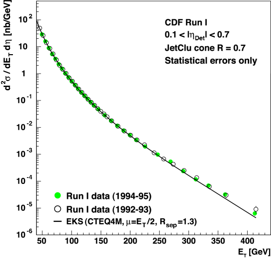
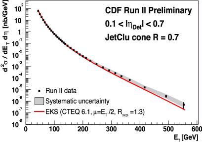
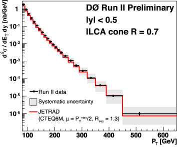
Figure 8 shows the measurement of the inclusive single-jet cross section at $\sqrt{s}=1.8\leavevmode\nobreak\ \mbox{${\rm TeV}$}$ for $0.1<|\eta|<0.7$ as a function of $E_{\mathrm{T}}$ from CDF at the Tevatron $\mathrm{p\overline{p}}$ collider [87]. The jets are identified with a cone finder, called JetClu [99], using a radius of $R=0.7$. The measured and corrected differential cross section is compared to a NLO pQCD calculation of the EKS program [100]. The calculation computes the spectrum at the parton level and uses the NLO CTEQ 4M PDFs at $\mu=E_{\mathrm{T}}/2$ and a parton separation value of $R_{\rm sep}=1.3$. The systematic errors not shown in the figure range between $20$–$50\%$ at high energy. Experimentally the uncertainty is dominated by the uncertainty associated with the Monte Carlo production of realistic jets and underlying events for the derivation of corrections needed to compare the measured cross section at hadron level with calculations at parton level. The theoretical uncertainty is dominated by uncertainty in the PDFs, mainly at high-$x$. The experimental and theoretical developments, thus, are correlated, since the corrections to the raw data depend on detailed modeling of the events, which in turn depends on data quality and size.

Very recently, preliminary results from Run II at Tevatron became available confirming and extending the precise measurements of Run I to higher $E_{\mathrm{T}}$. The preliminary results for the inclusive (differential) single-jet cross section at $\sqrt{s}=1.96\leavevmode\nobreak\ \mbox{${\rm TeV}$}$ by CDF [114] and D0 [113] are shown in fig. 9. The CDF measurement is performed using the Run I cone finder JetClu with $R=0.7$ for the definition of jets at the hadron level, whereas the D0 result has been obtained with the improved Run II cone finder (ILCA) with $R=0.7$. Both are compared to NLO pQCD calculations, EKS with CTEQ 6.1 and JETRAD with CTEQ 6M, respectively. The consistency between the data and the theoretical prediction over many orders of magnitude is remarkable Still, the main source for errors is attributed to the uncertainty in the gluon PDF arising at about $x\,{\buildrel>\over{{}_{\sim}}}\,0.1$, where the new data will provide new constraints for the gluon PDF [115].

5 Jet fragmentation

The single-jet cross section presented in the last section in fig. 8 and fig. 9 is consistent with theoretical predictions at parton level. This is due to LPHD and the way jet finding algorithms are constructed (see section 2). However, the fixed order calculations cannot predict details of the jet structure observed in experiments. Monte Carlo programs implement the parton shower approach approximating higher order QCD processes followed by hadronization. General purpose generators, like HERWIG [116, 117, 118] and PYTHIA [119, 120, 121], provide a variety of elementary $2$-to-$2$ processes. After the leading order calculation the primary hard partons develop into multi-parton cascades or showers by multiple gluon bremsstrahlung. These cascades are based on soft and collinear approximations to the QCD matrix elements and distribute the energy fractions according to the DGLAP parton-evolution equations. The parton shower stops, when the virtuality of the initial parton falls below a cut-off parameter, $Q_{0}\simeq 1\mbox{${\rm GeV}$}>\Lambda_{\rm QCD}$. The non-perturbative evolution is then phenomenologically described by hadronization models like the cluster or string model, which turn the final state partons into hadrons locally distributed in phase space [122, 123]. Due to the cut-off the hadronization process is independent of the hard scattering and the development of the parton shower.

Opposed to hadronization, for which at present only models exist, the evolution of parton showers and the scaling of inclusive fragmentation into hadrons can be described by pQCD. The total fragmentation function for hadrons of type $\rm h$ in a certain process, typically $\mathrm{e^{+}e^{-}}$ annihilation, is defined by

$$F_{\rm h}(x,s)=\frac{1}{\sigma_{\rm tot}}\frac{\mathrm{d}\sigma}{\mathrm{d}x}(\mbox{$\mathrm{e^{+}e^{-}}$}\rightarrow\rm{hX})\;,$$

where $x=2E_{\rm h}/\sqrt{s}$ is the scaled hadron energy in the centre-of-mass frame. The total fragmentation function can be decomposed into a sum of contributions arising from the different primary partons

$$F_{\rm h}(x,s)=\sum_{i}\int_{x}^{1}\frac{\mathrm{d}z}{z}\,C_{i}(z,\alpha_{\rm S}(s))\,D_{{\rm h}/i}(x/z,s)\;,$$

where $C_{i}$ are the coefficients for the particular process and $D_{{\rm h}/i}(x,s=Q^{2})$ are the Fragmentation Functions for turning the parton $i$ into the hadron $\rm h$. Like the PDFs, to leading order, the FFs have an intuitive probabilistic interpretation. Namely, they quantify the probability that the parton $i$ produced at short distance of $1/Q$ forms a jet that includes the hadron $\rm h$ with (longitudinal) momentum fraction $x$ of $i$. Furthermore, they are universal in a sense that they are believed not to depend on the particular processes from which they are derived [124].

(a) Charged hadrons at $Q=5\leavevmode\nobreak\ \mbox{${\rm GeV}$}$

(b) $D(x,100^{2}\leavevmode\nobreak\ \mbox{${\rm GeV}$}^{2})/D(x,5^{2}\leavevmode\nobreak\ \mbox{${\rm GeV}$}^{2})$

(c) Neutral pions at $Q=5\leavevmode\nobreak\ \mbox{${\rm GeV}$}$

(d) $D(x,100^{2}\leavevmode\nobreak\ \mbox{${\rm GeV}$}^{2})/D(x,5^{2}\leavevmode\nobreak\ \mbox{${\rm GeV}$}^{2})$

Figure 10: KKP FFs for gluons and light quarks. 10(a) Fragmentation into charged hadrons at $Q=5\leavevmode\nobreak\ \mbox{${\rm GeV}$}$ and 10(b) the ratio $D(x,100^{2}\leavevmode\nobreak\ \mbox{${\rm GeV}$}^{2})/D(x,5^{2}\leavevmode\nobreak\ \mbox{${\rm GeV}$}^{2})$. 10(c) Fragmentation into neutral pions at $Q=5\leavevmode\nobreak\ \mbox{${\rm GeV}$}$ and 10(d) the ratio $D(x,100^{2}\leavevmode\nobreak\ \mbox{${\rm GeV}$}^{2})/D(x,5^{2}\leavevmode\nobreak\ \mbox{${\rm GeV}$}^{2})$.

The FFs themselves cannot be calculated by pQCD, but as for the PDFs their scaling violation in $s=Q^{2}$ is described in the DGLAP framework according to

$$s\frac{\partial}{\partial s}\,D_{{\rm h}/i}(z,s)=\sum_{j}\int_{x}^{1}\frac{\mathrm{d}z}{z}\,P_{j\,i}(z,\alpha_{\rm S}(s))\,D_{{\rm h}/j}(x/z,s)\;,$$

where the perturbatively calculable splitting functions $P_{j\,i}$ give the evolution of parton $i$ into $j$ [62]. Therefore, the FFs can be parameterized at some fixed scale, typically of the order of a few ${\rm GeV}$, and then predicted at other scales. Several parameterizations of the FFs have been developed performing global NLO fits to the available $\mathrm{e^{+}e^{-}}$ annihilation data from LEP and $ep$ data from HERA [125, 126, 127].

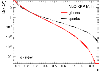
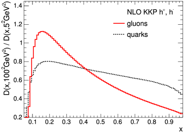
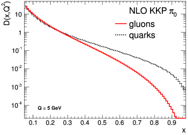
In fig. 10 we show the KKP parameterization [126] at NLO evaluated at the scale of $Q=5\leavevmode\nobreak\ \mbox{${\rm GeV}$}$ and the ratio $D(x,100^{2}\leavevmode\nobreak\ \mbox{${\rm GeV}$}^{2})/D(x,5^{2}\leavevmode\nobreak\ \mbox{${\rm GeV}$}^{2})$ as a function of $x$ for the fragmentation of light quarks and gluons into charged hadrons and neutral pions. The KKP parameterization is obtained by fits to available $\mathrm{e^{+}e^{-}}$ annihilation data performed within $0.1\leq x\leq 1$ in order to avoid mass and non-perturbative effects. As can be seen, on average, quarks tend to fragment harder than gluons, an effect which increases with increasing fragmentation scale.

(a) Jet fragmentation functions

(b) Fraction of jet energy in particles

Figure 11: Jet fragmentation properties measured at mid-pseudo-rapidity comparing CDF-FF (tuned ISAJET to CDF data) and HERWIG fragmentation functions. 11(a) The associated, charged, particle $p_{\mathrm{T}}$-spectrum normalized by the jet energy for different jet energies. 11(b) Fraction of jet energy in associated particles of different $p_{\mathrm{T}}$ for $E_{\mathrm{T}}=100\leavevmode\nobreak\ \mbox{${\rm GeV}$}$ jets. Both figures are taken from LABEL:affolder2001.

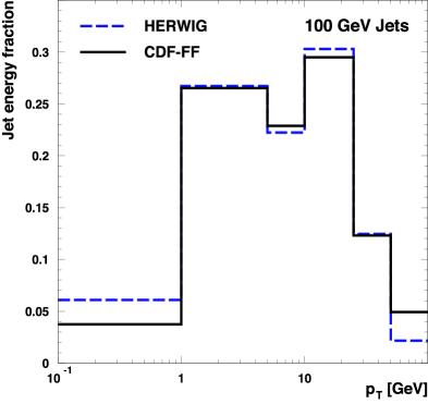
The $p_{\mathrm{T}}$-spectrum of charged particles in a jet has been obtained by CDF using tracking information. The (normalized) distribution, $1/N_{\rm jets}\mathrm{d}N/\mathrm{d}z$, where $z=p_{\mathrm{T}}/E_{\mathrm{T}}^{\rm jet}$, can be regarded as an estimator for the jet FF. The distribution is shown in fig. 11(a) for different jet energies. The fragmentation function of ISAJET (Feynman-Field fragmentation) tuned to give good agreement with data is called CDF-FF. It is compared to HERWIG, which uses cluster/string fragmentation adjusted to LEP data. The change in the cross section, eq. (4), when HERWIG FFs were used instead of CDF-FF, is smaller than the uncertainty attributed to fragmentation functions in general, about $30$ % [87]. For jets with $E_{\mathrm{T}}=100\leavevmode\nobreak\ \mbox{${\rm GeV}$}$ we reproduce in fig. 11(b) the fraction of jet energy carried by associated particles in the jet as a function of $p_{\mathrm{T}}$; again both models are agree. Most of the jet energy is contained in particles of about $1$ to $30\leavevmode\nobreak\ \mbox{${\rm GeV}$}$. On average one third of the jet energy is manifested within the leading particle; a measured fact which is confirmed up to jet energies of $E_{\mathrm{T}}=400\leavevmode\nobreak\ \mbox{${\rm GeV}$}$ [87].

6 Jet properties

The internal structure of jets is dominated by multi-gluon emissions from the primary final-state partons. It is sensitive to the relative quark- and gluon-jet fraction and receives contributions from soft-gluon initial-state radiation and beam–beam remnant interactions. The structure is characterized by jet-shape observables, which must be collinear and infra-red safe. The study of jet shapes provides a stringent test of QCD predictions and validates the models for parton cascades and soft-gluon emissions in hadron–hadron collisions.

Jet shapes may be characterized in differential, $\rho(r)$, and integrated form, $\Psi(r)$, where $r$ is a particle’s radial distance from the jet axis. They are defined as the average fraction of the jet transverse energy (or momentum) that lies inside an annulus or cone concentric to the jet axis in the plane defined by the pseudo-rapidity ($\eta$) and azimuth ($\phi)$. For an annulus of thickness $\Delta r$ and a cone of radius $R$ the differential distribution containing $N_{\rm jets}$ is defined as

$$\rho(r)=\frac{1}{\rm N_{\rm jets}}\sum_{\rm jets}\frac{E^{\mathrm{jet}}_{\mathrm{T}}(r-\frac{\Delta r}{2},r+\frac{\Delta r}{2})}{E^{\mathrm{jet}}_{\mathrm{T}}(0,R)}\hskip 8.5359pt\text{for}\hskip 8.5359pt0\leq r\leq R\;.$$ (5)

The corresponding integrated distribution reads

$$\Psi(r)=\frac{1}{\rm N_{\rm jets}}\sum_{\rm jets}\frac{E^{\mathrm{jet}}_{\mathrm{T}}(0,r)}{E^{\mathrm{jet}}_{\mathrm{T}}(0,R)}\hskip 8.5359pt\text{for}\hskip 8.5359pt0\leq r\leq R\;.$$ (6)

(a) Differential shape

(b) Integrated shape

Figure 12: Differential 12(a) and integrated 12(b) shapes measured by CDF (preliminary) compared to PYTHIA (Tune A) and HERWIG. The jets are defined using the MidPoint algorithm with a cone size of $R=0.7$. The figure is taken from LABEL:cdfpub.

(a) Data versus Monte Carlo generators

(b) Data versus parton contribution (Tune A)

Figure 13: The fraction of the jet transverse momentum outside $r=0.3$ as a function of $P^{\mathrm{jet}}_{\mathrm{T}}$ measured by CDF (preliminary). The jets are defined using the MidPoint algorithm with a cone size of $R=0.7$. 13(a) The measured shape compared to simulations of HERWIG and PYTHIA (default, Tune A and without multiple parton interactions). 13(a) The measured shape compared to calculations of PYTHIA (Tune A) and the separated contributions from quark- and gluon-jets. Both figures are taken from LABEL:martinez2004.

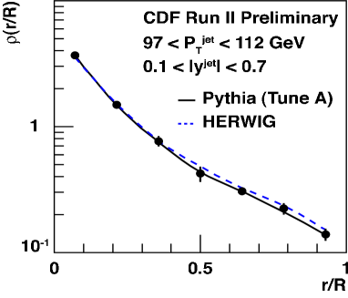
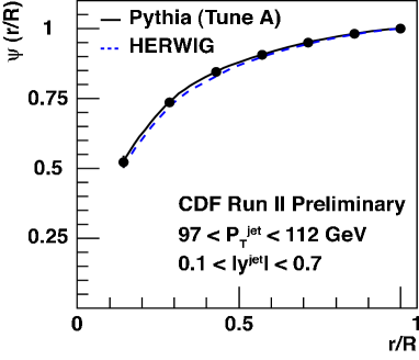
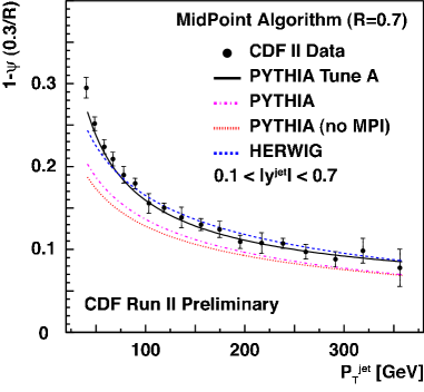
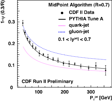
The CDF experiment has presented preliminary results on jet shapes for central jets ($0.1\leq y\leq 0.7$) with transverse momentum $37\leavevmode\nobreak\ \mbox{${\rm GeV}$}\leq P^{\mathrm{jet}}_{\mathrm{T}}\leq 380\leavevmode\nobreak\ \mbox{${\rm GeV}$}$, where jets are searched using the MidPoint algorithm with a cone size of $R=0.7$ [128].  The measured jet shapes of which we show $97\leq P^{\mathrm{jet}}_{\mathrm{T}}\leq 112\leavevmode\nobreak\ \mbox{${\rm GeV}$}$ in fig. 12, have been compared to calculations from PYTHIA (with special parameters, Tune A [130], see below) and HERWIG. Above $P^{\mathrm{jet}}_{\mathrm{T}}\geq 55\leavevmode\nobreak\ \mbox{${\rm GeV}$}$, both the tuned PYTHIA and HERWIG describe the data well, while below HERWIG slightly deviates from the data.

Figure 13 presents, for a fixed radius $r_{0}=0.3$, the average fraction of the jet transverse momentum outside $r=r_{0}$, given by $1-\Psi(r_{0}/R)$, as a function of $P^{\mathrm{jet}}_{\mathrm{T}}$. The preliminary measurements show that the fraction of jet transverse momentum at a given fixed $r_{0}/R$ increases ($1-\Psi(r_{0}/R)$ decreases) with $P^{\mathrm{jet}}_{\mathrm{T}}$. This indicates that the jets become narrower as $P^{\mathrm{jet}}_{\mathrm{T}}$ increases. As can be seen from fig. 13(a) the tuned version of PYTHIA describes all of the data well, whereas HERWIG produces jets that are too narrow at $P_{T}^{\rm jet}\leq 55\leavevmode\nobreak\ \mbox{${\rm GeV}$}$. In order to illustrate the importance of proper modeling of soft-gluon radiation in describing measured jet shapes, in addition to the tuned PYTHIA, two other PYTHIA parameter sets have been compared using default options with and without the contribution from multiple parton interactions between the remnants. PYTHIA with default parameters produces jets systematically narrower than the data throughout the whole $P_{T}^{\rm jet}$ region. Looking at the difference between PYTHIA and PYTHIA without MPI the contribution from secondary parton interactions between remnants to the predicted jet shapes is relatively small and decreases as $P_{T}^{\rm jet}$ increases. Figure 13(b) shows the contributions of gluon and quark jets in PYTHIA (Tune A) compared to the measurement of $1-\Psi(0.3/R)$ as a function of $P^{\mathrm{jet}}_{\mathrm{T}}$.  The Monte Carlo predictions indicate that the measured jet shapes are dominated by contributions from gluon-initiated jets at low $P^{\mathrm{jet}}_{\mathrm{T}}$, while contributions from quark-initiated jets become important at high $P^{\mathrm{jet}}_{\mathrm{T}}$. This can be explained in terms of the different partonic contents in the incident hadrons (proton and anti-proton) in the low- and high-$P^{\mathrm{jet}}_{\mathrm{T}}$ regions, since the mixture of gluon- and quark-jet in the final state partially reflects the nature of the incoming partons that participate in the hard interaction (see fig. 4).

2 Medium-induced parton energy loss

In the first formulation of parton energy loss Bjorken predicted that high energy partons propagating through the QGP suffer differential energy loss due to elastic scattering with the quarks and gluons in the plasma [131]. He further pointed out that as an interesting signature events may be observed, in which the hard collisions may occur such that one jet is escaping without absorption, whereas the other is fully absorbed in the medium. The resulting, collisional, loss was estimated to be $\mathrm{d}E/\mathrm{d}x\simeq\alpha_{\rm S}^{2}\sqrt{\varepsilon}$, where $\varepsilon$ is the energy density of the (ideal) QGP. The loss turns out to be quite low, of the order of $0.1\leavevmode\nobreak\ \mbox{${\rm GeV}$}/\mbox{${\rm fm}$}$ [132].

However, QCD gluon bremsstrahlung, as in QED bremsstrahlung, is another important —if not the dominant— source of energy loss [133, 134]. Due to multiple inelastic scattering and induced gluon radiation high-energy jets and high-$p_{\mathrm{T}}$ leading hadrons become depleted, quenched [135] or even extinct. The radiative loss, as we will report in the following, is considerably larger than the collisional loss. A number of theoretical studies have dealt with the subject [136, 137, 138, 139, 140, 141, 142, 143, 144, 145, 146, 147, 148, 149, 150]. 

In the next section we briefly present the general ideas of the model proposed by Baier-Dokshitzer-Mueller-Peigné-Schiff–Zakharov (BDMPS-Z) [137, 138, 141] and its evaluation in the framework of quenching probabilities (weights) [154] for light quarks and gluons, as calculated by Salgado and Wiedemann [155].

1 Medium-induced radiative energy loss

It has been shown [136] that the genuine pQCD process, depicted in fig. 14, dominantly determines the energy loss of an energetic parton traversing through dense QCD matter.

Figure 14: Typical gluon-radiation diagram, adapted from LABEL:baier2002.

After its initial production in a hard collision the energetic parton with energy $E$ radiates off a gluon with energy $\omega$ with a probability proportional to $L$, the size of the dense medium it traverses. Due to its non-abelian nature the radiated gluon, itself, subsequently suffers multiple scattering due to the interactions in the medium with a mean free path $\lambda$, which decreases as the density of the medium increases. The number of scatterings with momentum transfer $q^{2}_{\rm T}$ that the radiated gluon undergoes until it eventually decoheres, is proportional to $L$, too. Thus, the average energy loss of the parton must be proportional to $L^{2}$.  This is the most distinctive feature of the QCD energy loss compared to the QED case being only proportional to $L$. It arises due to the non-abelian character of QCD: the fact that gluons interact with each other, while photons do not. Note that we concentrate on the coherent regime of the Landau-Pomeranchuk-Migdal (LPM) effect valid for intermediate values of $\omega$,

$$\omega_{\rm BH}\sim\lambda\,q^{2}_{\rm T}\ll\omega\ll\omega_{\rm fact}\sim L^{2}\,q^{2}_{\rm T}/\lambda\leq E\rightarrow\infty\;,$$

in-between the Bethe-Heitler and factorization regimes [136, 137].

Conveniently, the properties of the medium are collectively encoded in the transport coefficient, $\hat{q}$, of the medium, which is defined as the average medium-induced transverse momentum squared transferred to the projectile per mean free path,

$$\hat{q}=\frac{\left<q_{\rm T}^{2}\right>}{\lambda}\;.$$ (7)

The scale of the radiated energy distribution $\omega\,\mathrm{d}I/\mathrm{d}\omega$ (or $\omega\,\mathrm{d}^{2}I/\mathrm{d}\omega\mathrm{d}k_{\mathrm{T}}$) is set by the characteristic energy

$$\omega_{\rm c}=\frac{1}{2}\,\hat{q}\,L^{2}$$ (8)

of the emitted gluon, which depends on the in-medium path-length of the projectile and on the transport coefficient of the medium.

In the original BDMPS-Z calculation [137, 138, 141] the radiated gluon is allowed to exploit the full transverse phase space regardless of its energy. However, physically the transverse momentum $k_{\rm T}$ of the radiated gluon is kinematically bound to be smaller than its energy $\omega$. This imposes a constraint on the emission probability via the dimensionless quantity

$$R=\omega_{\rm c}\,L\,=\frac{1}{2}\,\hat{q}\,L^{3}$$ (9)

first introduced as ‘density parameter’ in LABEL:salgado2002.

Figure 15: The medium-induced radiated gluon energy distribution $\omega\,\mathrm{d}I/\mathrm{d}\omega$ for different values of the kinematical constraint $R=\omega_{\rm c}\,L$ and in the original form of BDMPS-Z (for $R\rightarrow\infty$). The figure is taken from LABEL:salgado2003.

In the multiple scattering approximation of the inclusive radiation spectrum LABEL:salgado2003, referred to as BDMPS-Z-SW, the two parameters $\omega_{\rm c}$ and $R$ determine the energy distribution of radiated gluons, $\omega\,\mathrm{d}I/\mathrm{d}\omega$, reproduced in fig. 15. While $\omega_{\rm c}$ sets the scale of the distribution, $R$ controls its shape in the region $\omega\ll\omega_{\rm c}$ suppressing soft-gluon emission through the kinematical bound on $k_{\rm T}$ ($k_{\rm T}<\omega$). The BDMPS-Z case corresponds to $R\to\infty$. It can be recovered by considering an infinitely-extended medium: taking $L\to\infty$ for fixed finite $\omega_{\rm c}$. In the limit $R\to\infty$ the distribution is of the form

$$\lim_{R\to\infty}\omega\frac{\mathrm{d}I}{\mathrm{d}\omega}\simeq\frac{2\,\alpha_{\rm S}\,C_{\rm R}}{\pi}\left\{\begin{array}[]{lll}\sqrt{\frac{\omega_{\rm c}}{2\omega}}&{\rm for}&\omega<\omega_{\rm c}\\ \frac{1}{12}\,\left(\frac{\omega_{\rm c}}{\omega}\right)^{2}&{\rm for}&\omega\geq\omega_{\rm c}\\ \end{array}\right.$$ (10)

where $C_{\rm R}$ is the QCD coupling factor or Casimir factor between the considered hard parton and the gluons in the medium; it is $C_{\rm F}=4/3$ if the parton is a quark and $C_{\rm A}=3$ if the parton is a gluon.

In the eikonal limit of very large parton initial energy $E$ ($E\gg\omega_{\rm c}$), the integral of the radiated-gluon energy distribution estimates the average energy loss of the parton

$$\left<\Delta E\right>_{R\to\infty}=\lim_{R\to\infty}\int_{0}^{\infty}\omega\frac{\mathrm{d}I}{\mathrm{d}\omega}\,\mathrm{d}\omega\propto\alpha_{\rm S}\,C_{\rm R}\,\omega_{\rm c}\propto\alpha_{\rm S}\,C_{\rm R}\,\hat{q}\,L^{2}\;.$$ (11)

Note that, due to the steep fall-off at large $\omega$ in eq. (10), the integral is dominated by the region $\omega<\omega_{\rm c}$. The average energy loss is:

• proportional to $\alpha_{\rm S}$ (typically we take $0.3$ instead of $0.5$);

• proportional to $C_{\rm R}$ and, thus, larger by a factor $9/4$ for gluons than for quarks;

• proportional to the transport coefficient of the medium;

• proportional to $L^{2}$;

• independent of the parton initial energy $E$.

It is a general peculiarity of all calculations [136, 137, 138, 139, 140, 141, 142, 143, 144, 145, 146, 147, 148, 149, 150] that the radiated energy distribution eq. (10) in the LPM regime does not depend on energy $E$ of the initial parton. However, depending on the way various kinematic bounds are taken into account, the resulting $\Delta E$ is $E$-independent [137, 138, 141] or depends logarithmically on $E$ [148, 149, 150]. In any case, there is always strong intrinsic dependence of the radiated energy on the initial energy, simply determined by the fact that the former cannot be larger than the latter, $\Delta E\leq E$, as we will further discuss in section 2.

The transport coefficient can be related to the density $\rho$ of the scattering centers and to the typical momentum transfer in the gluon scattering off these centers, $\hat{q}=\rho\,\int q^{2}\mathrm{d}\sigma/\mathrm{d}q^{2}$. For cold nuclear matter

$$\hat{q}_{\rm cold}\simeq 0.05\leavevmode\nobreak\ \mbox{${\rm GeV}$}^{2}/\mbox{${\rm fm}$}\simeq 8\,\rho_{0}$$

has been obtained using the nuclear density $\rho_{0}=0.16\leavevmode\nobreak\ \mbox{${\rm fm}$}^{-3}$, the gluon PDF of the nucleon and $\alpha_{\rm S}=0.5$ [137, 138]. The value agrees with the extracted value $\hat{q}=(9.4\pm 0.7)\,\rho_{0}$ resulting from the analysis of gluon $k_{\rm T}$-broadening in experimental data of J/$\psi$ transverse-momentum distributions [158]. The estimation for a hot medium [137, 138]

$$\hat{q}_{\rm hot}\simeq 1\leavevmode\nobreak\ \mbox{${\rm GeV}$}^{2}/\mbox{${\rm fm}$}\simeq 20\,\hat{q}_{\rm cold}$$ (12)

based on perturbative treatment ($\alpha_{\rm S}=0.3$) of gluon scattering in an ideal QGP with a temperature of $T\simeq 250\leavevmode\nobreak\ \mbox{${\rm MeV}$}$ resulted in the value of the transport coefficient of about a factor twenty larger than for cold matter. The average energy loss of the cold and hot medium according to eq. (11) amounts to

$$\Delta E_{\rm cold}\approx 0.02\,\mbox{${\rm GeV}$}\,(L/\mbox{${\rm fm}$})^{2}\hskip 14.22636pt\text{and}\hskip 14.22636pt\Delta E_{\rm hot}\approx 0.3\,\mbox{${\rm GeV}$}\,(L/\mbox{${\rm fm}$})^{2}\;.$$

The precise values must not be taken too serious. However, the large difference suggests that the hot matter is may be rather effective in stimulating the energy loss. The reason is due to

• the higher density of color charges and the correspondingly shorter mean free path of the probe in the QGP;

• the fact that deconfined gluons have harder momenta than confined gluons and, therefore, the typical momentum transfers are larger.

Figure 16: Transport coefficient as a function of energy density for different media: cold matter, massless hot pion gas and ideal QGP. The figure is adapted from LABEL:baier2002.

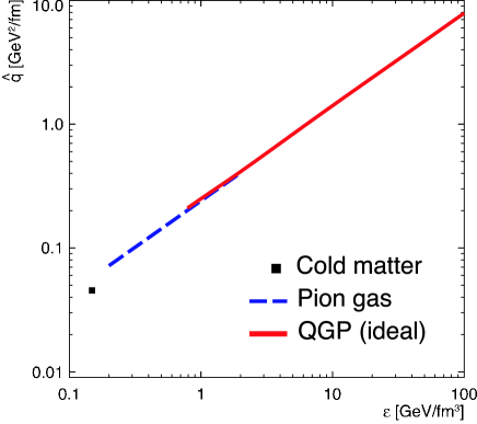
Figure 16 shows the estimated dependence of the transport coefficient, $\hat{q}$, on the energy density, $\varepsilon$, for different equilibrated media (cold matter, hot pion gas and ideal QGP) [156]. Assuming that the QGP is formed (and sustained) at the LHC around $\varepsilon\simeq 100\leavevmode\nobreak\ \mbox{${\rm GeV}$}/\mbox{${\rm fm}$}^{3}$, one expects a transport coefficient of the order of $\hat{q}\simeq 10\leavevmode\nobreak\ \mbox{${\rm GeV}$}^{2}/\mbox{${\rm fm}$}$.

So far, we have assumed a static medium (with a constant transport coefficient). Though, due to the expansion of the system, the density of the medium decreases strongly in time. Hence, the transport coefficient should be time-dependent. However, it turns out [159, 155] that a simple scaling law exists, which translates the gluon energy distribution for an expanding medium with a time-decreasing $\hat{q}(\xi)$ into an equivalent distribution for a static medium, with $\left<\hat{q}\right>=\mathrm{const}$, via

$$\left<\hat{q}\right>=\frac{2}{L^{2}}\,\int_{\xi_{0}}^{L+\xi_{0}}\left(\xi-\xi_{0}\right)\,\hat{q}(\xi)\,\mathrm{d}\xi\;,$$ (13)

where $\xi_{0}\sim 0.1\leavevmode\nobreak\ \mbox{${\rm fm}$}\ll L$ is the time, at which the parton is produced. Thus, depending on how one implements the expansion dynamics (e.g.  one-dimensional Bjorken expansion) one can translate the values for time-averaged into time-dependent transport coefficients.

2 Quenching weights

The spectrum of the additional medium-induced energy loss due to scattering in spatially-extended QCD matter can be characterized by the probability $P(\Delta E)$ that the radiated gluons carry altogether the energy $\Delta E$. Assuming the independent emission of soft gluons from the hard parton, the corresponding ansatz in the soft limit ($\Delta E\ll E$) reads

$$P(\Delta E)=\sum_{n=0}^{\infty}\left[\prod_{i=1}^{n}\int\mathrm{d}\omega_{i}\,\frac{\mathrm{d}I(\omega_{i})}{\mathrm{d}\omega}\right]\,\delta(\Delta E-\sum_{i=0}^{n}\omega_{i})\,\exp{\left[-\int\mathrm{d}\omega\,\frac{\mathrm{d}I}{\mathrm{d}\omega}\right]}\;.$$

The expression can be explicitly evaluated, because the summation over arbitrarily many gluon emissions can be factorized via Mellin and Lapclace transformations [154]. In general, the probability distribution $P(\Delta E)$, also known as quenching weight, has a discrete and a continuous part [157],

$$P(\Delta E;\,R,\omega_{\rm c})=p_{0}(R)\,\delta(\Delta E)+p(\Delta E;\,R,\omega_{\rm c})\;,$$ (14)

which have recently been calculated in two different approximations [155]. The approximations differ in treating the medium as a source of many soft or a few hard momentum transfers. For the purpose of the thesis, the small numerical differences between both are negligible, and we stay with the multiple scattering approximation of the BDMPS-Z-SW model. In addition to the indicated input parameters, the scale $\omega_{\rm c}$ and the kinematic constraint $R$, the discrete and continuous parts of the weight and therefore also $P(\Delta E)\equiv P(\Delta E;\,R,\omega_{\rm c})$ depend on the parton species (quark or gluon) of the projectile. The discrete weight $p_{0}\equiv p_{0}(R)$ gives the probability to have no medium-induced gluon radiation. For finite in-medium path length, there is always a finite probability $p_{0}\neq 0$ that the projectile is not affected by the medium, but in the kinematic limit one finds $\lim_{R\rightarrow\infty}p_{0}=0$. The continuous weight $p(\Delta E)\equiv p(\Delta E;\,R,\omega_{\rm c})$ gives the probability to radiate an energy $\Delta E$, if at least one gluon is radiated. Due to the LPM coherence effect, $P(\Delta E)$ is a generalized probability, which might take negative values for some range in $\Delta E$ as long as the normalization is unity,

$$\int\mathrm{d}\epsilon\,P(\epsilon)=p_{0}+\int\mathrm{d}\epsilon\,p(\epsilon)=1\;.$$

Figure 17: The discrete weight of the quenching probability, $p_{0}$, as a function of the kinematic constraint $R$ (top) and as a function of the transport coefficient $\hat{q}$ for $L=2\leavevmode\nobreak\ \mbox{${\rm fm}$}$ (left), $L=3\leavevmode\nobreak\ \mbox{${\rm fm}$}$ (middle) and $L=4\leavevmode\nobreak\ \mbox{${\rm fm}$}$ (right).

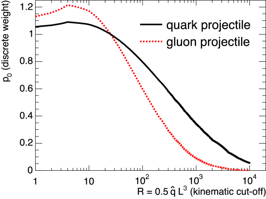
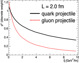
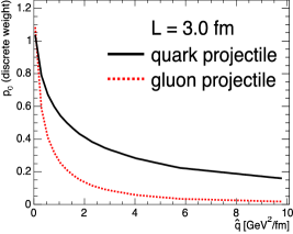
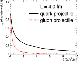
In fig. 17, top panel, we reproduce the discrete weight $p_{0}$ as a function of the kinematic constraint $R$, whereas in fig. 17, bottom panels, we show $p_{0}$ as a function of the transport coefficient $\hat{q}$ for a fixed in-medium path of $L=2\leavevmode\nobreak\ \mbox{${\rm fm}$}$ (left), $L=3\leavevmode\nobreak\ \mbox{${\rm fm}$}$ (middle) and $L=4\leavevmode\nobreak\ \mbox{${\rm fm}$}$ (right).  The probability of no medium-induced radiation decreases with increasing density of the medium. It is significantly larger for quarks than for gluons due to their lower QCD coupling. The probability to radiate at least one gluon, $1-p_{0}$, for $L=3\leavevmode\nobreak\ \mbox{${\rm fm}$}$ at $\hat{q}=1\leavevmode\nobreak\ \mbox{${\rm GeV}$}^{2}/\mbox{${\rm fm}$}$ is about $50$% for quarks and about $80$% for gluons; whereas at $\hat{q}=10\leavevmode\nobreak\ \mbox{${\rm GeV}$}^{2}/\mbox{${\rm fm}$}$ it is about $80$% quarks and almost $100$% for gluons.

Figure 18: Distribution of the continuous part of the quenching weight for quarks (left) and gluons (right) at fixed $L=3\leavevmode\nobreak\ \mbox{${\rm fm}$}$ and for different values of $\hat{q}$ .

Figure 19: Average energy loss of quarks and gluons as a function of the transport coefficient for $L=2\leavevmode\nobreak\ \mbox{${\rm fm}$}$ (left), $L=3\leavevmode\nobreak\ \mbox{${\rm fm}$}$ (middle) and $L=4\leavevmode\nobreak\ \mbox{${\rm fm}$}$ (right).

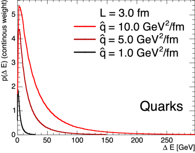
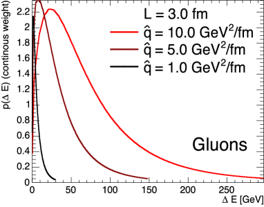
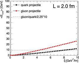
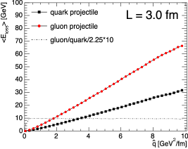
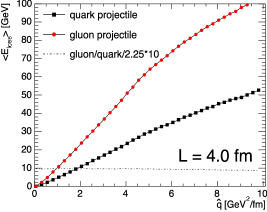
Figure 18 reports the distribution of the continuous weight $p(\Delta E)$ for quark and gluon projectiles at fixed $L=3\leavevmode\nobreak\ \mbox{${\rm fm}$}$ and for different values of $\hat{q}$. One observes that the gluon distribution is significantly broader compared to the quark distribution. This difference resulting from the different QCD coupling values of quarks and gluons is most obvious reflected in the average energy loss, $\left<\Delta E\right>$, which we plot in fig. 19 for quarks and gluons as a function of the transport coefficient for various values of the in-medium path length. The calculation takes into account both the discrete and the continuous parts of the quenching weight. As expected from eq. (11), the gluon-to-quark ratio is exactly $9/4=2.25$ and $\left<\Delta E\right>$ grows approximately linearly with the transport coefficient and, thus, with the characteristic gluon energy $\omega_{\rm c}$. We find $\left<\Delta E\right>_{\rm quarks}\approx 0.1\times\omega_{\rm c}$ for a quark and $\left<\Delta E\right>_{\rm gluons}\approx 0.25\times\omega_{\rm c}$ for a gluon projectile.

The spatially integrated energy losses in the hot medium can be translated into losses per unit path length, $\mathrm{d}E/\mathrm{d}x_{\rm quarks}\approx 0.05\,\hat{q}\,L$ and $\mathrm{d}E/\mathrm{d}x_{\rm gluons}\approx 0.125\,\hat{q}\,L$. Even for conservatively chosen values of $\hat{q}=2\leavevmode\nobreak\ \mbox{${\rm GeV}$}^{2}/\mbox{${\rm fm}$}$ and $L=3\leavevmode\nobreak\ \mbox{${\rm fm}$}$ the resulting differential losses are one order of magnitude larger than those estimated by means of the Bjorken model for the collisional energy loss. Given the $L^{2}$-dependence of the effect, the differential energy loss should be quoted per unit path length squared, leading to $\mathrm{d}^{2}E/\mathrm{d}x^{2}_{\rm quarks}\approx 0.05\,\hat{q}$. and $\mathrm{d}^{2}E/\mathrm{d}x^{2}_{\rm gluons}\approx 0.125\,\hat{q}$.

As mentioned, the evaluation of the quenching weights in the BDMPS-Z-SW model is done in the eikonal approximation (soft limit), where $\omega_{\rm c}\ll E\rightarrow\infty$ holds (cf. page 1). Since in practice calculations need to be performed at finite parton energies, we will in section 2 propose several possibilities to extrapolate to finite parton energies.

3 Hard sector at RHIC

At RHIC the available centre-of-mass energy is for the first time in the history of heavy-ion collisions high enough to allow hard scatters at the scale of $10$–$20\leavevmode\nobreak\ \mbox{${\rm GeV}$}$. Since this is too low to produce outstanding, high-energy jets to be identified on top of the heavy-ion background, the research focuses on inclusive (or leading-) particle spectra and (two-) particle correlations and their modification in nucleon–nucleon with respect to proton–proton collisions.

The suppression of high-momentum leading particles is regarded as one of the major discoveries at RHIC [160, 76]. In Au–Au collisions at various centre-of-mass energies (but mainly at $\sqrt{s_{\scriptscriptstyle{{\rm NN}}}}=200\leavevmode\nobreak\ \mbox{${\rm GeV}$}$) the two experiments with high transverse-momentum capabilities, PHENIX and STAR, but also PHOBOS and BRAHMS, have measured:

• the suppression of single-particle yields at high $p_{\mathrm{T}}$ ($\,{\buildrel>\over{{}_{\sim}}}\,4\leavevmode\nobreak\ \mbox{${\rm GeV}$}$) [161, 162, 163, 164, 165];

• the disappearance, in central collisions, of jet-like correlations in the azimuthally-opposite side (away-side) of a high-$p_{\mathrm{T}}$ leading particle [166, 167] and, quite recently, the reappearance of the particles on the away-side manifested in low-momentum hadrons [168, 169];

• the absence of these (final-state) effects in d–Au collisions at the same centre-of-mass energy [170, 171, 161, 172].

1 Leading-hadron production in factorized pQCD

Within the pQCD collinear factorization framework [84], the inclusive cross section at LO for the production of an high-$p_{\mathrm{T}}$ hadron at central rapidity in the nuclear reaction of $\rm{A}+\rm{B}\rightarrow\rm{h}+\rm{X}$ can be expressed by [173]

$$\left.\frac{\mathrm{d}^{3}\sigma_{{\rm AB}\rightarrow{\rm hX}}}{\mathrm{d}^{2}p_{\mathrm{T}}\,\mathrm{d}y}\,\right|_{y=0} = K_{\rm NLO}\,\sum_{abc}\,\int\mathrm{d}\vec{r}\,\mathrm{d}x_{a}\,\mathrm{d}x_{b}\,\mathrm{d}z_{c}$$ (15)

$$\times F_{a/\rm A}(x_{a},Q^{2},\vec{r})\,F_{b/\rm B}(x_{b},Q^{2},\,\vec{b}-\vec{r})$$

$$\times\left.\frac{\mathrm{d}^{3}\hat{s}_{ab\rightarrow c}}{\mathrm{d}^{3}p_{{\rm T},c}\,\mathrm{d}y_{c}}\,(x_{a},x_{b},Q^{2})\right|_{y_{c}=0}\;\frac{D^{\rm mod}_{{\rm h}/c}(z_{c},Q_{\rm f}^{2})}{z_{c}^{2}}\;.$$

It gives the differential cross section as a convolution of generalized PDFs $F_{a/\rm A}$ for the interacting partons with generalized FFs $D^{\rm mod}_{{\rm h}/c}$ for the leading scattered parton into the final hadron and the parton–parton differential cross sections for the contributing, elementary sub-processes.  In this context $z_{c}=p_{\mathrm{T}}/p_{{\rm T},c}$ is the momentum fraction of the hard parton, which is carried by the produced hadron. $K_{\rm NLO}$ is a phenomenological factor that is introduced to account for NLO corrections. Like the hard cross section it is $\sqrt{s}$ and scale dependent. Usually it takes values $\simeq 1-4$ [73, 174].  The various fragmentation, factorization and renormalization scales are fixed to the same value, $Q=\alpha\,Q_{\rm f}=\kappa\,p_{\mathrm{T}}$, where $1\leq\alpha\leq 3$ and $0.5\leq\kappa\leq 2$.

Equation (15) is applicable for hadron–hadron, hadron–nucleus and nucleus–nucleus interactions, and includes initial and final state effects. The generalized PDFs

$$F_{a/\rm A}(x_{a},Q^{2},\vec{b})=T_{\rm A}(\vec{b})\,\int\mathrm{d}^{2}k_{{\rm T}_{a}}\,g_{\rm A}(\vec{k}_{{\rm T}_{a}},Q^{2},\vec{b})\,f_{a/\rm A}(x_{a},Q^{2})$$ (16)

include the nuclear thickness function $T_{\rm A}$ [176]  and $\int\mathrm{d}^{2}k_{\rm T}\,g_{\rm A}$ describing intrinsic-$k_{\rm T}$ (or $k_{\rm T}$-smearing) [177] and $k_{\rm T}$-broadening for nuclei [178], as well as the nuclear modification of the PDF $f_{a/\rm A}$ (see section 3 on page 3).  The introduction of $k_{\rm T}$ is motivated by the pQCD initial state radiation to correct the computation up to transverse momenta of $p_{\mathrm{T}}\leq 4\leavevmode\nobreak\ \mbox{${\rm GeV}$}$. It is typically approximated by a Gaussian

$$g_{\rm A}(k_{\rm T})=\frac{e^{-k_{\rm T}^{2}/\langle{k}_{\rm T}^{2}\rangle}}{\pi\langle{k}_{\rm T}^{2}\rangle}\;,$$ (17)

where the width $\langle{k}_{\rm T}^{2}\rangle$ enters as a phenomenological parameter and is typically set to a value of the order of $1\leavevmode\nobreak\ \mbox{${\rm GeV}$}^{2}$. 

The generalized FFs

$$D^{\rm mod}_{{\rm h}/c}(z_{c},Q_{f}^{2})=\int\mathrm{d}\epsilon\,P(\epsilon)\,\frac{1}{1-\epsilon}\,D_{{\rm h}/c}(\frac{z_{c}}{1-\epsilon},Q_{f}^{2})$$

include the non-perturbative mechanism $D_{{\rm h}/c}$ of how the parton turns into the leading hadron (see section 5). The quenching probability, $P(\epsilon)$, denotes the possible in-medium modification in the final state [179]. Prior to hadronization the parent parton of the hadron loses an energy fraction $\epsilon=\Delta E_{c}/E_{c}$ with probability $P(\epsilon)$. Therefore, the leading hadron is a fragment of a parton with lower energy $(1-\epsilon)\,E_{z}$ and accordingly must carry a larger fraction of the parton energy $z_{c}/(1-\epsilon)$. In general, the quenching probability $P(\epsilon)$ —given by a model of parton energy loss in dense deconfined matter (see section 2)— is a function of the medium properties, the parton energy and type and the collision geometry. If no final state quenching is considered (i.e. for a nucleon) it reduces to $P(\epsilon)=\delta(\epsilon)$.

Figure 20 shows the application of eq. (15) for the production of neutral pions in pp and Au–Au collisions measured by PHENIX [170, 164]. Whereas the binary scaled pp and peripheral Au–Au data points are consistent and, both, described by NLO pQCD [175], the central yields cannot be calculated by the standard pQCD formalism (i.e. eq. (15) without modified fragmentation functions). It is precisely the breakdown of the expected incoherent parton-scattering assumption for high-$p_{\mathrm{T}}$ production in non-peripheral Au–Au collisions at RHIC energies, which recently has created much excitement. It is now attributed to strong final state effects as we outline in the next section.

(a) Peripheral $\pi_{0}$ yields ($80$–$92$%)

(b) Central $\pi_{0}$ yields ($0$–$10$%)

Figure 20: Invariant $\pi^{0}$ yields measured by PHENIX in peripheral 20(a) and in central 20(b) Au–Au collisions [164] compared to the binary scaled pp cross section [180] and to a standard NLO pQCD calculation [181]. The overall normalization uncertainties in the scaled pp yield is of the order of the symbol sizes. The figures are adapted from [182].

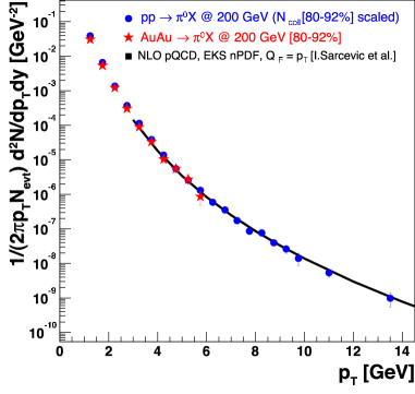
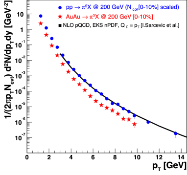
2 Leading-particle suppression as strong final state effect

The effect of the medium on the production of a hard probe is typically quantified via the ratio of the shown spectra, the nuclear modification factor,

$$R_{\rm AB}(p_{\mathrm{T}},\eta;\,b)=\frac{1}{\left<N_{\rm coll}(b)\right>}\times\frac{\mathrm{d}^{2}N^{\rm hard}_{\rm AB}/\mathrm{d}p_{\mathrm{T}}\,\mathrm{d}\eta}{\mathrm{d}^{2}N^{\rm hard}_{\rm pp}/\mathrm{d}p_{\mathrm{T}}\,\mathrm{d}\eta}\;,$$ (18)

which measures the deviation of the nucleus–nucleus from the superposition of independent nucleon–nucleon collisions. In absence of strong nuclear initial state effects it should be unity, if binary collision scaling holds according to

$$\mathrm{d}^{2}N^{\rm hard}_{\rm AB}/\mathrm{d}p_{\mathrm{T}}\,\mathrm{d}\eta=\left<N_{\rm coll}(b)\right>\times\mathrm{d}^{2}N^{\rm hard}_{\rm pp}/\mathrm{d}p_{\mathrm{T}}\,\mathrm{d}\eta\;.$$ (19)

However, in accordance with fig. 20(b), at RHIC in Au–Au collisions at $\sqrt{s_{\scriptscriptstyle{{\rm NN}}}}=200\leavevmode\nobreak\ \mbox{${\rm GeV}$}$ strong suppression effects are observed [161, 162, 163, 164, 165], visible in fig. 21, where we reproduce $R_{\rm AA}$ as a function of $p_{\mathrm{T}}$ for charged hadron and neutral pions measured at mid-pseudo-rapidity in central events by STAR and PHENIX. The magnitude of suppression is the same for charged hadrons and neutral pions beyond $p_{\mathrm{T}}\,{\buildrel>\over{{}_{\sim}}}\,5\leavevmode\nobreak\ \mbox{${\rm GeV}$}$.  In fig. 22 we show the centrality dependence of the average $R_{\rm AA}$ as a function of $N_{\rm part}$ for the same data sets. The average suppression for $p_{\mathrm{T}}>4.5\leavevmode\nobreak\ \mbox{${\rm GeV}$}$ increases from peripheral to central events, up to about a factor of $5$ in head-on collisions. Strong suppression exists also at $\sqrt{s_{\scriptscriptstyle{{\rm NN}}}}=130\leavevmode\nobreak\ \mbox{${\rm GeV}$}$ [185, 186]. Recent measurements at $\sqrt{s_{\scriptscriptstyle{{\rm NN}}}}=62.4\leavevmode\nobreak\ \mbox{${\rm GeV}$}$ show very moderate suppression for charged hadrons at intermediate $p_{\mathrm{T}}\leq 4\leavevmode\nobreak\ \mbox{${\rm GeV}$}$ [187].  Quite recently, suppression of high-$p_{\mathrm{T}}$ particles already at the highest SPS energy has been suggested [188].

Figure 21: Nuclear modification factor $R_{\rm AA}(p_{\mathrm{T}})$ at $\eta\approx 0$ in central Au–Au collisions at $\sqrt{s_{\scriptscriptstyle{{\rm NN}}}}=200\leavevmode\nobreak\ \mbox{${\rm GeV}$}$ for charged hadrons [162, 163] and neutral pions [164]. The data are reported with statistical and $p_{\mathrm{T}}$-dependent systematic errors (bars on the data points) and $p_{\mathrm{T}}$-independent systematic errors (bars at $R_{\rm AA}=1$).

Figure 22: Average nuclear modification factor $\left<R_{\rm AA}\right>$ at $\eta\approx 0$ in the range $4.5\leq p_{\mathrm{T}}\leq 10\leavevmode\nobreak\ \mbox{${\rm GeV}$}$ as a function of collision centrality (expressed by the number of participants, $N_{\rm part}$) in central Au–Au collisions at $\sqrt{s_{\scriptscriptstyle{{\rm NN}}}}=200\leavevmode\nobreak\ \mbox{${\rm GeV}$}$ for charged hadrons [162, 163] and neutral pions [164]. The error bars are the sum of statistical and $p_{\mathrm{T}}$-dependent systematic errors and the bands centered at $R_{\rm AA}=1$ are the $p_{\mathrm{T}}$-independent normalization errors for STAR (dot-dashed) and PHENIX (dashed).

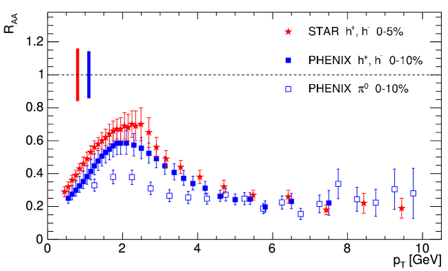
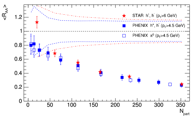
The discrepancy of the expected scaling from eq. (19) by the large factor of up to about $5$ at $\sqrt{s_{\scriptscriptstyle{{\rm NN}}}}=200\leavevmode\nobreak\ \mbox{${\rm GeV}$}$ could be addressed by the following pictures:

1. The breakdown of the leading-twist QCD collinear factorization itself. In that case the incoherence between long- and short-distance effects, on which the factorized product eq. (15) relies upon, would not hold for A–A collisions. In addition, due to strong initial effects, the nPDFs might be modified, such that $f_{a/{\rm A}}\ll A\,f_{a/{\rm p}}$ in the relevant ($x$, $Q^{2}$) range, reducing the number of effective partonic scattering centers.

2. Strong final-state effects in the deconfined medium, such as medium-induced parton energy loss (see  sectchap3:partoneloss), modify the parton fragmentation functions compared to collisions in cold matter of free space.

The first explanation is invoked by means of the CGC model [67]; the latter by models employing parton energy loss; in most cases due to medium-induced gluon radiation in the QGP, as we will outline in section 4.

(a) Control measurement (Au–Au vs. d–Au)

(b) Direct photons excess

Figure 23: 23(a) Nuclear modification factor, $R_{\rm dAu}(p_{\mathrm{T}})$ and $R_{\rm AA}(p_{\mathrm{T}})$, for neutral pions measured by PHENIX at mid-rapidity in minimum-bias d–Au [170] and central Au–Au [164] collisions, both at $\sqrt{s_{\scriptscriptstyle{{\rm NN}}}}=200\leavevmode\nobreak\ \mbox{${\rm GeV}$}$. The figure is adapted from LABEL:denterria2004. 23(b) Direct photon excess for central Au–Au collisions at $\sqrt{s_{\scriptscriptstyle{{\rm NN}}}}=200\leavevmode\nobreak\ \mbox{${\rm GeV}$}$ by PHENIX compared to NLO pQCD yields scaled by $N_{\rm coll}$. The dot-dash curve represents the expected excess, if there were no suppression of the background produced by meson decay. The figure is taken from LABEL:frantz2004.

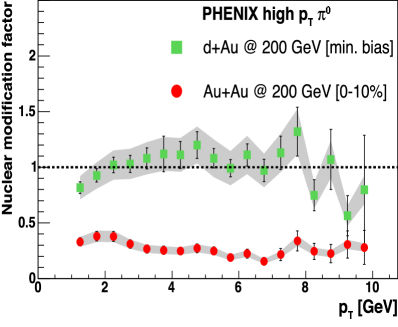
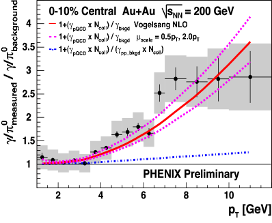
In order to disentangle between the two scenarios experimentally, it is vital to compare to measurements in d–Au collisions at the same centre-of-mass energy, where the nuclear modification factor $R_{\rm dAu}$ is determined by initial-state effects alone and no medium is expected to influence the final state. As shown in fig. 23(a) the high-$p_{\mathrm{T}}$ production of neutral pions at $\sqrt{s_{\scriptscriptstyle{{\rm NN}}}}=200\leavevmode\nobreak\ \mbox{${\rm GeV}$}$ in d–Au is due to $k_{\mathrm{T}}$-broadening (Cronin effect) even slightly enhanced ($R_{\rm dAu}\sim 1.1$) [170]. This confirms that the suppression in Au–Aufor central collisions cannot be explained by initial-state effects. Further experimental evidence supporting the suppression driven by the formation of the dense partonic matter is the measurement of direct photon excess from PHENIX [189]. Figure 23(b) shows the double-ratio of $\mathrm{d}N^{\rm total}_{\gamma}/\mathrm{d}p_{\mathrm{T}}$ over $\mathrm{d}N^{\rm decay}_{\gamma}/\mathrm{d}p_{\mathrm{T}}$ normalized by the $\pi_{0}$ spectra. It is consistent with $N_{\rm coll}$ scaling as expected for an electro-magnetic (hard) probe since it is by its nature not sensitive to final-state medium effects.

3 Disappearance and reappearance of the away-side correlations

Another prominent result from RHIC measured by STAR at $\sqrt{s_{\scriptscriptstyle{{\rm NN}}}}=200\leavevmode\nobreak\ \mbox{${\rm GeV}$}$ is the disappearance of jet-like azimuthal correlations in the opposite direction (away-side) of high-$p_{\mathrm{T}}$ particles [166, 167].

(a) Sketch of in/out-plane

(b) Associated particle correlation in azimuth

Figure 24: 24(a) Definition of in-plane and out-of-plane direction. Particle emission into the azimuthal cone of 45 degrees around the reaction plane given by the impact parameter (parallel to the $x$-axis in the sketch) and the $z$-axis is called in-plane. Emission into the vertical cone of 45 degrees is out-of-plane. Every other direction is (in-) between-plane. 24(b) Azimuthal distributions of associated particles ($2\leq p_{\mathrm{T}}\leq p_{\mathrm{T}}^{\rm trig}$) assigned to high-$p_{\mathrm{T}}$ trigger particles ($4\leq p_{\mathrm{T}}^{\rm trig}\leq 6\leavevmode\nobreak\ \mbox{${\rm GeV}$}$), emitted in-plane and out-of-plane in Au–Au collisions at $\sqrt{s_{\scriptscriptstyle{{\rm NN}}}}=200\leavevmode\nobreak\ \mbox{${\rm GeV}$}$ for $20$–$60$% centrality, compared to the pp reference at the same energy, measured by STAR [167]. The contribution of the elliptic flow ($v_{2}$) is subtracted. Further details are in the text.

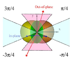
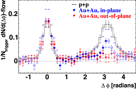
The effect is usually quantified using the correlation strength [190]

$$D_{\rm AA}=\int^{p_{\rm t,1}}_{p_{\mathrm{T}}^{\rm min}}\mathrm{d}p_{\rm t,2}\int_{\Delta\phi>\Delta\phi^{\rm min}}\mathrm{d}\Delta\phi\,\frac{\mathrm{d}^{3}\sigma_{\rm AA}^{\rm{h}_{1}\rm{h}_{2}}/\mathrm{d}p_{\rm t,1}\,\mathrm{d}p_{\rm t,2}\,\mathrm{d}\Delta\phi}{\mathrm{d}\sigma_{\rm AA}^{h_{1}}/\mathrm{d}p_{\rm t,1}}$$ (20)

for an associated particle $\rm{h}_{2}$ with transverse momentum $p_{\rm t,2}$ in the opposite azimuthal direction of a ‘trigger’ particle $\rm{h}_{1}$ with transverse momentum $p_{\rm t,1}$. The existing data allows trigger particles with $4<p_{\rm t,1}<6\leavevmode\nobreak\ \mbox{${\rm GeV}$}$ and associated particles with $p_{\rm t,2}>p_{\mathrm{T}}^{\rm min}=2\leavevmode\nobreak\ \mbox{${\rm GeV}$}$ and $p_{\rm t,2}<p_{\rm t,1}$, with $\Delta\phi\equiv|\phi_{1}-\phi_{2}|>\Delta\phi^{\rm min}=130^{\circ}$.  The correlation strength is then corrected for combinatorial background and azimuthal anisotropy of particle production in non-central collisions. The picture which emerged is that as central collisions are approached for increasing participants, the away-side correlations are gradually disappearing, until for most central collisions no correlation is observed (see fig. 32(b)).

Recently, the correlation has been measured depending on the emission direction of the trigger particle in non-central collisions [167]. Since in non-central reactions the overlap nucleus–nucleus region has an almond-like shape with shorter length in the in-plane than in the out-of-plane direction, energy loss of partons which depends on the distance traveled through the medium should differ for the two directions. The definition of the direction for particle emission into in-plane, out-of-plane and between-plane in a semi-peripheral collision is illustrated in fig. 24(a). In fig. 24(b) we show the azimuthal distribution of associated particles, defined by $2\leq p_{\mathrm{T}}\leq p_{\mathrm{T}}^{\rm trig}$, in Au–Au collisions at $20$–$60$% centrality and in pp reference data. Depending on the direction of the trigger particle (with $4\leq p_{\mathrm{T}}^{\rm trig}\leq 6\leavevmode\nobreak\ \mbox{${\rm GeV}$}$) , the associated particles are classified into different classes, in-plane or out-of-plane. The Au–Au data are corrected for collective effects, by subtracting the elliptic flow component ($v_{2}$). The near-side ($|\Delta\phi|\,{\buildrel<\over{{}_{\sim}}}\,0.5$) correlations measured in Au–Au are clearly jet-like and very similar to those in pp collisions (and to those in d–Au [171], not shown here). The back-to-back correlations ($|\Delta\phi-2\pi|\,{\buildrel<\over{{}_{\sim}}}\,0.7$) in Au–Au collisions for trigger particles emitted in-plane are suppressed compared to pp (and to d–Au [171], not shown here), and even more suppressed for the out-of-plane trigger particles.

Figure 25: Transverse-momentum distributions of near-side (a) and away-side (b) associated particles for pp, peripheral and central Au–Au collisions at $\sqrt{s_{\scriptscriptstyle{{\rm NN}}}}=200\leavevmode\nobreak\ \mbox{${\rm GeV}$}$ measured by STAR. The bands show the systematic errors for central collisions. Ratios of the Au–Au to pp distributions for the near-side (c) and the away-side (d). The figure is taken from LABEL:wang2004.

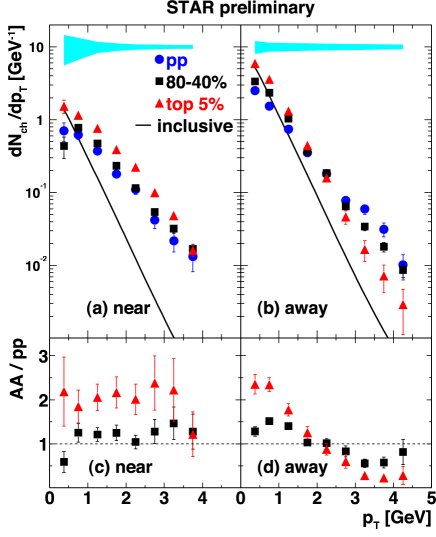
Since energy must be conserved, it is expected that particles on the away-side should be rather soft, originating from thermalized (former hard) partons. Indeed, the reappearance of the particles on the away-side recently has been confirmed in low-momentum hadrons [168]. Figure 25 shows the $p_{\mathrm{T}}$-distribution of associated particles in pp, peripheral ($40$–$80$%) and central ($0$–$5$%) Au–Au collisions at $\sqrt{s_{\scriptscriptstyle{{\rm NN}}}}=200\leavevmode\nobreak\ \mbox{${\rm GeV}$}$. While agreement is found between pp and the peripheral Au–Au data on both sides, the central Au–Au results differ from pp, most significantly for the away-side. The ratios of the Au–Au to pp distributions indicate that the leading partons are modified in the medium created in the central Au–Au collisions. The modifications lead to more associated particles on the near side, and shifts energy from high to low momentum on the away side.

In summary, the present, high-$p_{\mathrm{T}}$ observations at RHIC lead to the ‘model-independent’ conclusion that partons traversing the dense medium in the core of the collision lose the majority of their energy, and the observed jet fragments are primarily those created from partons produced near the surface and directed outwards. In the next section we will try to give a quantitative description of these experimental findings.

4 The Parton Quenching Model

The experimental observations at RHIC have been explained in terms of attenuation or quenching models, where the energetic partons produced in the initial hard scattering processes as a consequence of the interaction with the dense QCD medium ‘loose’ energy. Several works exist on the subject [178, 192, 179, 190, 193, 194, 195, 1, 196]. Most models implement the parton energy loss due to medium-induced gluon radiation (see section 2). Also hadronic interactions [197, 198] have been investigated and found to contribute to the observed depletion of the hadron spectra.

In the following we describe the PQM [1], which combines the parton energy loss in the BDMPS-Z-SW framework with a realistic collision geometry given by the Glauber model. The leading-particle suppression in A–A collisions is obtained evaluating eq. (15) in a Monte Carlo approach. The transverse momentum distributions for charged hadrons are generated by means of the following steps:

1. Generation of a quark or gluon with $p_{\mathrm{T}}>3\leavevmode\nobreak\ \mbox{${\rm GeV}$}$, using PYTHIA [119, 120, 121] in pp mode with the CTEQ 4L PDF [58];

2. determination of the parameters, $\omega_{\rm c}$ and $R$, eq. (8) and eq. (9), for the calculation of the quenching weights and the energy-loss probability distribution $P(\Delta E)$ eq. (14);

3. Monte Carlo sampling of the energy loss $\Delta E$ according to $P(\Delta E)$ to assign the quenched parton transverse momentum, $p_{\mathrm{T}}^{\prime}=p_{\mathrm{T}}-\Delta E$;

4. hadronization of the quenched parton using the KKP fragmentation functions [126].

Steps 2 and 3 will be explained in more detail in the following paragraphs. The quenched and unquenched $p_{\mathrm{T}}$-distributions are obtained including or excluding the third step. The nuclear modification factor $R_{\rm AA}(p_{\mathrm{T}})$, eq. (18), is simply given by their ratio.

Figure 26: Comparison between the charged hadron yield in pp collisions measured and parameterized by PHENIX [180] and the calculation by PQM.

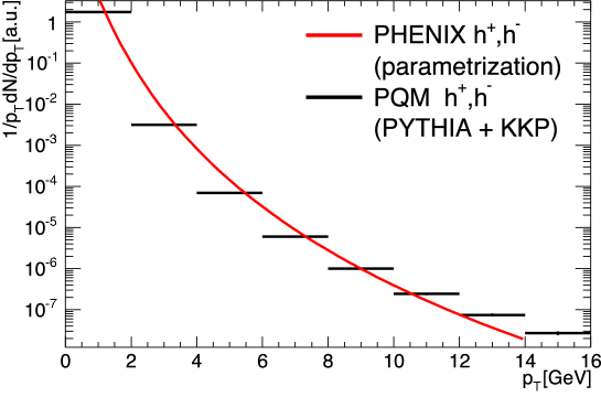
In fig. 26 we show that the hadron $p_{\mathrm{T}}$-distribution at $\sqrt{s}=200\leavevmode\nobreak\ \mbox{${\rm GeV}$}$ agrees in shape with that measured for neutral pions in pp collisions by PHENIX [180]. The $\mathrm{\pi^{0}}$ data has been parameterized according to

$$\frac{1}{p_{\mathrm{T}}}\,\frac{\mathrm{d}^{2}N}{\mathrm{d}p_{\mathrm{T}}\mathrm{d}\eta}=\mathrm{const}\,(1+\frac{p_{0}}{p_{\mathrm{T}}})^{-n}\,r(p_{\mathrm{T}})\;,$$

where $p_{0}=1.22\leavevmode\nobreak\ \mbox{${\rm GeV}$}$ and $n=10$. For the correction from neutral pions to charged hadrons we use a constant value of $r=1.6$.

1 Parton-by-parton approach

The probability distribution $P(\Delta E)$, eq. (14), depends on the kinematical cutoff $R$ and on the characteristic gluon frequency $\omega_{\rm c}$. Due to the fact that $\hat{q}$ and $L$ are intuitively and physically more meaningful parameters, in most applications of the quenching weights [155, 199, 196] the ($R$, $\omega_{\rm c}$)-dependence of the quenching weights has been turned into a ($\hat{q}$, $L$)-dependence, via eq. (8) and eq. (9).

The standard approach has been to fix a value for the transport coefficient, the same for all produced partons, and either to use a constant (effective) in-medium length [155] or to calculate a different length for each parton according to a description of the collision geometry [199, 196]. However, that approach is not optimal, because there is no unique and exact definition of the in-medium path length when a realistic nuclear density profile is considered and the medium density is not constant over the whole nucleus–nucleus overlap region, but rather decreasing from the inner to the outer layers.

In order to overcome these limitations, in PQM we introduce an alternative approach. Namely, we determine the two parameters $\omega_{\rm c}$ and $R$ on a parton-by-parton basis: For a given centrality, the (transverse) density profile of the matter is computed and for each produced parton in the collision its path (azimuthal direction and length) through the matter determined. We, thus, need to replace the fixed values of $\hat{q}$ and $L$ with their respective distributions as ‘seen’ by the partons on the way out. Starting from eq. (8) and using eq. (13) (for $\xi_{0}=0)$ with a space-point dependent transport coefficient $\hat{q}(\xi)$ and a path-averaged $\left<\hat{q}\right>$, we define the effective quantity

$$\omega_{\rm c}\left|{}_{\rm effective}\right.\equiv\frac{1}{2}\left<\hat{q}\right>\,L^{2}=\int_{0}^{\infty}\xi\,\hat{q}(\xi)\,\mathrm{d}\xi\;,$$ (21)

which on the r.h.s. does not explicitly depend on $L$ anymore. Similarly, we define

$$\left<\hat{q}\right>L\left|{}_{\rm effective}\right.\equiv\int_{0}^{\infty}\hat{q}(\xi)\,\mathrm{d}\xi$$ (22)

and

$$R\left|{}_{\rm effective}\right.\equiv\frac{2\,\left(\omega_{\rm c}\left|{}_{\rm effective}\right)^{2}\right.}{\left<\hat{q}\right>L\left|{}_{\rm effective}\right.}\;.$$ (23)

For a step-function density distribution $\hat{q}(\xi)=\hat{q}_{0}\,\theta(L-\xi)$, eq. (21) and eq. (23) coincide with eq. (8) and eq. (9).

Using the definitions given by eq. (21) and eq. (23) we incorporate the geometry of the collision via the local, space-point dependent, transport coefficient $\hat{q}(\xi)$. The geometry is defined in the ($x$, $y$) plane transverse to the beam direction $z$, in which the centers of two nuclei A and B colliding with an impact parameter $b$ have the coordinates ($-b/2$, $0$) and ($b/2$, $0$), respectively. We use the Glauber model (see section 7.A) to describe the geometry of the collision assuming the distribution of parton production points in the transverse plane and the transverse density of the medium both to be proportional to the $b$-dependent product $T_{\rm A}\,T_{\rm B}(x,y;\,b)\equiv T_{\rm A}(x,y)\times T_{\rm B}(x,y)$; given by the thickness functions of the two nuclei. The nuclear thickness function is defined as the $z$-integrated Wood-Saxon nuclear density profile: $T_{\rm i}(x,y)\equiv\int\mathrm{d}z\,\rho_{\rm i}^{\rm WS}(x,y,z)$. The parameters of the Wood-Saxon profile for different nuclei are tabulated from data [200]. Note that $T_{\rm A}\,T_{\rm B}(x,y;\,b)$ estimates the transverse density of binary NN collisions, $\rho_{\rm coll}(x,y;b)$, modulo the inelastic NN cross section.

Since we only consider partons produced at very central rapidities, we assume that they propagate in the transverse plane ($E\approx p\approx p_{\mathrm{T}}$). For a parton with production point ($x_{0}$, $y_{0}$) and azimuthal propagation direction ($\cos\phi_{0}$, $\sin\phi_{0}$) ($\phi_{0}$ is sampled uniformly), we define the local transport coefficient along the path of the parton inside the overlap region of the nuclei as

$$\hat{q}(\xi;b)=k\times T_{\rm A}\,T_{\rm B}(x_{0}+\xi\cos\phi_{0},y_{0}+\xi\sin\phi_{0};\,b)\;.$$ (24)

The parameter $k$ (in ${\rm fm}$) is used to set the scale of the transport coefficient (in $\mbox{${\rm GeV}$}^{2}/\mbox{${\rm fm}$}$). It is the only parameter in PQM. The idea is to keep $k$ fixed, once it is determined by a fit to the data. For every parton (or every pair of partons in opposite directions) we compute the two integrals $I_{0}$ and $I_{1}$ given by eq. (21) and eq. (22)

$$I_{n}\equiv\int_{0}^{\infty}\xi^{n}\,\hat{q}(\xi;b)\,\mathrm{d}\xi\hskip 28.45274ptn=0,\,1\;,$$

which determine the energy-loss probability distribution $P(\Delta E)$ according to

$$\omega_{\rm c}\left|{}_{\rm effective}\right.=I_{1}\hskip 14.22636pt{\rm and}\hskip 14.22636ptR\left|{}_{\rm effective}\right.=2\,I_{1}^{2}/I_{0}\;.$$ (25)

And for the corresponding effective path length and transport coefficient we get

$$L\left|{}_{\rm effective}\right.=2\,I_{1}/I_{0}\hskip 14.22636pt{\rm and}\hskip 14.22636pt\hat{q}\left|{}_{\rm effective}\right.=I_{0}^{2}/(2\,I_{1})\;.$$ (26)

We point out that the resulting definition of $L$  is, as necessary, independent of $k$. Furthermore, it is the same used in LABEL:dainese2003. Note that the effective $\hat{q}$ is proportional to $k$.

Figure 27: Distributions of parton production points in the transverse plane (upper row) and effective (eq. (26)) in-medium path length (lower row) in central, semi-central and peripheral Au–Au collisions. The quantity $\left<L\right>$ is the average of the path-length distribution.

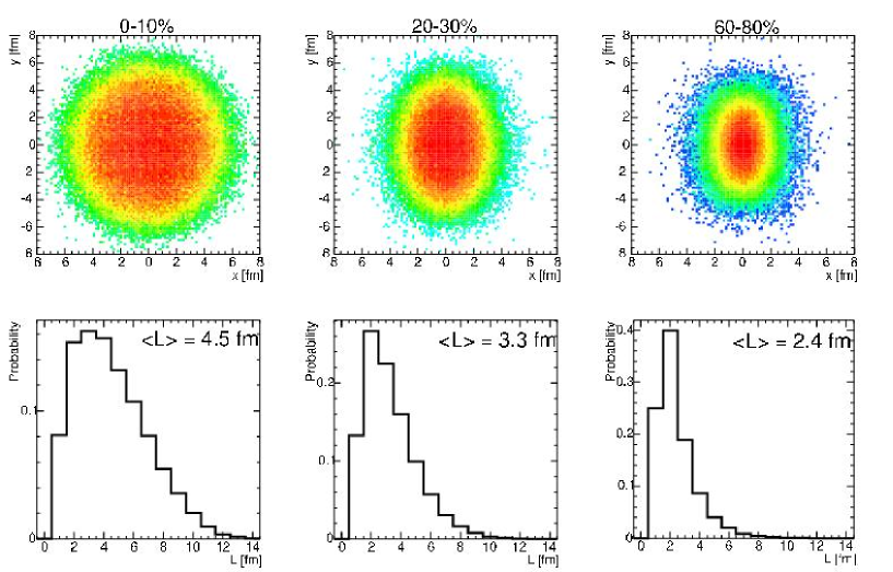
The parton-by-parton approach allows a natural extension from central to peripheral nucleus–nucleus collisions. After the only free parameter, $k$, is determined to describe the measured nuclear modification factor in central collisions at $\sqrt{s_{\scriptscriptstyle{{\rm NN}}}}=200\leavevmode\nobreak\ \mbox{${\rm GeV}$}$, the results for other centrality classes simply depend on the impact parameter dependence of the product $T_{\rm A}\,T_{\rm B}(x,y;\,b)$. By means of the Glauber model, we translate the experimental definition of the centrality classes in terms of fractions of the geometrical cross section to a range in $b$. Within such range, we sample, for every parton (or every parton pair) a value of $b$ according to the $b$-dependence of the average number of binary collisions, $\mathrm{d}\left<N_{\rm AB}^{\rm coll}\right>/\mathrm{d}b$. In fig. 27 we report the distributions of the parton production points ($x_{0}$, $y_{0}$) in the transverse plane and of the effective in-medium path lengths, eq. (26), in central ($0$–$10$%), semi-central ($20$–$30$%) and peripheral (60–80%) Au–Au collisions obtained with PQM. The average length decreases from $\left<L\right>=4.4\leavevmode\nobreak\ \mbox{${\rm fm}$}$ for most central, to $3.3\leavevmode\nobreak\ \mbox{${\rm fm}$}$ for semi-central, down to $2.4\leavevmode\nobreak\ \mbox{${\rm fm}$}$ for peripheral collisions.

Figure 28: Distributions of effective $\hat{q}$ (eq. (26)), for different centralities. The $k$ parameter, setting the scale, is fixed to the value $k=5\cdot 10^{6}\leavevmode\nobreak\ \mbox{${\rm fm}$}$ that allows to describe $R_{\rm AA}$ for the most central Au–Au collisions at $\sqrt{s_{\scriptscriptstyle{{\rm NN}}}}=200\leavevmode\nobreak\ \mbox{${\rm GeV}$}$.

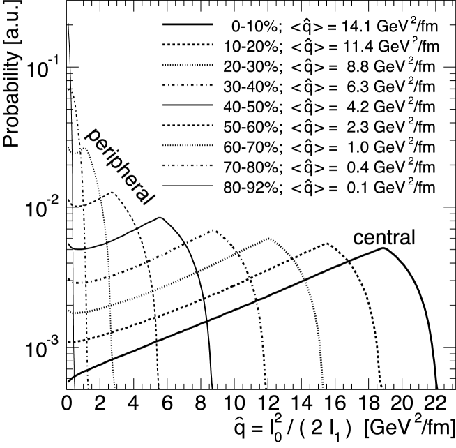
In fig. 28 we show the distributions of effective $\hat{q}$, eq. (26), for different centralities. The scale $k$ is fixed to the value $k=5\cdot 10^{6}\leavevmode\nobreak\ \mbox{${\rm fm}$}$ that allows to describe $R_{\rm AA}$ for the most central Au–Au collisions at $\sqrt{s_{\scriptscriptstyle{{\rm NN}}}}=200\leavevmode\nobreak\ \mbox{${\rm GeV}$}$ (see below). The $\hat{q}$ variation within a given centrality class reflects the different parton production points and, hence, the different medium densities encountered by the partons on their way out of the interaction region. The rightmost (highest) value refers to partons originating from the border of almond region and traversing through the complete interior of the dense collision center.

2 Finite energy constraints

For the calculation of the energy loss in PQM we use the quenching weights in the BDMPS-Z-SW framework, introduced in section 2. According to the $P(\Delta E)$ distribution, obtained by the parameters $\omega_{\rm c}$ and $R$ as explained in the previous section, we sample the energy loss $\Delta E$, to get the reduced parton transverse momentum, $p_{\mathrm{T}}^{\prime}=p_{\mathrm{T}}-\Delta E$.

The quenching weights are calculated in the eikonal approximation, in which the energy of the primary parton is infinite ($E=p_{\mathrm{T}}=\infty$). Therefore, when the realistic case of finite-energy partons is considered, a significant part of the energy-loss probability distribution $P(\Delta E)$ lies above the parton energy $E$, in particular for large values of $\omega_{\rm c}$ and $R$, or equivalently, of $\hat{q}$ and $L$. Since for a parton with energy $E$ the energy loss must be constrained to $\Delta E\leq E$, we define the constrained weights according to the following two prescriptions:

• Reweighted: Truncate $P(\Delta E)$ at $\Delta E=E$, and renormalize it to unity

  $$P^{\rm rw}(\Delta E,\,E)=\frac{P(\Delta E)\,\Theta(E-\Delta E)}{\int_{0}^{E}\,\mathrm{d}\epsilon\,P(\epsilon)}\;.$$ (27)

  The Monte Carlo implementation of this approach is: sample $\Delta E$ from the original $P(\Delta E)$; if $\Delta E>E$, sample another $\Delta E$; iterate until a $\Delta E\leq E$ is sampled.

• Non-reweighted: Truncate $P(\Delta E)$ at $\Delta E=E$ and add $\delta(E-\Delta E)\int_{E}^{\infty}\mathrm{d}\epsilon\,P(\epsilon)$

  $$P^{\rm non-rw}(\Delta E,\,E)=P(\Delta E)\,\Theta(E-\Delta E)+\delta(E-\Delta E)\int_{E}^{\infty}\mathrm{d}\epsilon\,P(\epsilon)\;.$$ (28)

  The integral of $P$ is, in this way, maintained equal to one. The corresponding Monte Carlo implementation reads: sample an energy loss $\Delta E$ from the original $P(\Delta E)$; set $\Delta E=E$ if $\Delta E\geq E$.

Like the unconstrained weights the constrained quenching probabilities depend also on the kinematical parameters, $\omega_{\rm c}$ and $R$. Note, as necessary, in the eikonal limit $E\rightarrow\infty$ the constrained weights approach the unconstrained weights

$$\lim_{E\rightarrow\infty}P^{\rm rw}(\Delta E,\,E)=\lim_{E\rightarrow\infty}P^{\rm non-rw}(\Delta E,\,E)=P(\Delta E)\;.$$

Whereas, in the limit $E\rightarrow 0$ the constrained weights reduce to

$$\lim_{E\rightarrow\,0}P^{\rm rw}(\Delta E,\,E)=\lim_{E\rightarrow\,0}P^{\rm non-rw}(\Delta E,\,E)=\delta(\Delta E)\;.$$

(a) Non-reweighted energy-loss distribution

(b) Reweighted energy-loss distribution

Figure 29: Energy-loss distribution $P^{\rm non-rw}(\Delta E,\,E)$ 29(a) and $P^{\rm rw}(\Delta E,\,E)$ 29(b) for $E=100\leavevmode\nobreak\ \mbox{${\rm GeV}$}$ partons. The calculation uses fixed values of $\hat{q}=1\leavevmode\nobreak\ \mbox{${\rm GeV}$}^{2}/\mbox{${\rm fm}$}$ and $L=6\leavevmode\nobreak\ \mbox{${\rm fm}$}$, resulting in $\omega_{\rm c}=91\leavevmode\nobreak\ \mbox{${\rm GeV}$}$ and $R=2782$.

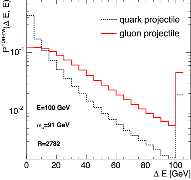
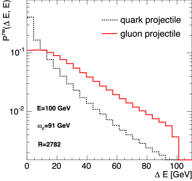
Figure 29 shows the energy-loss distribution of quarks and gluons with primary energy of $E=100\leavevmode\nobreak\ \mbox{${\rm GeV}$}$ for the non-reweighted and reweighted case. The calculation is done using fixed values of $\hat{q}=1\leavevmode\nobreak\ \mbox{${\rm GeV}$}^{2}/\mbox{${\rm fm}$}$ and $L=6\leavevmode\nobreak\ \mbox{${\rm fm}$}$, which results in $\omega_{\rm c}=91\leavevmode\nobreak\ \mbox{${\rm GeV}$}$ and $R=2782$. The average loss in the non-reweighted case is $14\leavevmode\nobreak\ \mbox{${\rm GeV}$}$ for quarks and $30\leavevmode\nobreak\ \mbox{${\rm GeV}$}$ for gluons; in the reweighted case it is $12\leavevmode\nobreak\ \mbox{${\rm GeV}$}$ for quarks and $26\leavevmode\nobreak\ \mbox{${\rm GeV}$}$for gluons. In the non-reweighted case the accounted energy loss is generally larger, since the medium with a probability $\int_{E}^{\infty}\mathrm{d}\epsilon\,P(\epsilon)$ may fully absorb the primary partons.

It has been argued [155, 196] that the difference in the values of the observables for the two different constraints illustrates the theoretical uncertainties of the BDMPS-Z-SW framework evaluated at finite parton energies. Therefore, along the lines of what has been done in Refs. [196, 1] we display the PQM results as a band delimited by the reweighted case (smaller quenching) and the non-reweighted case (larger quenching).

3 PQM results at RHIC

We will present the PQM results on the nuclear modification factor; further calculations concerning azimuthally-differential observables are reported in LABEL:dainese2004.

Before moving to the parton-by-parton approach of PQM outlined in the previous sections, it is very instructive to perform the calculation of $R_{\rm AA}(p_{\mathrm{T}})$ in Au–Au collisions at $\sqrt{s_{\scriptscriptstyle{{\rm NN}}}}=200\leavevmode\nobreak\ \mbox{${\rm GeV}$}$ defined by eq. (18) using a constant transport coefficient and the Glauber-based path-length distributions. The model results as well as the data ranging in centrality from $0$–$10$% to $80$–$92$% are shown in fig. 30. The data on charged hadrons from STAR [162] and PHENIX [164] and neutral pions from PHENIX [163] are reported with combined statistical and $p_{\mathrm{T}}$-dependent systematic errors given by the bars on the data points and $p_{\mathrm{T}}$-independent normalization errors given by the bars centered at $R_{\rm AA}=1$. We fix the transport coefficient to $\hat{q}\simeq 15\leavevmode\nobreak\ \mbox{${\rm GeV}$}^{2}/\mbox{${\rm fm}$}$ such that the data for the most central collisions are within the model band delimited by the reweighted and non-reweighted cases. For the most central case, using the constant transport coefficient of $15\leavevmode\nobreak\ \mbox{${\rm GeV}$}^{2}/\mbox{${\rm fm}$}$ and the realistic length distribution, the measured hadron suppression can be fairly well described for $p_{\mathrm{T}}\,{\buildrel>\over{{}_{\sim}}}\,5\leavevmode\nobreak\ \mbox{${\rm GeV}$}$. At lower $p_{\mathrm{T}}$ we do not apply the model, since initial-state effects and in-medium hadronization, that we do not include, might play an important role. However, as clearly observed in fig. 30, using the same constant value for $\hat{q}$ with corresponding length distribution for the different centrality classes fails to reproduce the data for semi-central and peripheral collisions. We note that between the non-reweighted and reweighted constraint there is a difference of about a factor 2 in the magnitude of $R_{\rm AA}$. In addition, there is a change in the slope, which is slightly positive in the non-reweighted and slightly negative in reweighted case.

Figure 30: $R_{\rm AA}(p_{\mathrm{T}})$ for fixed $\hat{q}=15\leavevmode\nobreak\ \mbox{${\rm GeV}$}^{2}/\mbox{${\rm fm}$}$ See caption of fig. 31.

Figure 31: $R_{\rm AA}(p_{\mathrm{T}})$ for fixed $k=5\cdot 10^{6}\leavevmode\nobreak\ \mbox{${\rm fm}$}$ in the PQM parton-by-parton approach at mid-pseudo-rapidity for different centralities in Au–Au collisions at $\sqrt{s_{\scriptscriptstyle{{\rm NN}}}}=200\leavevmode\nobreak\ \mbox{${\rm GeV}$}$. The measured points are for charged hadrons (stars, closed squares) [162, 163] and neutral pions (open squares) [164]. The data are reported with statistical and $p_{\mathrm{T}}$-dependent systematic errors (bars on the data points) and $p_{\mathrm{T}}$-independent systematic errors (bars at $R_{\rm AA}=1$).

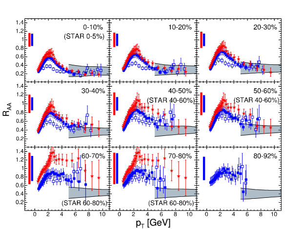
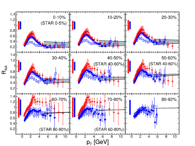
In order to address the centrality dependence of the high-$p_{\mathrm{T}}$ suppression, we move to the parton-by-parton approach by PQM. For the most central collisions, the result obtained with the scale parameter $k=5\cdot 10^{6}\leavevmode\nobreak\ \mbox{${\rm fm}$}$ matches the data. From now on, we keep the same value of $k$ and merely vary the centrality by using dependence of the local transport coefficient via eq. (24) as outlined above. The PQM parton-by-parton calculation is shown in fig. 31. The results nicely follow the increase of the measured $R_{\rm AA}$ with decreasing centrality. The theoretical uncertainty band for the most central cases is very similar to that reported in fig. 30. It is narrower for semi-central and peripheral collisions. As we will argue below the reason is that due to smaller size and density of the medium the probability to have $\Delta E>E$ in the quenching weights becomes less likely, and, therefore the differences introduced by the two constraints reduces. Note that the value of $k=5\cdot 10^{6}\leavevmode\nobreak\ \mbox{${\rm fm}$}$ corresponds to $\left<\hat{q}\right>\simeq 14\leavevmode\nobreak\ \mbox{${\rm GeV}$}^{2}/\mbox{${\rm fm}$}$ in most central collisions (see fig. 28). Numerically, our value of $\left<\hat{q}\right>\simeq 14\leavevmode\nobreak\ \mbox{${\rm GeV}$}^{2}/\mbox{${\rm fm}$}$ is smaller than $\hat{q}\simeq 10\leavevmode\nobreak\ \mbox{${\rm GeV}$}^{2}/\mbox{${\rm fm}$}$ found in LABEL:eskola2004 for central collisions. However, this is not an inconsistency. The value of $\alpha_{\rm S}$ used in the calculation of the quenching weights is $\alpha_{\rm S}=1/3$ here and $\alpha_{\rm S}=1/2$ there. Since the scale of the energy loss is set by the product $\alpha_{\rm S}\,\left<\hat{q}\right>$ (see eq. (11)), the product is about the same for both calculations. Our results for the nuclear modification factor at RHIC are summarized in fig. 32(a), where we show the average $R_{\rm AA}$ in the range $4.5<p_{\mathrm{T}}<10\leavevmode\nobreak\ \mbox{${\rm GeV}$}$ compared to data [162, 163, 164] plotted as a function of the number of participant nucleons, $N_{\rm part}$, obtained from the Glauber model.

(a) Nuclear modification factor

(b) Suppression factor

Figure 32: PQM for $k=5\cdot 10^{6}\leavevmode\nobreak\ \mbox{${\rm fm}$}$ compared to RHIC data as a function of the number of participants, $N_{\rm part}$. 32(a) Average $R_{\rm AA}$ in the range $4.5\leq p_{\mathrm{T}}\leq 10\leavevmode\nobreak\ \mbox{${\rm GeV}$}$. Data are from Refs. [162, 163, 164]. The error bars are combined statistical and $p_{\mathrm{T}}$-dependent systematic errors and the bands centered at $R_{\rm AA}=1$ are the $p_{\mathrm{T}}$-independent normalization errors for PHENIX (dashed) and STAR (dot-dashed). 32(b) $I_{\rm AA}$ for the away-side jet. Data are from STAR [166]. The statistical (bars) and systematic (ticks) errors are shown.

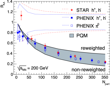
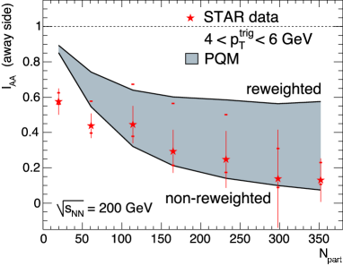
By generating pairs of back-to-back partons, we can study the centrality dependence of the disappearance of the away-side jet within the PQM framework. Using the correlation strength, eq. (20), in NN relative to pp collisions one conveniently defines the suppression factor

$$I_{\rm AA}=\frac{D_{\rm AA}}{D_{\rm pp}}\;.$$ (29)

For each parton we calculate $\omega_{\rm c}$ and $R$ and apply energy loss and fragmentation as outlined above. We count as trigger particle every hadron $\rm{h}_{1}$ with $4<p_{\rm t,1}<6\leavevmode\nobreak\ \mbox{${\rm GeV}$}$ and as associated away-side particle the other hadron $\rm{h}_{2}$ of the pair, if its transverse momentum is in the range $2\leavevmode\nobreak\ \mbox{${\rm GeV}$}<p_{\rm t,2}<p_{\rm t,1}$.

$$I_{\rm AA}=\left(\frac{N^{\rm associated}}{N^{\rm trigger}}\right)_{\rm with\leavevmode\nobreak\ energy\leavevmode\nobreak\ loss}\bigg{/}\left(\frac{N^{\rm associated}}{N^{\rm trigger}}\right)_{\rm w/o\leavevmode\nobreak\ energy\leavevmode\nobreak\ loss}\,.$$ (30)

Figure 32(b) shows the PQM result for $I_{\rm AA}$ versus $N_{\rm part}$, compared to STAR measurements [166] in Au–Au collisions at $\sqrt{s_{\scriptscriptstyle{{\rm NN}}}}=200\leavevmode\nobreak\ \mbox{${\rm GeV}$}$ with statistical (bars) and systematic (ticks) errors. The magnitude and centrality dependence of the suppression are described without changing the scale parameter value we extracted from $R_{\rm AA}$ in central collisions.

4 Extrapolation to the LHC energy

Within the PQM model the choice of the scale parameter $k$ and, hence, of the (average) transport coefficient is the main unknown for the extrapolation from RHIC to LHC energies. It is expected that the transport coefficient grows linearly with the initial (gluon) number-density of the medium [154, 156], $\hat{q}\propto n^{\rm gluons}\propto\epsilon^{3/4}$. For collisions of two nuclei with mass number $A$ at energy $\sqrt{s_{\scriptscriptstyle{{\rm NN}}}}$ the initial gluon density in the EKRT saturation model [14] is estimated to scale as

$$n^{\rm gluons}\propto{\rm A}^{0.383}\,\left(\sqrt{s_{\scriptscriptstyle{{\rm NN}}}}\right)^{0.574}.$$ (31)

Thus, we get for central Pb–Pb collisions at LHC energies

$$n^{\rm gluons}_{\rm Pb-Pb,\,5.5\,TeV}\simeq 7\times n^{\rm gluons}_{\rm Au-Au,\,200\,GeV}\;,$$

i.e. $\left<\hat{q}\right>^{\rm LHC}\simeq 100\leavevmode\nobreak\ \mbox{${\rm GeV}$}^{2}/\mbox{${\rm fm}$}$. According to eq. (24) and eq. (26) the scaling can be carried over to the $k$ parameter, $k^{\rm LHC}\simeq 3.5\cdot 10^{7}\leavevmode\nobreak\ \mbox{${\rm fm}$}$. To compute the expected nuclear modification factor in Pb–Pb collisions at the LHC we use PQM as before, but generate the parton momenta with PYTHIA at $\sqrt{s}=5.5\leavevmode\nobreak\ \mbox{${\rm TeV}$}$.

Figure 33: PQM predictions of $R_{\rm AA}(p_{\mathrm{T}})$ in Pb–Pb collisions at $\sqrt{s_{\scriptscriptstyle{{\rm NN}}}}=5.5\leavevmode\nobreak\ \mbox{${\rm TeV}$}$ for different centrality classes, as well as the Au–Au results at $\sqrt{s_{\scriptscriptstyle{{\rm NN}}}}=200\leavevmode\nobreak\ \mbox{${\rm GeV}$}$. The prediction for by Vitev and Gyulassy is taken from LABEL:vitev2002.

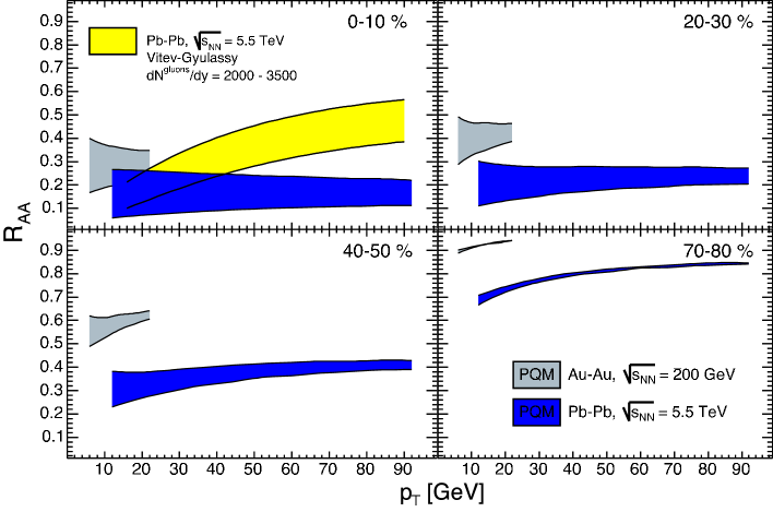
In fig. 33 we report the expected transverse-momentum dependence of $R_{\rm AA}$ at the LHC in the range $10<p_{\mathrm{T}}<90\leavevmode\nobreak\ \mbox{${\rm GeV}$}$ for different centralities; the results at $\sqrt{s_{\scriptscriptstyle{{\rm NN}}}}=200\leavevmode\nobreak\ \mbox{${\rm GeV}$}$ are shown as well. In the most central collisions $R_{\rm AA}$ is of $\approx 0.15$, independent of $p_{\mathrm{T}}$. Our prediction is almost a factor of 2 smaller than the measured value at $\sqrt{s_{\scriptscriptstyle{{\rm NN}}}}=200\leavevmode\nobreak\ \mbox{${\rm GeV}$}$. It is in agreement, both in the numerical value and in the $p_{\mathrm{T}}$-dependence, with [196] using the same quenching weights and the same $\alpha_{\rm S}\left<\hat{q}\right>$, while it is quite different from the calculation by Vitev and Gyulassy [193]. For comparison, we report in the same figure their prediction, which assumes an initial gluon rapidity-density $\mathrm{d}N^{\rm gluons}/\mathrm{d}y$ in the range 2000–3500. They expect $R_{\rm AA}$ to rise significantly at large transverse momenta, from 0.1–0.2 at $20\leavevmode\nobreak\ \mbox{${\rm GeV}$}$ to 0.4–0.6 at $90\leavevmode\nobreak\ \mbox{${\rm GeV}$}$. Note that the difference between the two results is not due to the fact that we do not include nuclear (anti-)shadowing effects, since these are expected to determine a rather $p_{\mathrm{T}}$-independent increase of $R_{\rm AA}$ of about $10$% in the range $25<p_{\mathrm{T}}<100\leavevmode\nobreak\ \mbox{${\rm GeV}$}$ [196].

5 Extrapolation to the intermediate RHIC energy

To verify the predictive power of PQM, we recall the recent measurement of the nuclear modification factor for charged hadrons and neutral pions up to transverse momenta of $7$–$8\leavevmode\nobreak\ \mbox{${\rm GeV}$}$ at RHIC for Au–Au collisions at $\sqrt{s_{\scriptscriptstyle{{\rm NN}}}}=62.4\leavevmode\nobreak\ \mbox{${\rm GeV}$}$. The scaling with the initial gluon number-density gives

$$n^{\rm gluons}_{\rm Au-Au,\,62.4\,GeV}\simeq 0.5\times n^{\rm gluons}_{\rm Au-Au,\,200\,GeV}\;,$$ (32)

which leads to $\left<\hat{q}\right>^{\rm 62.4GeV}\simeq 7\leavevmode\nobreak\ \mbox{${\rm GeV}$}^{2}/\mbox{${\rm fm}$}$ and $k^{\rm 62.4GeV}=2.5\cdot 10^{6}\leavevmode\nobreak\ \mbox{${\rm fm}$}$. We use PQM as before, but generate the parton $p_{\mathrm{T}}$ with PYTHIA at $\sqrt{s}=62.4\leavevmode\nobreak\ \mbox{${\rm GeV}$}$.

Figure 34: PQM results for $R_{\rm AA}(p_{\mathrm{T}})$ in central and semi-peripheral Au–Au collisions at $\sqrt{s_{\scriptscriptstyle{{\rm NN}}}}=62.4\leavevmode\nobreak\ \mbox{${\rm GeV}$}$. The preliminary $\pi^{0}$ data ($0$–$10$% centrality class) from PHENIX [201] are added for comparison. The pp reference is the PHENIX ${\rm pp}\to\pi^{0}+X$ parameterization, the error bars on the data points are the combined statistical and $p_{\mathrm{T}}$-dependent systematic errors. The bar centered at $R_{\rm AA}=1$ gives the systematic error on the normalization.

The results are shown in fig. 34, along with preliminary data from PHENIX [201] for neutral pions up to $p_{\mathrm{T}}\approx 7\leavevmode\nobreak\ \mbox{${\rm GeV}$}$ in $0$–$10$% central collisions. For $p_{\mathrm{T}}\,{\buildrel>\over{{}_{\sim}}}\,5\leavevmode\nobreak\ \mbox{${\rm GeV}$}$, we find $R_{\rm AA}\simeq 0.3$, in very good agreement with the data, in central ($0$–$10$%) collisions. For semi-peripheral ($40$–$50$%) collisions we predict a value of $\simeq 0.7$.

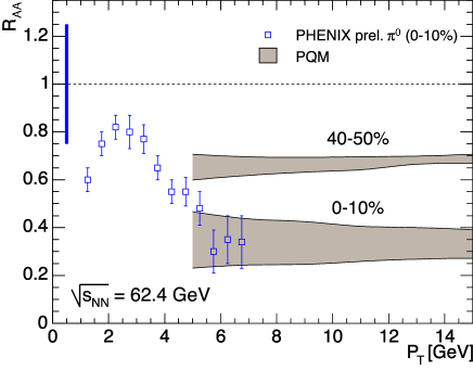
6 Parton emission from the surface

PQM describes the centrality dependence of leading-hadron suppression (see fig. 31) and back-to-back di-hadron correlations (see LABEL:dainese2004) purely by the evolution with the collision geometry. This suggests that the high-opacity medium formed in Au–Au collisions at $\sqrt{s_{\scriptscriptstyle{{\rm NN}}}}=200\leavevmode\nobreak\ \mbox{${\rm GeV}$}$ initially has a size and density, which decrease from central to peripheral events according to the the overlap profile of the colliding nuclei, $T_{\rm A}\,T_{\rm B}(x,y;\,b)$. At the center of the medium the density is highest and partons crossing the central region are likely to be completely absorbed. Only partons produced in the vicinity of the surface and propagating outward can escape from the medium with sufficiently-high energy to fragment into hadrons with more than few ${\rm GeV}$ in $p_{\mathrm{T}}$. Such an “emission from the surface” scenario has also been pictured in LABEL:drees2003, where the centrality dependence of $R_{\rm AA}$ and the back-to-back correlation strength has been reproduced by a simple model of parton absorption whose only physical ingredient was a Glauber-based nucleon–nucleon overlap profile.

Figure 35: Distributions of parton production points in the transverse plane (upper row) and in-medium path length (lower row) for partons that escape the medium and produce hadrons with $p_{\mathrm{T}}>5\leavevmode\nobreak\ \mbox{${\rm GeV}$}$ in central Au–Au collisions at 62.4 and 200 ${\rm GeV}$ and in central Pb–Pb collisions at 5.5 ${\rm TeV}$. The quantity $\left<L\right>$ denotes the average of the path-length distribution. All plots are in the non-reweighted case.

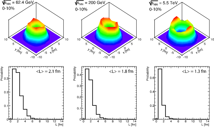
To quantify the effect of surface emission we visualize the region from which partons escape from the medium by plotting the distribution of production points ($x_{0}$, $y_{0}$) for partons fragmenting into high-energy hadrons ($p_{\mathrm{T}}^{\rm hadron}>5\leavevmode\nobreak\ \mbox{${\rm GeV}$}$). The distributions for central Au–Au collisions at $62.4$ and $200\leavevmode\nobreak\ \mbox{${\rm GeV}$}$ and Pb–Pb collisions at $5.5\leavevmode\nobreak\ \mbox{${\rm TeV}$}$ are shown in fig. 35, along with the corresponding in-medium path-length distributions. The “thickness” of the surface is of order $2$–$3\leavevmode\nobreak\ \mbox{${\rm fm}$}$ and it decreases as $\sqrt{s_{\scriptscriptstyle{{\rm NN}}}}$ increases.  The average depth decreases from $\left<L\right>=2.1\leavevmode\nobreak\ \mbox{${\rm fm}$}$ at intermediate RHIC energy, to $1.8\leavevmode\nobreak\ \mbox{${\rm fm}$}$ at $\sqrt{s_{\scriptscriptstyle{{\rm NN}}}}=200\leavevmode\nobreak\ \mbox{${\rm GeV}$}$ and $1.3\leavevmode\nobreak\ \mbox{${\rm fm}$}$ at LHC energy. The reported values are for the non-reweighted case. It is interesting to note that in the reweighted case the ‘surface’ region is much thicker; partons may escape almost from all depths and $\left<L\right>=3\leavevmode\nobreak\ \mbox{${\rm fm}$}$ for all systems. This corresponds to our general statement [1]. The reweighted approach generally simulates a softer transport coefficient, which is not in accordance with the suppression of away-side correlations.

Figure 36: Average relative energy loss versus parton energy for quarks and gluons in central collisions at RHIC (left) and LHC (right) energies for the non-reweighted and reweighted cases.

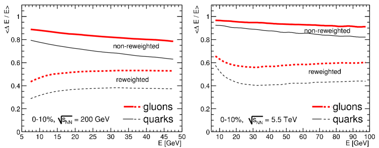
The strong parton absorption in central collisions at RHIC suggests that the saturation regime of the energy loss, $\Delta E/E\to 1$, has been reached. Almost all hard partons produced in the inner core are thermalized ($\Delta E/E=1$) and, thus, cannot escape from the medium. Indeed, the average relative energy loss, $\left<\Delta E/E\right>$, from the Monte Carlo calculation, plotted in fig. 36 as a function of the parton energy $E$ for central collisions at $\sqrt{s_{\scriptscriptstyle{{\rm NN}}}}=200$ and $5500\leavevmode\nobreak\ \mbox{${\rm GeV}$}$, is close to saturation. In the non-reweighted case it reaches $70$–$90$% for gluons and $60$–$80$% for quarks at RHIC and is expected to be even higher at the LHC.  Due to the finite energy constraint and the fact that gluons are closer to energy-loss saturation than quarks, the ratio of gluon to quark $\left<\Delta E/E\right>$ is much smaller than the Casimir ratio $C_{A}/C_{F}=2.25$ expected from eq. (11). Furthermore, since absorption and, hence, saturation is more significant for low-energy partons, or, in other words, since high-energy partons can exploit larger energy losses, the genuine BDMPS-Z $\Delta E/E\propto 1/E$ is replaced by a rather energy-independent effective $\Delta E/E$.

7 Relating the transport coefficient to energy density

The static as well as the time-dependent transport coefficient scale with the energy density of the medium like [156]

$$\hat{q}(\tau)=c\,\epsilon^{3/4}(\tau)\;.$$ (33)

In this expression $c$ is a proportionality constant which is calculated for specific models of the medium. In particular, for ideal QGP interacting perturbatively with the hard parton, the proportionality constant can be extracted from fig. 16 to the value of

$$c_{\rm QGP}^{\rm ideal}\approx 2\;.$$

The time-dependent coefficient for an expanding medium can be written as [159, 155]

$$\hat{q}(\tau)=\hat{q}_{0}\,\left(\tau_{0}/\tau\right)^{\alpha}\;.$$

The expansion parameter $\alpha$ is unity for a one-dimensional Bjorken expansion and is expected to stay close to unity for realistic expansion scenarios. From the measured time-averaged (equivalent static) transport coefficient $\left<\hat{q}\right>$, we find via the dynamical scaling law eq. (13) the transport coefficient for an initial time $\hat{q}_{0}=q(\tau_{0})$

$$\hat{q}_{0}=\hat{q}\,\frac{2-\alpha}{2}\left(\frac{L}{\tau_{0}}\right)^{\alpha}\;,$$ (34)

where we have assumed $\tau_{0}\ll L$. Using this we can calculate the initial energy density, $\epsilon_{0}=\epsilon(\tau_{0})$, according to eq. (33). $L\equiv\tau$ denotes the time at which we extracted the transport coefficient given by the $R_{\rm AA}$ data. Since the measurement is mainly determined by the partons which escape from the medium, we take for $L$ the average value of the path-length distributions depicted in fig. 35. Realistic expansion scenarios lie in the parameter range $0.75<\alpha<1.5$. We chose one-dimensional Bjorken expansion ($\alpha=1$), for which we find the energy densities reported in table 1.

System	$\tau_{0}$ [${\rm fm}$]	$L$ [${\rm fm}$]	$\left<\hat{q}\right>$ [$\mbox{${\rm GeV}$}^{2}/\mbox{${\rm fm}$}$]	$\hat{q}_{0}$ [$\mbox{${\rm GeV}$}^{2}/\mbox{${\rm fm}$}$]	$\epsilon_{0}$ [$\mbox{${\rm GeV}$}/\mbox{${\rm fm}$}^{3}$]
Au–Au  62.4	0.2	2.1	007	037	00715
Au–Au  200	0.2	1.8	014	063	01454
Pb–Pb  5500	0.1	1.3	100	650	32670

Table 1: Initial energy density extracted from eq. (33) and eq. (34) for $c_{\rm QGP}^{\rm ideal}=2$ and $\alpha=1$ (Bjorken expansion). The values for $L$ are taken from fig. 35.

The reported values yield to much larger initial densities compared to the values given by the EKRT model (see tab. 2 on page 2). Note that the calculation of $\hat{q}$ depends on $\alpha_{\rm S}$, for which we chose a rather small value of $1/3$. However, using $\hat{q}=68\leavevmode\nobreak\ \mbox{${\rm GeV}$}^{2}/\mbox{${\rm fm}$}$ (at $\alpha_{\rm S}=0.5$) and an assumed energy density of $\epsilon=100\leavevmode\nobreak\ \mbox{${\rm GeV}$}/\mbox{${\rm fm}$}^{3}$ the value of $c$ at the LHC energy is found to be about $5$–$10$ times larger than perturbatively expected [196]. This is a known and still outstanding problem: The hard probe seems to interact much stronger as expected according to the perturbative estimate. Although this perturbative estimate as well as the theoretical description of parton energy loss at finite (small) parton energies themselves bare significant uncertainties, the authors do not expect them to account for the large discrepancy alone.

8 Limitations due to finite parton energies

The difference between the constrained distributions becomes quite large for low parton energies and sufficiently-large (effective) transport coefficients and (effective) in-medium path lengths. It is controlled by the ratio of the maximum allowed energy loss, $\Delta E^{\rm max}=E$, to the characteristic emission frequency of the gluons, $\omega_{\rm c}$. Mathematically $P^{\rm rw}(\Delta E,\,E)-P^{\rm non-rw}(\Delta E,\,E)$ is largely determined by $(1-\phi(E))/\phi(E)$, where $\phi(E)=\int_{0}^{E}\mathrm{d}\epsilon\,P(\epsilon)$. We evaluate its dependence on $\omega_{\rm c}$ by defining

$$\Phi(z)=\left<\int_{0}^{z}\,\mathrm{d}\xi\,\omega_{\rm c}\,P(\xi\,\omega_{\rm c})\right>$$ (35)

for $z=E/\omega_{\rm c}$. The brackets $\left<\cdot\right>$ in eq. (35) denote the average over the input parameters of the quenching weights, i.e. the average over all parton paths and encountered local transport coefficients determining $\omega_{\rm c}$ via eq. (25).

Figure 37: The accumulated energy-loss probability distribution, eq. (35), averaged over the input parameters of the quenching weights, pairs of $\omega_{\rm c}$ and $R$.

(a) Reweighted

(b) Non-reweighted

Figure 38: The deviation from the unconstrained quenching weights, $1/\Phi(z)$ 38(a) for reweighted and $1-\Phi(z)$ 38(b) for non-reweighted, as a function of $z=E/\omega_{\rm c}$.

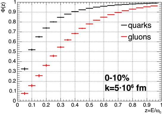
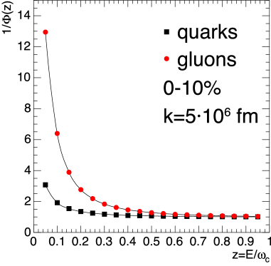
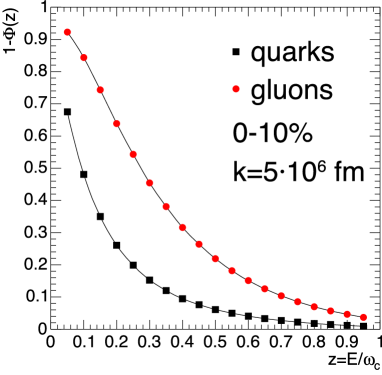
The numerical result of $\Phi(z)$ as a function of $z$ as given by eq. (35) is reported in fig. 37. The remarkable difference between quarks and gluons is due to the broader gluon-radiation distribution (see eq. (10)) for a gluon projectile. Thus, for the same value of $\omega_{\rm c}$ the difference in the two approaches grows for smaller parton energies. 

Furthermore, looking at fig. 38 values of $\Phi(z)\geq 0.5$ are desirable, since $1/\phi(E)$ for the reweighted and $1-\phi(E)$ for the non-reweighted case control to which extent the quenching probabilities calculated in the eikonal approximation are modified by the finite energy constraint. Thus, the parton energy should fulfill $E>0.25\,\omega_{\rm c}$ for quarks and $E>0.5\,\omega_{\rm c}$ for gluons, in order to keep the modification on the weights introduced by the constraints to the $20$% level. For lower values of the initial parton energy relative to the characteristic frequency of the emitted gluons it might not longer be justified to consider multiple successive and independent scatterings of the primary parton in the medium. A similar remark can be found in LABEL:arleo2002.

The current difficulties of the theory to account for finite (small) parton energies become obvious if we compute the distribution of $\omega_{\rm c}$ for central Au–Au collisions shown in fig. 39(a). The mean value of the characteristic emission frequency is very high, $\left<\omega_{\rm c}\right>=870\leavevmode\nobreak\ \mbox{${\rm GeV}$}$ (with large rms of $921\leavevmode\nobreak\ \mbox{${\rm GeV}$}$). The scale is huge compared to the parton energies encountered (surely below $100\leavevmode\nobreak\ \mbox{${\rm GeV}$}$). Quantitatively we can estimate the effect on the constrained weights computing the distribution of $z=E/\omega_{c}$ shown in fig. 39(b). The mean value is $\left<z\right>=0.05$ (with rms of $0.24$), which is below the fraction we quoted above. Thus, for the scale $k=5\cdot 10^{6}\leavevmode\nobreak\ \mbox{${\rm fm}$}$, which fits the nuclear modification factor at RHIC (and further observables as mentioned), we find in view of fig. 38 that basically every $z$-value used is from the $z$-region where the effect of the finite parton energies via the constrained weights is significant: about factor of 2 (quarks) to 6 (gluons) for the reweighted, which is alarmingly high, and about $50$% (quarks) to $90$% (gluons) for the non-reweighted case (taking the value at $z=0.1$).

(a) Distribution of $\omega_{\rm c}$

(b) Distribution of $E/\omega_{\rm c}$

Figure 39: The distribution of $\omega_{\rm c}$ 39(a) and $z=E/\omega_{\rm c}$ 39(b) evaluated with PQM for central Au–Au collisions at $\sqrt{s_{\scriptscriptstyle{{\rm NN}}}}=200\leavevmode\nobreak\ \mbox{${\rm GeV}$}$. The calculation for $k=5\cdot 10^{6}\leavevmode\nobreak\ \mbox{${\rm fm}$}$ results in $\left<\omega_{\rm c}\right>=870\leavevmode\nobreak\ \mbox{${\rm GeV}$}$ and $\left<z\right>=0.05$.

(a) Non-reweighted energy-loss distribution

(b) Reweighted energy loss distribution

Figure 40: Energy loss distribution $P^{\rm non-rw}(\Delta E,\,E)$ 40(a) and $P^{\rm rw}(\Delta E,\,E)$ 40(b) for $E=100\leavevmode\nobreak\ \mbox{${\rm GeV}$}$ partons in central Au–Au collisions at $\sqrt{s_{\scriptscriptstyle{{\rm NN}}}}=200\leavevmode\nobreak\ \mbox{${\rm GeV}$}$. The calculation for $k=5\cdot 10^{6}\leavevmode\nobreak\ \mbox{${\rm fm}$}$ results in $\left<\omega_{\rm c}\right>=870\leavevmode\nobreak\ \mbox{${\rm GeV}$}$ and $\left<R\right>\approx 30000$. See the distribution for lower (fixed) scale in fig. 29.

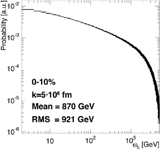
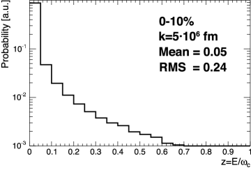
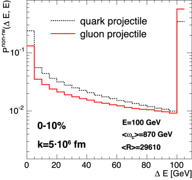
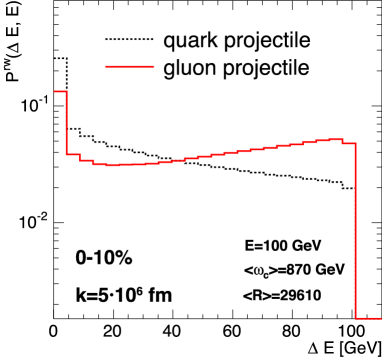
The effect of the high-$\omega_{\rm c}$, i.e. high-$k$ scale, can also be manifested in the energy-loss distribution for fixed parton energies. In fig. 40 it is plotted for $100\leavevmode\nobreak\ \mbox{${\rm GeV}$}$ partons. The average energy loss is $50\leavevmode\nobreak\ \mbox{${\rm GeV}$}$ for quarks and $70\leavevmode\nobreak\ \mbox{${\rm GeV}$}$ for gluons in the non-reweighted; in the reweighted case it is $33\leavevmode\nobreak\ \mbox{${\rm GeV}$}$ for quarks and $50\leavevmode\nobreak\ \mbox{${\rm GeV}$}$ for gluons. This is about $2$–$3$ times larger compared to the distribution obtained for a fixed length (shown in fig. 29). However, what concerns here, is the change of slope in the reweighted case, apparent for gluons relative to quarks in fig. 40(b). The non-reweighted distribution has a peak at zero and at maximal energy loss, as expected by the way it is constructed. Similarly the reweighted distribution has the peak at zero, and for quarks does not possess the peak at maximum possible energy loss, whereas unexpectedly for gluons it does. Due to the high scale needed to describe the data at RHIC the quenching weights are truncated, eq. (27) on page 27, in the rising part of the distribution and then reweighted, thus amplifying the rise. Since the (unconstrained) energy-loss probability distribution for the gluons (shown in fig. 19) is much broader for gluons than for quarks, this occurs for gluons at a lower value of the scale than for quarks.

We, therefore, come to the conclusion to abandon the reweighted approach from further discussion, since at the extrapolated medium-density for RHIC (and even more so for LHC) it introduces substantial deviation from the quenching weights leading to unphysical properties. In addition, it is not in accordance with the observed away-side suppression measured at RHIC. 

9 Limitations of leading-hadron spectroscopy

The expected $R_{\rm AA}$ calculated with PQM in section 4 for central Pb–Pb collisions at LHC as a function of $p_{\mathrm{T}}$ is rather flat, i.e. almost $p_{\mathrm{T}}$-independent. As mentioned, this is in contrast to the estimation by Vitev and Gyulassy [193]. The difference between the two predictions cannot to be attributed to nuclear (anti-)shadowing effects since they are included in a similar calculation [196] coming to the same observation.

In fig. 41 we present the $R_{\rm AA}$ as a function of $p_{\mathrm{T}}$ obtained with PQM in central Pb–Pb at LHC for different settings in the non-reweighted case. Shown are the calculations in the parton-by-parton approach for $k=5\cdot 10^{6}\leavevmode\nobreak\ \mbox{${\rm fm}$}$ (the value found at RHIC), $k=1\cdot 10^{7}\leavevmode\nobreak\ \mbox{${\rm fm}$}$ and $k=4\cdot 10^{7}\leavevmode\nobreak\ \mbox{${\rm fm}$}$ (the value obtained by the scaling from RHIC to LHC), as well as the result of a calculation with fixed $\hat{q}=10\leavevmode\nobreak\ \mbox{${\rm GeV}$}^{2}/\mbox{${\rm fm}$}$ and fixed length of $4.4\leavevmode\nobreak\ \mbox{${\rm fm}$}$ (the mean of the path-length distribution obtained with Glauber). Clearly, the latter shows a stronger $p_{\mathrm{T}}$-dependence than the other cases.

The flatness obtained in the parton-by-parton approach is explained by

• Steeply falling production cross-section, $\propto\left(\frac{1}{p^{\rm hadron}_{\rm T}}\right)^{n(\rm p_{\mathrm{T}})}$, where $n(p_{\mathrm{T}})$ is rising from about $7$ to $12$ (RHIC) and from $6$ to $7$ (LHC) in the relevant $p_{\mathrm{T}}$ regime;

• emission from the surface, which for large medium densities dominates [204].

The computation of $R_{\rm AA}$, eq. (18), at mid-rapidity, can be approximated by [154]

$$R_{\rm AA}(p_{\mathrm{T}})=\left.\int\mathrm{d}\Delta EP(\Delta E,\,p_{\mathrm{T}}+\Delta E)\,\frac{\mathrm{d}N^{\rm pp}(p_{\mathrm{T}}+\Delta E)}{\mathrm{d}p_{\mathrm{T}}}\;\right/\;\frac{\mathrm{d}N^{\rm pp}(p_{\mathrm{T}})}{\mathrm{d}p_{\mathrm{T}}}\;,$$ (36)

where, $\mathrm{d}N^{\rm pp}/\mathrm{d}p_{\mathrm{T}}$ is the spectrum of hadrons (or partons) in the case of no medium (i.e. pp neglecting initial state effects). The suppression computed with eq. (36) is found to give a rather good approximation to the one computed with PQM or with the full formula, eq. (15). In the case the production spectrum is (approximately) exponential the $p_{\mathrm{T}}$-dependence cancels in the ratio and we find $R_{\rm AA}$ to be (approximately) independent of $p_{\mathrm{T}}$. At RHIC this is the case at about $p_{\mathrm{T}}\geq 30\leavevmode\nobreak\ \mbox{${\rm GeV}$}$. Below that value and at the measured values of $5$–$12\leavevmode\nobreak\ \mbox{${\rm GeV}$}$, as well as at the LHC ($n(p_{\mathrm{T}})\leq 7$) the spectrum is given by a power-law and it is expected [154] that $R_{\rm AA}\propto(1+c\,/\sqrt{n(p_{\mathrm{T}})\,p_{\mathrm{T}}})^{-n(p_{\mathrm{T}})}$, i.e. reaching unity in the limit of large $p_{\mathrm{T}}$.

Figure 41: $R_{\rm AA}$ as a function of $p_{\mathrm{T}}$ for $0$–$10$% most central collisions at LHC energy obtained by PQM. The calculations in the parton-by-parton approach (solid lines) are compared to a calculation for fixed transport coefficient and length (dashed). All graphs are in the non-reweighted case.

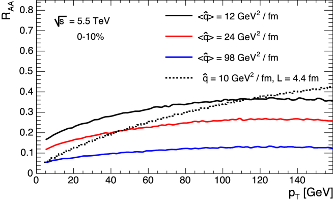
However, this neglects the fact that for dense media surface emission or, more generally, the probability to have no energy-loss, $P(\Delta E=0,\,E)$, plays a significant role, an effect which is even more pronounced at low $p_{\mathrm{T}}$ (compared to $\omega_{\rm c}$). To simplify our argumentation we allow either no loss ($\Delta E=0$) or complete loss ($\Delta E=E$) in the non-reweighted case, $P(\Delta E,\,E)=p_{0}\,\delta(\Delta E)+(1-p_{0})\,\delta(\Delta E-E)$. ^, Inserting the constrained weight into eq. (36) we obtain

$$R_{\rm AA}(p_{\mathrm{T}})=p^{*}+(1-p^{*})\,\left.\frac{\mathrm{d}N^{\rm pp}(2\,p_{\mathrm{T}})}{\mathrm{d}p_{\mathrm{T}}}\,\right/\,\frac{\mathrm{d}N^{\rm pp}(p_{\mathrm{T}})}{\mathrm{d}p_{\mathrm{T}}}\;.$$ (37)

Figure 42: Distributions of parton production points in the transverse plane (upper row) and in-medium path length (lower row) for partons that escape the medium and produce hadrons with $p_{\mathrm{T}}>50\leavevmode\nobreak\ \mbox{${\rm GeV}$}$ in central Pb–Pb collisions at 5.5 ${\rm TeV}$ for $k=5\cdot 10^{6}\leavevmode\nobreak\ \mbox{${\rm fm}$}$ (left) and $k=4\cdot 10^{7}\leavevmode\nobreak\ \mbox{${\rm fm}$}$ (right). The quantity $\left<L\right>$ denotes the average of the path-length distribution. All plots are in the non-reweighted case.

Figure 43: $R_{\rm AA}$ as a function of $\left<\hat{q}\right>$ for $10$ and $100\leavevmode\nobreak\ \mbox{${\rm GeV}$}$ hadrons in $0$–$10$% central Pb–Pb collisions at $\sqrt{s_{\scriptscriptstyle{{\rm NN}}}}=5.5\leavevmode\nobreak\ \mbox{${\rm TeV}$}$. The calculation is done with PQM in the parton-by-parton approach for the non-reweighted case.

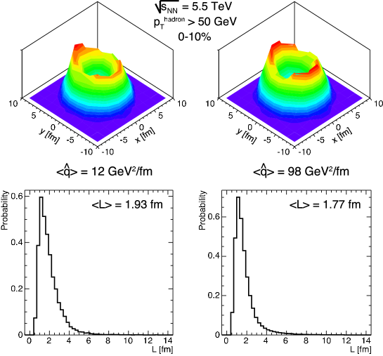
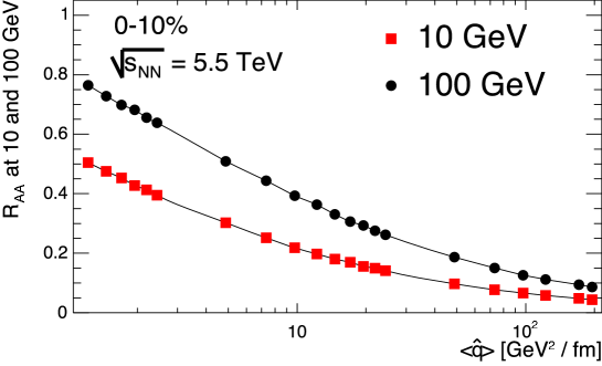
It is obvious that eq. (37) is just a crude approximation, but it demonstrates that the value of $R_{\rm AA}$ is dominated by the fraction of hadrons (or partons), which escape without losing much of their energy. For the simple power-law production spectrum the contribution from higher $p_{\mathrm{T}}$ is suppressed by about $(1+\Delta E/p_{\mathrm{T}})^{n(p_{\mathrm{T}})}$. Taking into account only fixed values of $\hat{q}$ and $L$ the probability $p^{*}$ is given by the discrete weight, $p_{0}$, at $R=0.5\,\hat{q}\,L^{3}$. Note that for a proper calculation one must take into account the right production ratio of quarks-to-gluons.  For realistic path-length distributions $p^{*}$ is dominated by partons, which are emitted close to the surface and, thus, enhanced relative to $p_{0}$ obtained at fixed scale. It turns out that $p^{*}$ evaluated at LHC central conditions, on average over path-lengths and parton types, is independent of $p_{\mathrm{T}}$ in the range shown above, and takes values of about $0.14$, $0.1$ and $0.05$ for the scales used in fig. 41.

To visualize the surface-emission scenario for high-$p_{\mathrm{T}}$ hadrons at LHC we show in fig. 42 (top) the region from which partons escape from the medium by plotting the distribution of production points ($x_{0}$, $y_{0}$) for partons fragmenting into high-energy hadrons with $p_{\mathrm{T}}^{\rm hadron}>50\leavevmode\nobreak\ \mbox{${\rm GeV}$}$ together with the corresponding in-medium path-length distributions (bottom). The chosen values of the scale correspond to the delimiting cases shown in fig. 41 of low and high transport coefficient. Compared to fig. 35 (right) for $p_{\mathrm{T}}^{\rm hadron}>5\leavevmode\nobreak\ \mbox{${\rm GeV}$}$ the “thickness” of the emission surface is larger (about 50%) reaching almost $2\leavevmode\nobreak\ \mbox{${\rm fm}$}$. However, compared to the size of the overlap region, even at LHC hadrons with $p_{\mathrm{T}}>50\leavevmode\nobreak\ \mbox{${\rm GeV}$}$ are emitted dominantly from the surface.

To the present knowledge of the theory (BDMPS-Z-SW) the dominance of the surface effect limits the sensitivity of the $R_{\rm AA}$ to the density of the medium, mainly for experimentally accessible low-$p_{\mathrm{T}}$ range at RHIC. This is demonstrated in fig. 43 where we show the dependence of $R_{\rm AA}$ as a function of the average transport coefficient evaluated with PQM in the parton-by-parton approach for $0$–$10$% most central collisions at $\sqrt{s_{\scriptscriptstyle{{\rm NN}}}}=5.5\leavevmode\nobreak\ \mbox{${\rm TeV}$}$. For $10\leavevmode\nobreak\ \mbox{${\rm GeV}$}$ hadrons the nuclear modification factor is sensitive to average medium densities up to about $15\leavevmode\nobreak\ \mbox{${\rm GeV}$}^{2}/\mbox{${\rm fm}$}$, but loses its sensitivity for higher values of $\left<\hat{q}\right>$. For $100\leavevmode\nobreak\ \mbox{${\rm GeV}$}$ hadrons the sensitive regime might widen to average values of about $50$. 

In most, if not all, cases high-$p_{\mathrm{T}}$ hadrons are leading particles of high-energy jets carrying, on average, 1/3 of the jet energy (section 5). Therefore, the natural extension to leading-hadron spectroscopy is to investigate in-medium modification of well-known jet properties and hadro-production of particles, which are associated with high-$p_{\mathrm{T}}$ trigger (or leading) particles, reported in chapter 5.

Chapter 3 ALICE experimental capabilities

A Large Ion Collider Experiment (ALICE) is a general-purpose experiment whose detectors measure and identify hadrons, electrons, photons, and muons at the LHC. The ALICE detectors are optimized for the study of heavy-ion collisions up to the highest energy available. As such, the detector system has been designed to be capable of measuring properties of the bulk (soft hadronic, large cross section, physics) and of rare probes (hard, small cross section, physics). In particular, ALICE has to be able to track and identify particles from very low, $\sim 100\leavevmode\nobreak\ \mbox{${\rm MeV}$}$, up to fairly high, $\sim 100\leavevmode\nobreak\ \mbox{${\rm GeV}$}$, transverse momenta in an environment of extreme particle density. 

1 Layout of the detector system

The layout of the ALICE detector —as proposed initially together with the physics objectives— is described in the ALICE technical proposal [19] and in two subsequent addenda [205, 206]. The individual detector or sub-detector systems are described in detail in technical design reports and addenda [207, 208, 209, 210, 211, 212, 213, 214, 215, 216, 217, 218, 219]. The addenda reflect modifications to the original design considerations to meet new experimental objectives given by the recent results from RHIC and latest theoretical developments. A summary of the present status of the ALICE detectors can be found in LABEL:pprvol1.

As shown in fig. 1, the ALICE setup consists of three major parts:

• The central barrel contained inside the magnet with an acceptance in pseudo-rapidity of $-0.9\leq\eta\leq 0.9$ over the full azimuth angle;

• the muon spectrometer at the pseudo-rapidity interval $-4.0\leq\eta\leq-2.4$;

• various multiplicity detectors at $-3.4\leq\eta\leq 5.1$.

Figure 1: The ALICE experiment in its final layout. For the sake of visibility the High-Momentum Particle Identification Detector (HMPID) detector is shown in the 12 o’clock position instead of the 2 o’clock position at which it is actually located.

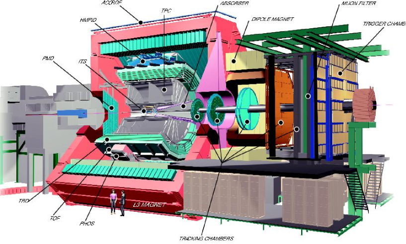
Hadrons, electrons and photons are detected and identified by a complex system of detectors placed in a homogeneous magnetic field of $0.5$ T surrounding the central barrel at $-0.9\leq\eta\leq 0.9$. Charged particle tracking relies on a set of high-granularity detectors: an Inner Tracking System (ITS) consisting of six layers of silicon detectors, a large-volume Time Projection Chamber (TPC), and a high-granularity Transition-Radiation Detector (TRD). Particle identification is performed by measuring the energy loss via ionization (d$E$/d$x$) in the tracking detectors, the transition radiation in the TRD and the time of flight with a high-resolution Time Of Flight (TOF) detector. Two smaller single-arm detectors complete the particle identification at mid-rapidity via the detection of Cherenkov radiation with an HMPID, and photons in the Photon Spectrometer (PHOS) using an electromagnetic calorimeter based on scintillating crystals.

The detection and identification of muons or muon pairs from the decay of heavy quarkonia at $-4.0\leq\eta\leq-2.4$ is performed with a dedicated spectrometer including a warm dipole magnet.

Last but not least, additional detectors located at large rapidities are used to characterize the event and to provide fast interaction triggers. Multiplicity detection by the FMD, V0 and T0 detectors covers a wide acceptance of $-3.4\leq\eta\leq 5.1$ for the measurement of charged particles and triggering, supported by the Photon Multiplicity Detector (PMD) at $2.3\leq\eta\leq 3.5$ for photon multiplicity measurement. Finally the Zero-Degree Calorimeters counts the spectator nucleons in heavy-ion collisions close to the beam rapidity.

For convenience, we will give a brief description of the some of the ALICE detectors in the following sections; for details we refer to the respective technical design reports.

1 Inner Tracking System

The Inner Tracking System (ITS) [207] is designed and optimized for the reconstruction of secondary vertices from hyperon and open-charm (or open-beauty) meson decays, and, thus, precise tracking and identification of low-$p_{\mathrm{T}}$ particles. The detector consists of six cylindrical layers of high resolution silicon detectors, located at the innermost radius of $4\leavevmode\nobreak\ \mbox{${\rm cm}$}$ to the outermost radius of $44\leavevmode\nobreak\ \mbox{${\rm cm}$}$. It covers the rapidity range of $|\eta|<0.9$ for all vertices located within the length of the interaction diamond ($\pm 1\sigma$), i.e.  about $10.6\leavevmode\nobreak\ \mbox{${\rm cm}$}$ along the beam direction.

To cope with the high particle density, up to 80 particles per $\mbox{${\rm cm}$}^{2}$, and to achieve the required impact-parameter resolution of $100\leavevmode\nobreak\ \mu$, pixel detectors have been chosen for the innermost two layers, and silicon drift detectors for the following two layers. The outer two layers, where the track densities are below one particle per $\mbox{${\rm cm}$}^{2}$, are equipped with double-sided silicon micro-strip detectors. The two layers of pixel detectors have about 10⁷ channels with one-bit information (signal above threshold). The silicon drift detectors contain about $1.4\cdot 10^{5}$ channels of 256-deep arrays of digitized 10-bit amplitudes, which are compressed in the front-end electronics. Finally, the strip detectors have $2.6\cdot 10^{6}$ channels of digitized amplitude information.

2 Time Projection Chamber

The Time Projection Chamber (TPC) [208] is the main tracking device of the central barrel. Together with the other barrel detectors, its task is to provide charged-particle momentum measurements and particle identification via energy loss measurements (d$E$/d$x$). The TPC acceptance covers the pseudo-rapidity region of $|\eta|<0.9$; and up to $\left|\eta\right|\sim 1.5$ for tracks with reduced track length and momentum resolution. In $p_{\mathrm{T}}$ up to $100\leavevmode\nobreak\ \mbox{${\rm GeV}$}$ can be measured with good momentum resolution.

The TPC is cylindrical in shape and has an inner radius of about $85\leavevmode\nobreak\ \mbox{${\rm cm}$}$, which is given by the maximum acceptable hit density, and an outer radius of $250\leavevmode\nobreak\ \mbox{${\rm cm}$}$ defined by the length required for a d$E$/d$x$ resolution of $<$10%. Its overall length along the beam direction is $500\leavevmode\nobreak\ \mbox{${\rm cm}$}$. The detector is made of a large field cage, which is divided by a a thin high voltage electrode in the center, providing an uniform electric drift towards the end-caps. It is filled with $88\leavevmode\nobreak\ {\rm m}^{3}$ of Ne/CO₂ (90%/10%), which is needed for the transport of the primary electrons over $2.5\leavevmode\nobreak\ \mbox{${\rm m}$}$ on either side of the central electrode to the end-plates.  The drift gas is optimized for drift speed, low diffusion, low radiation length and hence multiple scattering, small space-charge effect and aging properties.

Multi-wire proportional chambers with cathode pad readout are mounted into 18 trapezoidal sectors of each end-plate, leading to $2\times 18$ trapezoidal sectors, each covering $20^{\circ}$ in azimuth. Due to the radial dependence of the track density, the readout is segmented radially into two type of readout chambers with slightly different wire geometry adapted to the varying pad sizes mentioned below. The inactive areas between neighboring inner chambers are aligned with those between neighboring outer chambers, optimizing the momentum precision for detected high-momentum tracks, but creating cracks in the acceptance, as in about 10% of the azimuthal angle the detector is not sensitive. The readout chambers are made of standard wire planes, i.e. they consist of a grid of anode wires above the pad plane, a cathode wire plane, and a gating grid. Each sector is divided into 6 sub-sectors, sometimes called ‘patches’, four in the outer sector and two in the inner sector. In total, there are $2\times 18\times 6=216$ sub-sectors to be readout.

To keep the occupancy as low as possible and to ensure the necessary d$E$/d$x$ and position resolution, there are about 560 000 readout pads of three different sizes: $4\times 7.5\leavevmode\nobreak\ \mbox{${\rm mm}$}^{2}$ in the inner chambers, $6\times 10\leavevmode\nobreak\ \mbox{${\rm mm}$}^{2}$ and $6\times 15\leavevmode\nobreak\ \mbox{${\rm mm}$}^{2}$ in the outer chambers. The pads are sampled with a frequency of about $5.66\leavevmode\nobreak\ \mbox{${\rm MHz}$}$, dividing the drift time into about 500 time-bins, corresponding to a total drift time of about $88\leavevmode\nobreak\ \mbox{$\mu{\rm s}$}$. Thus, during the drift time about $3\cdot 10^{8}$ 10-bit amplitudes are produced, which subsequently are processed by the TPC front-end electronics [221].

Normally the gating grid protects the readout chambers for electrons coming from the drift volume. The grid only opens after receiving a particular trigger signal (L1, see section 3). This helps to prevent the buildup of space charge from positive ions drifting back from the multiplication region for non-triggered interactions and background.

3 Particle identification detectors

For a large part of the phase space the identification of particles is obtained by a combination of d$E$/d$x$ in the ITS and TPC, and time of flight information from the Time Of Flight (TOF) detector [210, 211].

Electron identification above $1\leavevmode\nobreak\ \mbox{${\rm GeV}$}$ is provided by the Transition-Radiation Detector (TRD) [209], because for momenta greater than $1\leavevmode\nobreak\ \mbox{${\rm GeV}$}$ the pion rejection capability through energy loss measurement in the TPC is no longer sufficient. For quality of electron identification, the TRD consists of six individual layers. Matching the azimuthal segmentation of the TPC, there are 18 sectors. Along the beam direction there is a 5-fold segmentation. Thus, there are $18\times 5\times 6=540$ detector modules. Each module consists of a radiator of $4.8\leavevmode\nobreak\ \mbox{${\rm cm}$}$ thickness and a multi-wire proportional readout chamber including its front-end electronics. Each chamber has about 2000 pads; the pads have a typical area of $6-7\leavevmode\nobreak\ \mbox{${\rm cm}$}^{2}$ and, in total, cover an active area of about $736\leavevmode\nobreak\ m^{2}$ with about $10^{6}$ readout channels. The gas mixture in the readout chambers is Xe/CO₂ (85%/15%). Each readout chamber consists of a drift region of $3.0\leavevmode\nobreak\ \mbox{${\rm cm}$}$; the drift time is $2.0\leavevmode\nobreak\ \mbox{$\mu{\rm s}$}$.The induced signal at the cathode pad plane is sampled in 20 time-bins spaced $1.5\leavevmode\nobreak\ \mbox{${\rm mm}$}$ or $100\leavevmode\nobreak\ \mbox{${\rm ns}$}$ apart. In conjunction with ITS and TPC, the TRD will allow to measure, the production of light and heavy meson resonances in the di-electron channel, as well as to study the di-lepton continuum.

The identification of high-momentum hadrons is provided by the High-Momentum Particle Identification Detector (HMPID) detector [212], which is based on proximity-focusing Ring Imaging Cherenkov (RICH) counters. The detector covers 5% of the acceptance of the central detectors, and extents the identification of hadrons to $p_{\mathrm{T}}\approx 5\leavevmode\nobreak\ \mbox{${\rm GeV}$}$.

Electromagnetic particles are measured by the Photon Spectrometer (PHOS) [213], which is a high-resolution electromagnetic spectrometer with limited acceptance at central rapidity. It provides photon identification as well as neutral meson identification through the two-photon decay channel. The detector is located on the bottom of the ALICE setup, and is built from scintillating lead-tungstate crystals coupled with photo-detectors. It covers approximately a quarter of a unit in pseudo-rapidity, $-0.12\leq\eta\leq 0.12$, and $100^{\circ}$ in azimuthal angle.

It has been proposed [222] to extend the electromagnetic calorimeter coverage of ALICE by a large lead-scintillator sampling Electromagnetic Calorimeter (EMCAL), which will be located between the space frame and the magnetic coils adjacent to HMPID and opposite to PHOS. The detector is foreseen to have a central acceptance in pseudo-rapidity of $\left|\eta\right|\leq 0.7$ with a coverage of $120^{\circ}$ in azimuth and is segmented into $\sim 20000$ towers with a resolution of $\Delta E\sim 15\%/\sqrt{E}$. It will be optimized for the detection of high-$p_{\mathrm{T}}$ photons, neutral pions and electrons, and, together with the barrel tracking detectors, will improve the jet energy resolution.

4 Muon spectrometer

The muon spectrometer [214, 215] is designed to detect muons in the polar angle range $2^{\circ}-9^{\circ}$ ($-4.0\leq\eta\leq-2.5$). It allows to study vector resonances via the $\mu^{+}\mu^{-}$ decay channel. The spectrometer consists of the following components: passive front absorber to absorb hadrons and photons from the interaction vertex; high-granularity tracking system of 10 detection planes; large dipole magnet; passive muon-filter wall followed by four planes of trigger chambers; inner beam shield surrounding the beam pipe to protect the chambers from particles produced at large rapidities.

The design of the tracking system is driven by two main requirements: a spatial resolution of about $100\leavevmode\nobreak\ \mbox{$\mu{\rm m}$}$ and the capability to operate in an high particle-multiplicity environment. The requirements can be fulfilled by the use of cathode pad chambers, which are arranged in five stations: two are placed before, one inside, and two after the dipole magnet. Each station contains two chamber planes, and each chamber contains two cathode planes. Together they provide the two-dimensional hit information. To keep the occupancy at a 5$\%$ level, a large segmentation of the readout pads has been chosen. For instance, pads as small as $4.2\times 6\leavevmode\nobreak\ \mbox{${\rm mm}$}^{2}$ are needed for the region of the first station close to the beam pipe, where the highest multiplicity is expected. Since the hit density decreases with the distance from the beam, larger pads can be used at larger radii. Therefore, the total number of channels can be kept to about $10^{6}$.

5 Multiplicity detectors

Several detector systems placed outside the central barrel will measure global event characteristics such as the event reaction plane, multiplicity of charged particles and precise time and vertex position of the collision. Their combined information can be used to derive the interaction trigger signal.

The Forward Multiplicity Detector (FMD) [216] consists of five silicon-strip ring counters placed on both sides of the interaction point, covering the pseudo-rapidity range $-3.4<\eta<-1.7$ and $1.7<\eta<5.1$ for charged-particle multiplicity measurement. It has in total about $5\cdot 10^{4}$ channels. The readout time of the system is too long to allow the detector to participate in the generation of the low-level trigger information.

The V0 detector [216] is made of two scintillator arrays located asymmetrically on each side of the interaction point. It rejects beam–gas interactions by the time difference between the two arrays, and measures the charged-particle multiplicity using the signal amplitude. The V0 information is used to generate the interaction trigger input and to locate the event vertex.

The T0 detector [216] consists of two arrays of 12 Cherenkov counters each, read out by fine-mesh photo-multiplier tubes. The counters provide the event time with a precision of $50\leavevmode\nobreak\ \mbox{${\rm ps}$}$. The arrays are placed asymmetrically on both sides of the interaction point. The detector is designed to provide the start-time signal for the TOF detector, discriminate against beam–gas interactions and sample particle multiplicity; in addition it provides input for the interaction trigger decision.

The Photon Multiplicity Detector (PMD) [217, 218] is located at $360\leavevmode\nobreak\ \mbox{${\rm cm}$}$ from the interaction point behind the TPC, on the opposite side of the muon spectrometer, and covers the region $2.3<\eta<3.5$. It has about $2.2\cdot 10^{5}$ readout channels; its electronics is similar to that of the muon tracking chambers. The Photon Multiplicity Detector (PMD) is able to measure the ratio of photons to charged particles, the transverse energy of neutral particles, the elliptic flow and the event reaction plane.

Spectator nucleons are detected by means of the Zero-Degree Calorimeters (ZDCs) [219], which are placed at $116\mbox{${\rm m}$}$ from the interaction point, on both sides of the intersection. The ZDCs cannot provide an interaction trigger input in time, since they are located far inside the tunnel. But, using three levels of discrimination they participate in the (later) trigger generation for different centrality classes.

2 Data volume, rate and acquisition

The data volume and data rate, which is produced by the ALICE detectors and their respective front-end electronics, depend on both, the event rate and the event data volume. The event rate is determined by the luminosity of the beam in the collider, while the event data volume is defined by the granularity of the detectors and the particle multiplicity or rather the occupancy in the various detectors.

1 Event rate

The maximum usable luminosity is limited by LHC accelerator complex, by the number of participating experiments and by the dead times of the detectors.

Taking $7.8\leavevmode\nobreak\ \mbox{${\rm b}$}$ for the total (geometrical) cross section, see section 7.A on page 7.A, the event rate for Pb–Pb collisions at the LHC maximum (initial) luminosity of ${\cal{L}}_{0}=10^{27}\leavevmode\nobreak\ \mbox{${\rm cm}^{-2}{\rm s}^{-1}$}$ will be about 8000 minimum-bias collisions per second. This low interaction rate is crucial for the design of the experiment, since it allows to use slow, but high-granularity detectors, such as the time-projection chamber and the silicon drift detectors. The time-averaged luminosity for one participating experiment is $0.44\,\,{\cal{L}}_{0}$ [223]. Thus, throughout the thesis we will use ${\cal{L}}=5\cdot 10^{26}\leavevmode\nobreak\ \mbox{${\rm cm}^{-2}{\rm s}^{-1}$}$ for Pb–Pb collisions, yielding a minimum-bias rate of $4\mbox{${\rm kHz}$}$.

However, the maximum usable luminosity is limited by the readout of the detectors. In particular, at the above event rates the TPC, which is the slowest detector with an readout time of $88\,\mbox{$\mu{\rm s}$}$, has a significant double event fraction. Additional collisions may occur during its readout causing several superimposed events. These pile-up events are typically displaced in the time direction, but contribute to the local track density and the detector occupancy, and consequently lead to an increase of data volume and at the same time to a decrease of tracking performance. The average fraction of double Pb–Pb events during TPC readout is given by $1-\exp(-2\tau\cdot f)=0.5$, where $\tau=88\leavevmode\nobreak\ \mbox{$\mu{\rm s}$}$ is the drift time and $f=8\leavevmode\nobreak\ \mbox{${\rm kHz}$}$ the interaction frequency.  This effect is specific to the TPC as all other sub-detectors have drift or integration times of up to about $5\leavevmode\nobreak\ \mbox{$\mu{\rm s}$}$. Restricting the double event fraction to below 30%, we end up with the past–future protected (‘clean’) minimum-bias rate of $2\leavevmode\nobreak\ \mbox{${\rm kHz}$}$.

The situation is very different in the case of pp running at nominal LHC centre-of-mass energy of $\sqrt{s}=14\leavevmode\nobreak\ \mbox{${\rm TeV}$}$. The maximum machine luminosity, which ALICE can tolerate, is about three orders of magnitude below the design value for the other experiments, ${\cal{L}}^{\rm pp}_{\rm max}=5\cdot 10^{30}\leavevmode\nobreak\ \mbox{${\rm cm}^{-2}{\rm s}^{-1}$}$ [2]. At this luminosity the interaction rate is amounts to $350\leavevmode\nobreak\ \mbox{${\rm kHz}$}$ assuming that the total pp cross section is $70\leavevmode\nobreak\ \mbox{${\rm mb}$}$. Hence, on average the number of pile-up events in the TPC rises to $60\times 1/2$ events; $97$% of the data volume corresponds to unusable partial events. However, the charged particle density in pp collisions is expected to be about $10$ particles per unit of pseudo-rapidity at mid-pseudo-rapidity (see fig. 1 on page 1), resulting in a total of about $2\times 30\times 10=600$ ($900$) tracks within the (extended) TPC acceptance. Clearly, tracking in such a pile-up is feasible, since the occupancy is more than an order of magnitude below the design value of the TPC.

Concerning event rates involving the operation of the TPC, the maximum possible event rate for both minimum-bias Pb–Pb and pp interactions is limited by the maximum TPC gating frequency to approximately $1\leavevmode\nobreak\ \mbox{${\rm kHz}$}$ [208].

For total rate estimates, all LHC experiments have agreed to use an effective time per year of $10^{7}\leavevmode\nobreak\ \mbox{${\rm s}$}$ for pp and $10^{6}\leavevmode\nobreak\ \mbox{${\rm s}$}$ for heavy-ion operation, since the LHC is expected to run essentially in the same yearly mode as the SPS (starting with several months of pp running followed by several weeks of heavy-ion collisions at the end of each year).

2 Event data volume

The event sizes essentially scale linearly with the charged-particle multiplicity and the resulting occupancy in the detectors. Furthermore —although almost too trivial to mention— they strongly depend on the way the detector information is coded.

Given the amount of readout channels, $3\cdot 10^{8}$, the by far highest amount of data is produced by the TPC detector. Simulations indicate that the average occupancy in the TPC will be about 25% for the highest-multiplicity assumption of $\mathrm{d}N_{\mathrm{ch}}/\mathrm{d}\eta=8000$ taken for the design of the detectors [208]. Multiplying the number of channels with the 10-bit Analog Digital Converter (ADC) dynamic range leads to an event size of $375\leavevmode\nobreak\ \mbox{${\rm MB}$}$, which is to be processed by the front-end electronics. By logarithmically compressing the ADC values from $10\leavevmode\nobreak\ \mbox{${\rm bit}$}$ to $8\leavevmode\nobreak\ \mbox{${\rm bit}$}$, the event size will be reduced to about $300\leavevmode\nobreak\ \mbox{${\rm MB}$}$.  In addition, a 45^∘ cone is cut out of the data, since it is problematic to resolve individual tracks that have a low $p_{\mathrm{T}}$and cross the TPC volume under small angles relative to the beam axis. This rejects all particles, which are not in the geometrical acceptance of the outer detectors and reduces the data size further by about 40%. Finally, after zero-suppression and run-length encoding the raw event size is reduced to $75\leavevmode\nobreak\ \mbox{${\rm MB}$}$, while the event size for all detectors is expected to be about $86.5\leavevmode\nobreak\ \mbox{${\rm MB}$}$ [224]. If the experiment is triggering on the 10% most central, past-future protected, Pb–Pb collisions, corresponding to an interaction rate of $200\leavevmode\nobreak\ \mbox{${\rm Hz}$}$, the data rate produced by the front-end will amount to $17\leavevmode\nobreak\ \mbox{${\rm GB/s}$}$ of which the TPC creates about $14.5\leavevmode\nobreak\ \mbox{${\rm GB/s}$}$ alone. Since on average minimum-bias events have a multiplicity of about 20% compared to central events, the minimum-bias rate at the maximum TPC rate of $1\leavevmode\nobreak\ \mbox{${\rm kHz}$}$ amounts to about $21\leavevmode\nobreak\ \mbox{${\rm GB/s}$}$.

Regarding pp interactions, the estimated single, minimum-bias event size of the TPC is approximately $60\leavevmode\nobreak\ \mbox{${\rm kB}$}$ on average. Due to the additional data of the 60 half-complete events the total volume of the pile-up increases the TPC event size to the order of $2.5\leavevmode\nobreak\ \mbox{${\rm MB}$}$. The data volume created by the front-end of the other detectors in the experiment is negligible in that case. Thus, running at the foreseen maximum TPC rate of $1\leavevmode\nobreak\ \mbox{${\rm kHz}$}$ will lead to a total data rate of $2.5\leavevmode\nobreak\ \mbox{${\rm GB/s}$}$ for pp interactions at the maximum tolerable luminosity of $5\cdot 10^{30}\leavevmode\nobreak\ \mbox{${\rm cm}^{-2}{\rm s}^{-1}$}$. It is interesting to note that for a very low luminosity of $10^{29}\leavevmode\nobreak\ \mbox{${\rm cm}^{-2}{\rm s}^{-1}$}$, which might be achievable at the start of the LHC, essentially no pile-up will occur. In that case the rate would drop down to the order of a few   ${\rm MB/s}$.

Collision type	Luminosity	Event rate	Event size	Date rate	Prob. rate
	[${\rm cm}^{-2}{\rm s}^{-1}$]	[${\rm Hz}$]	[${\rm MB}$]	[${\rm GB/s}$]	[${\rm GB/s}$]
Minimum-bias pp	$5\cdot 10^{30}$	$1000$	$\color[rgb]{1,1,1}0\color[rgb]{0,0,0}2.5$	$\color[rgb]{1,1,1}0\color[rgb]{0,0,0}2.5$
Minimum-bias Pb–Pb	$5\cdot 10^{26}$	$1000$	$21.6$	$21.1$	$7.0$
$0$–$10$% central Pb–Pb	$5\cdot 10^{26}$	$\color[rgb]{1,1,1}0\color[rgb]{0,0,0}200$	$86.5$	$16.9$	$5.6$

Table 1: Expected ALICE event and data rates for different LHC runs, limited in rate and dominated in volume by the participating TPC. The event sizes and correspondingly the rates are without compression. The probable data rate corresponds to $\mathrm{d}N_{\mathrm{ch}}/\mathrm{d}\eta=2500$. Central events are past–future protected, without protection the numbers increase by a factor of 2.

Table 1 summarizes the expected event and data rates for different interactions with participating TPC in the readout. For Pb–Pb interactions the result strongly depends on the expected multiplicity. Predictions for the multiplicity in central Pb–Pb collisions at the LHC range at present from 2000 to 6000 charged particles per pseudo-rapidity unit at mid-pseudo-rapidity, while most extrapolations from RHIC data favor values of $2000$–$3000$ (see section 2 on page 2). Thus, the ‘probable’ value for the particle density (RHIC extrapolation) corresponds roughly to one-third of the worst-case assumption leading to rates of the order of $5-7\leavevmode\nobreak\ \mbox{${\rm GB/s}$}$. The event sizes stated in this section are without further compression. It has been shown [225] that a compression factor of about 2 (typically 60%) can be obtained for real and simulated TPC data using entropy encoding methods [226]. Several additional steps of advanced data-reduction methods are envisaged for the TPC [227].

It should be mentioned that other detectors, e.g. the muon spectrometer, can record data at a much higher rate (roughly $2\leavevmode\nobreak\ \mbox{${\rm kHz}$}$). Where it makes sense to improve the statistics for specific trigger channels, groups of detectors might be read out independently.

3 Trigger system

As already indicated in previous sections, the ALICE experiment will operate in different running modes with significantly different characteristics. The trigger system [224] is responsible for the selection of different types of events and controls the readout of the respective detectors when certain criteria are met. The system operates in three different levels: Level 0 (L0), Level 1 (L1) and Level 2 (L2), which have different latencies. Each level corresponds to criteria imposed from different detectors. The selection criteria get tighter as the trigger level increases. Consequently, the rates, at which each trigger level is operated, decrease at higher levels.

L0 and L1 are fixed-latency triggers. The reason for their separation is that in some detectors the front-end electronics requires a strobe very early, and, therefore, a first trigger decision must be delivered $1.2\leavevmode\nobreak\ \mbox{$\mu{\rm s}$}$ after the collision has taken place. The L0 latency is estimated by the expected transmission time in the cables and limited by the dimensions of the detector. In some cases a triggering detector will not be able to send its input in time. Thus, every information which can be gathered and transmitted in $1.2\leavevmode\nobreak\ \mbox{$\mu{\rm s}$}$ is used to make the L0 decision, while those detectors, which take longer, contribute to the L1 trigger, which arrives at the detectors $5.3\leavevmode\nobreak\ \mbox{$\mu{\rm s}$}$ after the L0 ($6.5\leavevmode\nobreak\ \mbox{$\mu{\rm s}$}$ after the collision time). Its latency is given by the expected time ZDC to issue a trigger signal, including a safety margin of 20%.

The main message of the L0 trigger signal is that an interaction has taken place. The trigger input is mainly based on the information from the T0 and V0 counters, but also other detectors, like PHOS, the EMCAL and the (independent) pre-TRD and muon triggers, deliver input.

The L0 trigger ensures the following criteria:

• The interaction vertex must be close the the nominal collision point;

• the forward-backward track distribution of tracks should be consistent with a
  colliding beam–beam interaction;

• the measured multiplicity must exceed a given threshold.

No strong centrality decision is taken at this level, while at L1 centrality requirements based on the ZDC information can be fulfilled. At L1 the fast detectors and pre-triggers (mentioned above) deliver more concrete information about the triggered physics signal. Furthermore, at this time all detectors are strobed. In particular, the TPC gate is opened, which leads to the restriction that the L1 trigger can operate at a maximum frequency of $1\leavevmode\nobreak\ \mbox{${\rm kHz}$}$, if the TPC is to participate in the readout.

The third step, the L2 decision, has a variable latency. It is mainly used to wait for the fulfillment of the past-future protection condition. Three groups of detectors exists:

• Triggering detectors, which need no protection, since, by design, they must be able to respond to each bunch crossing;

• detectors with a required protection time less than $\pm 10\leavevmode\nobreak\ \mbox{$\mu{\rm s}$}$;

• the TPC with a protection interval of $\pm 88\leavevmode\nobreak\ \mbox{$\mu{\rm s}$}$.

During the L2 decision taking time more selective algorithms are applied on the data extracted from the different trigger and detectors. Based on their result an event will be accepted, Level 2 accept (L2a), or rejected, Level 2 reject (L2r). Since the selection algorithms can differ in processing time, the latency of the L2 trigger is not fixed, but has an upper bound as defined by the TPC drift time. After the L2 trigger, the data of the participating detectors are read out from the respective front-end electronics and fed into the DAQ and HLT systems.

4 Data Acquisition system

The Data Acquisation (DAQ) system [224] collects the data from the sub-detectors and assembles the sub-event data blocks into a full event before the complete event is sent to the mass storage. Its architecture is based on conventional PCs connected by a commodity network, most likely TCP over Gigabit Ethernet. The data transfer from the front-end electronics of the detectors is initiated by the L2a trigger. Following, the data are transferred in parallel from the sub-detectors over optical fibers, so called Detector Data Links, into the Local Data Concentratorss, where the sub-event building takes place. The sub-events built in the LDCs are then sent to a single Global Data Concentrator (GDC), where the full event is assembled. The event building is managed by the Event Building and Distribution System (EBDS) running on all DAQ machines. Its main task is to determine the GDC destination for a particular event. The EBDS communicates its decision to the LDCs. The fully assembled events are finally shipped to the mass storage system and from there to the permanent storage system for archiving and further offline analysis.

The DAQ system is designed to be flexible in order to meet the requirements for the different data taking scenarios. Since pp interactions produce a data rate of about 15% compared to Pb–Pb interactions (for the worst-case multiplicity), the requirements on the system are defined by the expected data rate for the heavy-ion mode. In the heavy-ion mode, two main types of events have to be handled. The first type consists of central Pb–Pb events at a relatively low input rate, but with a large event size. The second type consists of events containing a muon pair reported by the trigger, which is read out with a reduced detector subset, including the muon spectrometer. Much higher event rates at quite small event sizes have to be handled in the latter case, of up to $2\leavevmode\nobreak\ \mbox{${\rm kHz}$}$.

In the ALICE proposal [19], the collaboration estimated the bandwidth of $1.25\leavevmode\nobreak\ \mbox{${\rm GB/s}$}$ to mass storage to provide adequate physics statistics. However, depending on the multiplicity, the expected data rate of the ALICE detectors exceeds the foreseen bandwidth by a factor of 4 (probable case) to 12 (worst case) (see table 1). Since the proposal several physics objectives have been refined, regarding rare processes, where higher statistics (of an order of magnitude) is always welcome, and, since the bandwidth cannot be increased (also because of taping costs), the HLT system has been put forward in a serious of notes [228, 229, 230, 231, 232] and is now being constructed [224].

Its task is to reduce the data rate to an acceptable level in terms of DAQ bandwidth and mass storage costs, and, at the same time, provide the necessary event statistics. The idea is accomplished by processing of the data online, almost in real-time, allowing partial or full event reconstruction to select interesting events or sub-events, and/or to compress the data efficiently using data compression techniques. The same strategy has been proven to efficiently increase statistics while decreasing bandwidth and taping costs in the online system of the STAR experiment [233]. To process the complete event online at data rates of $5-20\leavevmode\nobreak\ \mbox{${\rm GB/s}$}$ requires a massive parallel system. The functionality and architecture of the HLT system are topics of the next section.

Logically, the trigger is located between L2 and event building, and, thus, in the data flow between the front-end electronics of the detectors and the event building of the DAQ system. Technically, the data is duplicated on the way to the DAQ system (most likely via optical splitters) and fed into the HLT system, see fig. 2. While waiting for the trigger decision of the HLT, the DAQ may build the complete event, which it will send to mass storage on HLT accept, or disregard on HLT reject.

3 High-Level Trigger system

The High-Level Trigger (HLT) system [224] is designed to reduce the recorded data rate below the limit of the DAQ and mass storage bandwidth, while preserving the ‘interesting’ physics content of the readout data, and, therefore, increasing the event statistics for these observables. It is the only trigger system in ALICE, which can base its decision on the complete event information. Its latency is in principle variable, and only limited by its buffer capacity and that of the event-building system.

In general, data reduction can be accomplished by either reducing the event rate or by reducing the event size (or both). The first case implies that only a fraction of the available events are sent to mass storage. Exactly that had to done without any HLT being present, since the readout rate coming from the detectors would have to be decreased in order to meet the foreseen bandwidth to mass storage. However, by introducing the HLT data is analyzed online and events can be selected on the basis of physics observables other than the hardware triggers deliver. In the latter case, Region of Interest (ROI) are selected and recorded only and/or data compression by modeling techniques are used to reduce the event size itself, and, thus, increase the possible event rate being sent to mass storage. In combination with the fast trigger systems (TRD pre-, muon trigger, PHOS and EMCAL) it is therefore possible to selectively read out the TPC in the region where the respective hardware trigger found an interesting candidate. In the pp mode the main application is the online removal of the additional pile-up events, and, thus reducing the data rate by more than an order of magnitude. In both cases online processing is needed, requiring pattern recognition for the reconstruction of the event or at least parts of it. In the following we differentiate between selection mode and data compression mode.

1 Selection mode

There are two QCD physics domains addressed by ALICE, which can be separated into ‘mostly soft’ and ‘predominantly hard’ with relatively large and small cross sections, respectively. It turns out that analysis of observables related to soft physics requires modest event statistics of a few $10^{6}$ Pb–Pb and about $10^{8}$ pp collisions, whereas systematic analysis of hard signals calls for an additional one or two orders of magnitude, both in Pb–Pb and pp. For example, inclusive production of jets with total transverse energy of more than $150\leavevmode\nobreak\ \mbox{${\rm GeV}$}$, or of the weaker states in the bottonium family, is expected to occur (within the ALICE tracking acceptance) about once every 10⁴ central Pb–Pb collisions. Clearly, it is the latter sector of ALICE physics where the online selection will be required.

The HLT selection mode can be divided into two subclasses: Complete event selection or rejection (trigger), and ROI readout. The latter can be regarded as filtering the unwanted information from the event. Both are based on the online identification of pre-defined physics characteristics. They have to be known and specified in advance; by studying Monte Carlo and recorded events to train and control the operation of trigger/filter. Depending on the topology of the signals, either full or partial event reconstruction is needed.

Hard probes provide to a large degree the most topologically distinct tracking signatures in the TPC. Therefore, most of the online trigger algorithms, investigated so far, are based on online tracking of the TPC data. Further refinement and support will result from using the early time information of the dedicated hardware trigger systems. The different feasible trigger modes envisaged to date are described in detail in LABEL:alicehlt. We will give a brief summary in the following.

Open charm trigger

The measurement of open charm, i.e. of $D$-mesons, in heavy-ion collisions provide a probe, which is sensitive to the collision dynamics at both short and long time scales. This observable is of main interest at LHC energies and its detection and systematic analysis is one of the main goals of the ALICE experiment [199]. It is estimated [234] that for its analysis $2\cdot 10^{7}$ events are needed ($20\leavevmode\nobreak\ \mbox{${\rm Hz}$}$ of central Pb–Pb for $10^{6}$ seconds). If all events are written to tape, 80% (worst case) and 30% (probable case) of the available DAQ bandwidth would be needed for open charm alone. Simulations concentrating on $D^{0}\rightarrow K\pi$ mode show [61] that a signal–to–event of about 1/1000 and a background–to–event of 1/100 should be obtainable in ALICE. The strategy is to detect $D^{0}$-mesons via their characteristic weak decay topology into pions and kaons and to compute the invariant mass of tracks originating from displaced secondary vertices using a sequence of kinematical and impact parameter cuts. The foreseen HLT event-selection strategy proceeds in two steps: Firstly, a momentum filter, applied as it is done in offline, reduces the data volume by a factor of about four. Secondly, an impact-parameter analysis (with very relaxed parameters compared to the offline selection cuts) rejects events with no obvious D⁰ candidate, reducing the data rate further (the concrete reduction factor is not known). It is expected —although proper simulations are outstanding — that HLT can reduce the rate for the open charm program by a factor of 5–10, thus increasing statistics and at the same time releasing DAQ bandwidth.

Di-electron trigger

The yields of $J/\psi$ and $\Upsilon$ production will be important to measure, since, for example, at SPS, $J/\psi$ suppression has played a major role in the discovery of deconfined matter [235].  The bound systems will be reconstructed by their leptonic decay into $e^{+}e^{-}$. The pair will be tracked through the combined barrel, ITS, TPC and TRD. The hardware trigger of the TRD is constructed to trigger on high-$p_{\mathrm{T}}$ tracks by online reconstruction of particle trajectories in the TRD chambers and on the electron candidates by measuring the total energy loss and the depth profile of the deposited energy. However, the true quarkonium trigger rate is small, i.e. the signal rate for $\Upsilon$ is about $10^{-2}\leavevmode\nobreak\ \mbox{${\rm Hz}$}$, and the trigger is dominated by background. The HLT is able to reject background events by using the complete information of the barrel detectors online. Firstly, TRD tracklets will be combined with TPC and ITS tracks. The fit of the combined track allows the momenta of the candidate pair to be determined more precise than by the TRD alone, and, thus, the HLT will reject secondary electrons by sharpening the momentum cut. Secondly, the HLT can improve the identification of the candidate particles using the additional d$E$/d$x$ information of the TPC. Hence, the background from misidentified pions can be reduced. Simulations indicate that event-rate reduction of a factor of $10$ or even more is within reach.

Di-muon trigger

The measurements of the muon spectrometer are complementary to the quarkonia measurements involving the TRD. The spectrometer is designed to detect vector resonances via the $\mu^{+}\mu^{-}$ decay channel. It will run at the highest possible rate in order to record muons with the lowest possible dead time. The spectrometer is built together with an hardware trigger system, which consists of four Resistive Plate Chambers (RPCs) planes arranged in two stations, one meter apart from each other, placed behind the muon-filter wall. The trigger detector participates also in the L0 decision, since the muon tracking stations require the L0 signal for track-and-hold. The task of the muon trigger system is to select events containing a muon pair candidate coming from the decay of $J/\psi$ or $\Upsilon$ resonances. The background is dominated from low-$p_{\mathrm{T}}$ muons from pion or kaon decays. The L0 fires if at least two tracks with opposite charge above a pre-defined $p_{\mathrm{T}}$ threshold are found. The value of the threshold typically is set to either select low-$p_{\mathrm{T}}$ ($>1\leavevmode\nobreak\ \mbox{${\rm GeV}$}$) or high-$p_{\mathrm{T}}$ ($>2\leavevmode\nobreak\ \mbox{${\rm GeV}$}$) muons from the $J/\psi$ and $\Upsilon$ resonances, respectively. However, the coarse-grained segmentation of the dedicated trigger chambers do not allow a sharp $p_{t}$-cut, resulting in a rather large background rate at L0. The $p_{\mathrm{T}}$resolution can be improved by performing an additional tracking step within the HLT system using information from the slower, but more accurate tracking chambers. Thus, a far better trigger selectivity can be achieved. The expected background rejection factor by inclusion of the HLT algorithm is 5 for the low-$p_{\mathrm{T}}$ and 100 for the high-$p_{\mathrm{T}}$ threshold [237].

Jet trigger

In the light of the previous chapter, the study of jets as probes of the strongly interacting QCD matter will be most interesting at LHC energies. However, quite a high number of collected events are required in order to provide the necessary statistics at high jet energy. Estimations based on Glauber scaling from pp collisions indicate that about one jet with $E_{\mathrm{T}}>100\leavevmode\nobreak\ \mbox{${\rm GeV}$}$ is produced per second in minimum-bias Pb–Pb collisions (see next chapter, fig. 3 on page 3). Depending on the setup of the L1 triggering detectors the HLT will be used to either verify the L1 hypothesis or to solely inspect events at L2. Trigger simulations, reported in section 2 on page 2, show that data rates in pp and in Pb–Pb can be reduced by about a factor of $50$ ($100$ for pp), while keeping $1/10$ ($1/5$ for pp) of the events where $E_{\mathrm{T}}>50\leavevmode\nobreak\ \mbox{${\rm GeV}$}$ and slightly more than half of the events with $E_{\mathrm{T}}>100\leavevmode\nobreak\ \mbox{${\rm GeV}$}$. Assuming 100% efficient hardware triggers at L1, which reduce the event rate to a rate that can be tolerated by the TPC, i.e. below $1\leavevmode\nobreak\ \mbox{${\rm kHz}$}$, at total of about $3\cdot 10^{7}$ minimum-bias Pb–Pb events per ALICE year will be recorded, which contain about $1\cdot 10^{6}$ events with $E_{\mathrm{T}}>50\leavevmode\nobreak\ \mbox{${\rm GeV}$}$. Without the help of hardware triggers the rates will be limited by the maximum inspection rate of the TPC, and by a factor of $1/4$ lower. 

Pile-up removal

In the case of pp running, the foreseen running luminosity of $5\cdot 10^{30}\leavevmode\nobreak\ \mbox{${\rm cm}^{-2}{\rm s}^{-1}$}$ will lead to about 60 superimposed, half-complete events within the TPC frame, i.e. 97% overhead in the data stream. The additional piled-up events are displaced along the beam axis and will be disregarded during offline analysis. Using HLT to reconstruct the TPC tracks online, the tracks corresponding to the original (triggered) event are identified, while the tracks belonging to the pile-up events are disregarded from the readout data stream. Although average spacing in time is about $3\leavevmode\nobreak\ \mbox{$\mu{\rm s}$}$, i.e. about $9\leavevmode\nobreak\ \mbox{${\rm cm}$}$ in the TPC, the events are still not necessarily ordered in drift distance because of the variation of the primary vertex position, which will randomize distances. This influences the online capability to identify the sub-event that belongs to the trigger event and sets a limit to the number of pile-up events, which can be handled. Simulations have revealed that an overall event size reduction of 1/10 can be achieved while retaining an efficiency of more than 95% for the primary tracks of the event. The pile-up removal capabilities of the HLT in the pp mode are even more important, since to be triggered physics signals must be identified to belong to the trigger event and not to the pile-up.

2 Data compression mode

The option to compress the readout data online allows to improve the physics capabilities of the experiment without performing selective readout. In principle, the full event rate could be written to mass storage, if a compression factor of about 5–10 can be achieved.

We concentrate again on the TPC detector, since it produces more than 85% of the total event size alone. It has been shown [225], that TPC data by means of loss-less compression techniques can be compressed, at most, by a factor of two. However, the most efficient data compression is expected by using data-modeling compression methods, which are highly adapted to the underlying TPC data. Such compression algorithms exploit the fact that the relevant information is contained in the reconstructed cluster centroids and the track charge depositions, rather in the ADC values, from which they are inferred. Thus, the parameters of the cluster can be stored as deviations from a model. If the model is well adapted to the data (clusters), the resulting bit-rate needed to code the data, will be small. Since the clusters in the TPC critically depend on the track parameters, the reconstructed tracks and clusters can be used to build an efficient model of the data. In contrast to the loss-less coding algorithms mentioned above, this technique does not keep the original data unmodified, since clusters are stored rather than the ADC values, which make the clusters. Recent studies [227] seem to indicate that compression factors of $5$–$10$ could be achieved using such a compression scheme. However, any data compression method, which is not loss-less on the binary level, must be performed with caution to assure the validity of the measured physical observables. Clearly, data-modeling techniques are not to be used in the first years of the experiment, but might be an interesting option for later on.

3 Architecture

The design of the HLT system is driven by the large amount of data it is foreseen to process, the large uncertainty in the expected rate and the complexity of the processing task, which requires a massive parallel, flexible and extensible computing system.

The HLT system is therefore planned to consist of a large PC cluster farm with several hundred (up to a thousand) separate nodes. Its architecture is mainly determined by two constraints. Firstly, the data flow has an inherent granularity and parallelism, which is given by the readout segmentation of the detectors. Secondly, the system is responsible for issuing a trigger decision based on information derived from a partial or complete event reconstruction. Therefore, the reconstructed data finally has to be collected at a global layer, in which the final trigger algorithms are implemented.  Both requirements demand a hierarchical tree-like topology with an high degree of inter-connectivity.

The foreseen data flow architecture is shown in fig. 2. The data is duplicated on the way into the DAQ system and enters the receiving nodes of the HLT system. These Front-End Processors (FEP) constitute the first layer of the HLT system. Each DDL is mounted on a HLT Readout Receiver Card (HLT-RORC), which is a custom designed PCI card hosted by every FEP. Several HLT-RORCs may be placed in one FEP, depending on the bandwidth and processing requirements. Every HLT-RORC is equipped with additional co-processor functionality for designated pre-processing pattern-recognition steps of the data in order to take load off the FEPs. The total number of HLT-RORCs is defined by the readout granularity of the detectors and corresponds to the total number of DAQ Readout Receiver Cards. For the TPC detector, which as the main data source in the experiment is the biggest contributor, the readout is divided into its respective 216 sub-sectors, as mentioned in section 2. Every sub-sector is read out by a single DDL, and, thus, there $216$ fibers are needed for the TPC alone. In total taking into account all detectors there are about $400$ DDLs.

Figure 2: Data flow architecture of the HLT system. The detector raw data is duplicated and received by DAQ and HLT. The architecture is inherent hierarchical, adapted to the parallelism of the data readout and the various tasks of the pattern recognition.

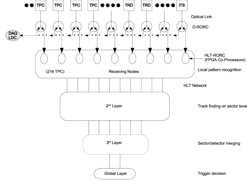
The first pattern recognition step happens while reading the data into the system. It is performed by the Field Programmable Gate Array (FPGA) co-processor hosted on every HLT-RORC. In the case of the TPC local pattern recognition tasks, i.e. cluster finding [238] and/or Hough transformation [239] might be done. The processed data is transferred via the PCI into the main memory of the FEP, where further analysis takes place. From then on the data is an integral part of the HLT communication framework described below. It will —transparently to the FEP and only on request— ship the data to a node of the next processing layer. At every layer there are depending on the type of data and on the processing task to be done as many nodes as necessary to stay within the latency budget. Output data produced by a node of a certain layer is shipped within the communication framework to the next layer until the final stage has been reached. In this way, the processing hierarchy follows a tree-like structure, where successively larger fractions of an event are processed and merged. At the second layer, the processing typically includes track finding within the TPC sectors. At the global level, finally, the necessary fractions have been collected and merged into the reconstructed event, i.e.  tracks from the different sub-sectors are merged and fitted and might be combined with tracks from ITS and TRD. Thus, the complete event (or necessary parts of it) are analyzed by the selection algorithms. The final trigger decision for the event is taken based on the output of the selection algorithms. The decision together with the corresponding data (if any) is transmitted to the DAQ system. The interface between DAQ and HLT is given by a number of DDLs between a set of HLT event merger nodes at the global level and a number of DAQ LDCs.

An essential part of the HLT system is interprocess communication and data transport within the system. A generic communication framework has been developed [240] with emphasis on efficiency in terms of CPU power, flexibility in terms of network topology and fault tolerance regarding failing nodes. The framework implements an interface between different analysis steps (also between different layers) by defining data producers and data consumers. For efficiency data is not communicated between different processes, but rather a descriptor of the data including a reference to the actual data in shared memory is sent. It is therefore ensured that data stays in memory as long as possible, avoiding unnecessary copying (within a single node and over network). The framework basically consists of a number of independent software components, which can be connected together in an arbitrary fashion. The generic interface allows the processing modules to have a common interface which is independent of the underlying transport interface.

Chapter 4 Jets in ALICE

It is our aim to investigate the potential of the ALICE detectors for the measurement of high-energy jets. We start by estimating inclusive single-jet rates in section 1. In section 2 and section 3 we concentrate on the quality of the jet reconstruction at fixed jet energy for various detector settings in pp and Pb–Pb collisions, respectively. In section 1 we present the complete jet spectrum reconstructed by means of offline and online tracking algorithms in pp collisions and discuss the HLT trigger performance. Finally, in section 5 we estimate the yield of back-to-back jet and photon–jet production in the central ALICE acceptance.

1 Expected single-inclusive jet rates

We repeatedly have mentioned the large hard scattering cross section as compared to the geometrical cross section at LHC energies, see section 4 on page 4, which is quantified in the following.

1 Partonic and hadronic cross sections

Using the EKS program [100] we compute the expected inclusive single-jet partonic cross section at mid-pseudo-rapidity for pp collisions at centre-of-mass energies of $1.8$, $5.5$ and $14\leavevmode\nobreak\ \mbox{${\rm TeV}$}$. As reported in section 4 on page 4, the NLO calculation performed at parton level agrees with the measured, and corrected, cross section at highest Tevatron energies of up to $2\leavevmode\nobreak\ \mbox{${\rm TeV}$}$. The values chosen here for the parameters of EKS mostly correspond to the values introduced there, i.e. using a cone of $R=0.7$, a parton separation value of $R_{\rm sep}=1.3$ and all scales at half of the highest jet energy found in the event. Taking CTEQ 5L PDFs is safe, since the obtained cross sections for jet energies between $30\leq E^{\mathrm{jet}}_{\mathrm{T}}\leq 250\leavevmode\nobreak\ \mbox{${\rm GeV}$}$ at mid-rapidity are not sensitive to that choice. For EKS in general, systematic errors are estimated to be about 20% [241]. Note that $x<0.1$, since the discussion is limited to (low) jet energies of less than $250\leavevmode\nobreak\ \mbox{${\rm GeV}$}$, and, thus the large uncertainty in the gluon distribution at high-$x$ does not play a role [115].

Figure 1: Inclusive, partonic single-jet cross section at mid-pseudo-rapidity for pp collisions at centre-of-mass energies of $1.8$, $5.5$ and $14\leavevmode\nobreak\ \mbox{${\rm TeV}$}$ calculated with the EKS program at NLO with the set of parameters as reported in the figure. Compare to fig. 8 on page 8.

Figure 2: Inclusive single-jet cross section at mid-pseudo-rapidity for pp interactions at the LHC centre-of-mass energies of $5.5$ and $14\leavevmode\nobreak\ \mbox{${\rm TeV}$}$ simulated with PYTHIA at LO. The continuous lines show the jet spectrum, identified with the UA1 cone finder for $R=1.0$ using particles in the central ALICE acceptance ($\left|\eta\right|<1$). The dashed lines show the spectrum of the outgoing partons from the hard scattering.

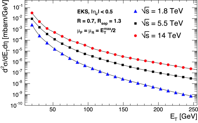
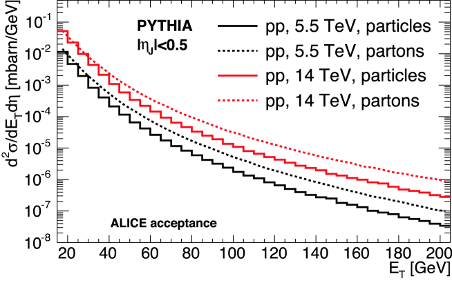
As can be seen in fig. 1, above $50\leavevmode\nobreak\ \mbox{${\rm GeV}$}$ the cross sections at LHC are predicted to be more than an order of magnitude higher than those at high Tevatron energies. With centre-of-mass energy scaling of dimensionless cross-section ratios at the same value of $x_{\mathrm{T}}$

$$R\left(x_{\mathrm{T}}=\frac{2E_{\mathrm{T}}}{\sqrt{s}}=\frac{2E_{\mathrm{T}}^{*}}{\sqrt{s^{*}}}\right)=\frac{E_{\mathrm{T}}^{3}\,\frac{\mathrm{d}\sigma}{\mathrm{d}E_{\mathrm{T}}}(E_{\mathrm{T}},\sqrt{s})}{{E_{\mathrm{T}}^{*}}^{3}\,\frac{\mathrm{d}\sigma}{\mathrm{d}E_{\mathrm{T}}}(E_{\mathrm{T}}^{*},\sqrt{s^{*}})}\approx 1\;,$$ (1)

the value of the cross section may be estimated for higher centre-of-mass energies at corresponding $x_{\mathrm{T}}$ according to

$$\frac{\mathrm{d}\sigma}{\mathrm{d}E_{\mathrm{T}}}\left(\frac{\sqrt{s^{*}}}{\sqrt{s}}\,E_{\mathrm{T}},\sqrt{s}\right)\approx\left(\frac{\sqrt{s}}{\sqrt{s^{*}}}\right)^{3}\,\frac{\mathrm{d}\sigma}{\mathrm{d}E_{\mathrm{T}}}(E_{\mathrm{T}},\sqrt{s^{*}})\;.$$ (2)

The scaling of the ratio, eq. (1), exactly holds in the parton model. For $\sqrt{s}=630$ and $\sqrt{s^{*}}=1800\leavevmode\nobreak\ \mbox{${\rm GeV}$}$, as reported by D0 [242] and Collider Detector at Fermilab (CDF) [87], the scaling is approximately true ($R\leavevmode\nobreak\ \sim 1.5$ at $x_{\mathrm{T}}>0.15$), but uncertainties are large (of up to $50$%); power-like corrections breaking the simple energy scaling must be introduced [243].

Nevertheless, applying eq. (2) with $\mathrm{d}\sigma/\mathrm{d}E_{\mathrm{T}}\sim E_{\mathrm{T}}^{-n}$ gives a value of $\left({\sqrt{s^{*}}}/{\sqrt{s}}\right)^{n-3}$ for the increase of the cross-section ratio at the same value of $E_{\mathrm{T}}$. Taking $n=6$ yields a factor of $30$ at ${\sqrt{s^{*}}}/{\sqrt{s}}=3$ for the extrapolation from $\sqrt{s}=1.8$ to $5.5\leavevmode\nobreak\ \mbox{${\rm TeV}$}$ and about $500$ at ${\sqrt{s^{*}}}/{\sqrt{s}}=7.8$ for the extrapolation to $14\leavevmode\nobreak\ \mbox{${\rm TeV}$}$.

Turning from partons to particles, in fig. 2 we show the corresponding inclusive single-jet cross section at mid-pseudo-rapidity for pp interactions at the LHC centre-of-mass energies of $5.5$ and $14\leavevmode\nobreak\ \mbox{${\rm TeV}$}$ simulated with PYTHIA. The general settings of the simulation are described in section 7.B on page 7.B. The cone finder applied on the particle level with radius of $R=1$ is a variant of UA1 cone finder [96, 97] using the Snowmass accord, eq. (3) on page 3. All particles within the central ALICE acceptance are taken into account, $-1<\eta<1$; no detector response is included. To be accepted in the calculation of the cross section, the jet axis is required to be within the interval $-0.5<\eta_{J}<0.5$ and, thus, the cross section is averaged over the central region. The dashed lines show the corresponding partonic jet-spectrum without ISR and FSR, i.e.the outgoing partons from the hard scattering as calculated by PYTHIA at LO.  At very low jet energy, the cross section measured at particle level almost agrees with the partonic cross section, but, clearly, for higher energy the influence of the detector acceptance reduces the measurable fraction of the (partonic) cross section to about $20$%.

2 Yields at L1 or L2 inspection rate

We are interested in the integrated jet yield at mid-pseudo-rapidity that can be measured with ALICE within a running year. At first, one one may estimate the number of produced jets per second, $N(E_{\mathrm{T}}^{\rm min})$, which at least contain the minimum transverse energy, $E_{\mathrm{T}}^{\rm min}$,

$$N(E_{\mathrm{T}}^{\rm min})={\cal{L}}\,\int_{E_{\mathrm{T}}^{\rm min}}^{\infty}\,\frac{\mathrm{d}\sigma}{\mathrm{d}E_{\mathrm{T}}}\,\mathrm{d}E_{\mathrm{T}}\;.$$ (3)

The average luminosities reported in section 1 on page 1 amount to ${\cal{L}}=0.5\leavevmode\nobreak\ \mbox{${\rm mb}$}^{-1}\mbox{${\rm s}$}^{-1}$ for Pb–Pb and ${\cal{L}}=5\cdot 10^{3}\leavevmode\nobreak\ \mbox{${\rm mb}$}^{-1}\mbox{${\rm s}$}^{-1}$ for pp.  In pp at the two centre-of-mass energies $\frac{\mathrm{d}\sigma}{\mathrm{d}E_{\mathrm{T}}}$ is simply given by the (hadronic) cross section calculated in PYTHIA. For the extrapolation from pp to Pb–Pb at $\sqrt{s_{\scriptscriptstyle{{\rm NN}}}}=5.5\leavevmode\nobreak\ \mbox{${\rm TeV}$}$ we scale $\mathrm{d}\sigma/\mathrm{d}E_{\mathrm{T}}$ according to binary scaling in the Glauber framework, eq. (13) on page 13, with $\sigma^{\rm geo}_{\rm PbPb}=7.8\leavevmode\nobreak\ \mbox{${\rm b}$}$ and $\left<T_{\rm AB}\right>=23.3\leavevmode\nobreak\ \mbox{${\rm mb}$}^{-1}$ for $0$–$10$% central and $\left<T_{\rm AB}\right>=5.5\leavevmode\nobreak\ \mbox{${\rm mb}$}^{-1}$ for minimum-bias collisions, respectively.

Figure 3: Jet yield per second, eq. (3), for jets with $E_{\mathrm{T}}>E_{\mathrm{T}}^{\rm min}$ at mid-pseudo-rapidity in minimum-bias pp collisions at $5.5$ and $14\leavevmode\nobreak\ \mbox{${\rm TeV}$}$, as well as the binary scaled extrapolation for central and minimum-bias Pb–Pb collisions at $\sqrt{s_{\scriptscriptstyle{{\rm NN}}}}=5.5\leavevmode\nobreak\ \mbox{${\rm TeV}$}$. The jet sample corresponds to the spectrum shown in fig. 2.

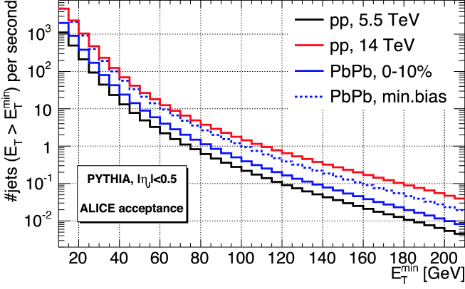
The integrated jet yield per second, eq. (3), is shown in fig. 3 as a function of the minimum energy for minimum-bias pp collisions at $\sqrt{s}=5.5$ and $14\leavevmode\nobreak\ \mbox{${\rm TeV}$}$, as well as for central and minimum-bias Pb–Pb collisions at $\sqrt{s_{\scriptscriptstyle{{\rm NN}}}}=5.5\leavevmode\nobreak\ \mbox{${\rm TeV}$}$. Thus, at $E_{\mathrm{T}}^{\rm min}=100\leavevmode\nobreak\ \mbox{${\rm GeV}$}$, on average, one jet per second will be produced in minimum-bias Pb–Pb collisions at $\sqrt{s_{\scriptscriptstyle{{\rm NN}}}}=5.5\leavevmode\nobreak\ \mbox{${\rm TeV}$}$ and about four in ten seconds for $0$–$10$% most central collisions; the rate in pp at $\sqrt{s}=5.5\leavevmode\nobreak\ \mbox{${\rm TeV}$}$ is about one jet in every two seconds and about one jet per second at $14\leavevmode\nobreak\ \mbox{${\rm TeV}$}$.

It is important to note that for a given centrality the estimated rates are much lower than the L1 trigger rate ($100\leavevmode\nobreak\ \mbox{${\rm kHz}$})$ and for $E_{\mathrm{T}}\geq 30\leavevmode\nobreak\ \mbox{${\rm GeV}$}$ lower than the maximum gating frequency of the TPC ($1\leavevmode\nobreak\ \mbox{${\rm kHz}$})$. Therefore, the total yield per year can be estimated by

$$Y^{\rm year}_{\rm L1}(E_{\mathrm{T}}^{\rm min})=\epsilon_{\rm L1}\,t_{\rm run}\,N(E_{\mathrm{T}}^{\rm min})\;,$$ (4)

where $t_{\rm run}=10^{7}\leavevmode\nobreak\ \mbox{${\rm s}$}$ for pp and $10^{6}\leavevmode\nobreak\ \mbox{${\rm s}$}$ for Pb–Pb denotes the effective running time per year and $\epsilon_{\rm L1}$ is the jet-detection efficiency of the TRD, PHOS and EMCAL (pre-) triggering complex at L1. Of course, in reality the efficiency will depend on $E_{\mathrm{T}}^{\rm min}$. Assuming an optimal trigger, $100$% efficiency for the signal, $\epsilon_{\rm L1}=1$, and low accidental trigger rate compared to $1\leavevmode\nobreak\ \mbox{${\rm kHz}$}$, we end up with the total yields reported for $E_{\mathrm{T}}^{\rm min}=50$, $100$, $150$ and $200\leavevmode\nobreak\ \mbox{${\rm GeV}$}$ in table 1.

Collision type	pp, $5.5\leavevmode\nobreak\ \mbox{${\rm TeV}$}$	pp, $14\leavevmode\nobreak\ \mbox{${\rm TeV}$}$	Pb–Pb, minimum-bias	Pb–Pb, $0$–$10$%
$Y^{\rm year}_{\rm L1}(50\leavevmode\nobreak\ \mbox{${\rm GeV}$})$	$4.9\cdot 10^{7}$	$2.3\cdot 10^{8}$	$2.1\cdot 10^{7}$	$8.9\cdot 10^{6}$
$Y^{\rm year}_{\rm L1}(100\leavevmode\nobreak\ \mbox{${\rm GeV}$})$	$2.2\cdot 10^{6}$	$1.4\cdot 10^{7}$	$9.4\cdot 10^{5}$	$4.0\cdot 10^{5}$
$Y^{\rm year}_{\rm L1}(150\leavevmode\nobreak\ \mbox{${\rm GeV}$})$	$3.0\cdot 10^{5}$	$2.3\cdot 10^{6}$	$1.3\cdot 10^{5}$	$5.4\cdot 10^{4}$
$Y^{\rm year}_{\rm L1}(200\leavevmode\nobreak\ \mbox{${\rm GeV}$})$	$5.4\cdot 10^{4}$	$4.7\cdot 10^{5}$	$2.3\cdot 10^{4}$	$9.8\cdot 10^{3}$

Table 1: Accumulated jet yield per ALICE run year, eq. (4), at mid-pseudo-rapidity for optimum hardware triggers at L1 exploiting the production rate.

The rates estimated above are production rates, i.e. relative to the minimum-bias collision rate, $\leavevmode\nobreak\ {\cal{L}}\,\sigma^{\rm tot}$, which can only be exploited by fast dedicated triggers in hardware. As discussed in section 3 on page 3, the HLT system might be used in addition to the hardware triggers or stand-alone to either verify the L1 hypothesis or to online search for jets using the detector information of the complete event.

Let’s assume for a moment that no other hardware triggers (except from centrality detection) are available. In this case the inspection rate is limited to the maximum gating frequency of $1\leavevmode\nobreak\ \mbox{${\rm kHz}$}$, or lower for past–future protection in central Pb–Pb collisions. Taking for $\sigma^{\rm tot}$ the value of the pp inelastic cross section of $70\leavevmode\nobreak\ \mbox{${\rm mb}$}$ and $79\leavevmode\nobreak\ \mbox{${\rm mb}$}$ [79] and for Pb–Pb the geometrical cross section, $\sigma^{\rm geo}_{\rm PbPb}=7.8\leavevmode\nobreak\ \mbox{${\rm b}$}$, we compute the ratio of maximum TPC inspection rate at L2 over the collision rate, $r_{\rm TPC}$. It is $r_{\rm TPC}=1/350$ and $r_{\rm TPC}=1/400$ for pp at $\sqrt{s}=5.5\leavevmode\nobreak\ \mbox{${\rm TeV}$}$ and $14\leavevmode\nobreak\ \mbox{${\rm TeV}$}$, whereas it is $r_{\rm TPC}=1/4$ for Pb–Pb collisions at $\sqrt{s_{\scriptscriptstyle{{\rm NN}}}}=5.5\leavevmode\nobreak\ \mbox{${\rm TeV}$}$. For the case, the HLT runs without the help of hardware triggers, we define the expected integrated yield per ALICE run year as

$$Y^{\rm run}_{\rm HLT}(E_{\mathrm{T}}^{\rm min})=\epsilon_{\rm HLT}\,r_{\rm TPC}\,t_{\rm run}\,N(E_{\mathrm{T}}^{\rm min})\;,$$ (5)

where $\epsilon_{\rm HLT}$ denotes the efficiency of the HLT jet finder, which depends on $E_{\mathrm{T}}^{\rm min}$.

Assuming $\epsilon_{\rm HLT}=1$ the integrated yield is shown in fig. 4 for minimum-bias pp collisions at $\sqrt{s}=5.5$ and $14\leavevmode\nobreak\ \mbox{${\rm TeV}$}$, as well as for central and minimum-bias Pb–Pb collisions at $\sqrt{s_{\scriptscriptstyle{{\rm NN}}}}=5.5\leavevmode\nobreak\ \mbox{${\rm TeV}$}$. . The total integrated yield for $E_{\mathrm{T}}^{\rm min}=100\leavevmode\nobreak\ \mbox{${\rm GeV}$}$ in minimum-bias Pb–Pb collision amounts to about $2\cdot 10^{5}$; in $0$–$10$% central collisions it is about an order of magnitude lower, on the level of $10^{4}$ events per year and about the same for the reference measurements in pp. These numbers are at the the statistical limit needed for the analysis of jet properties at high-$z$.  Table 2 summarizes the expected total jet yield for $E_{\mathrm{T}}^{\rm min}=50$, $100$, $150$ and $200\leavevmode\nobreak\ \mbox{${\rm GeV}$}$ in the case the HLT inspects the TPC without L1 triggers.

Figure 4: Total jet yield per ALICE run year, eq. (5) with $\epsilon_{\rm HLT}=1$ limited by the TPC inspection rate, for jets with $E_{\mathrm{T}}>E_{\mathrm{T}}^{\rm min}$ at mid-pseudo-rapidity in minimum-bias pp collisions at $5.5$ and $14\leavevmode\nobreak\ \mbox{${\rm TeV}$}$, as well as the binary scaled extrapolation for central and minimum-bias Pb–Pb collisions at $\sqrt{s_{\scriptscriptstyle{{\rm NN}}}}=5.5\leavevmode\nobreak\ \mbox{${\rm TeV}$}$. The corresponding jet production rate is shown in fig. 3.

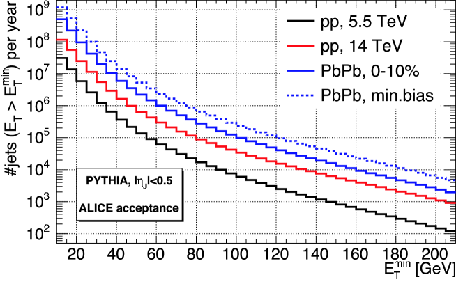
Collision type	pp, $5.5\leavevmode\nobreak\ \mbox{${\rm TeV}$}$	pp, $14\leavevmode\nobreak\ \mbox{${\rm TeV}$}$	Pb–Pb, minimum-bias	Pb–Pb, $0$–$10$%
$Y^{\rm year}_{\rm HLT}(50\leavevmode\nobreak\ \mbox{${\rm GeV}$})$	$1.4\cdot 10^{5}$	$6.4\cdot 10^{5}$	$5.3\cdot 10^{6}$	$2.2\cdot 10^{6}$
$Y^{\rm year}_{\rm HLT}(100\leavevmode\nobreak\ \mbox{${\rm GeV}$})$	$6.1\cdot 10^{3}$	$3.4\cdot 10^{4}$	$2.3\cdot 10^{5}$	$9.8\cdot 10^{5}$
$Y^{\rm year}_{\rm HLT}(150\leavevmode\nobreak\ \mbox{${\rm GeV}$})$	$8.3\cdot 10^{3}$	$5.6\cdot 10^{3}$	$3.2\cdot 10^{4}$	$1.3\cdot 10^{4}$
$Y^{\rm year}_{\rm HLT}(200\leavevmode\nobreak\ \mbox{${\rm GeV}$})$	$1.5\cdot 10^{3}$	$1.1\cdot 10^{3}$	$5.8\cdot 10^{3}$	$2.4\cdot 10^{2}$

Table 2: Accumulated jet yield per ALICE run year, eq. (5) with $\epsilon_{\rm HLT}=1$, at mid-pseudo-rapidity for the case that the HLT runs without dedicated hardware triggers at the maximum TPC inspection rate of $1\leavevmode\nobreak\ \mbox{${\rm kHz}$}$ and at $200\leavevmode\nobreak\ \mbox{${\rm Hz}$}$ in central Pb–Pb collisions.

In practice, of course, ALICE will run with a mix of hardware triggers at L1 and further improve the signal-to-noise ratio by HLT inspection of the triggered events. In this case, the yield will be given by a combination of eq. (4) and eq. (5),

$$Y^{\rm run}(E_{\mathrm{T}}^{\rm min})=\epsilon_{\rm HLT}\,\epsilon_{\rm L1}\,t_{\rm run}\,N(E_{\mathrm{T}}^{\rm min})\;,$$ (6)

and, thus, in the best case, will correspond to eq. (4).

The total rate of accepted events per second,

$$N_{\rm acc}=f_{\rm HLT}\,f_{\rm L1}\,{\cal{L}}\,\sigma^{\rm tot}\;,$$ (7)

is determined by the fraction of accepted events of the involved triggers, $f_{\rm i}$. At L1 the efficiency should be as high as possible, while the rejection of pure background should only reduce the event rate below the TPC readout rate, i.e. around $1/100$ for pp and about $1/5$ for Pb–Pb. The HLT system then must verify the trigger hypothesis and reduce the rate of accepted events below an affordable limit, which will be discussed in section 4.

2 Jet reconstruction in pp for fixed energy

It is instructive to at first start with the jet reconstruction capabilities of ALICE in pp collisions. We generate samples of jets with $E^{\mathrm{jet}}_{\mathrm{T}}=50$, $100$, $150$, $200$ and $250\leavevmode\nobreak\ \mbox{${\rm GeV}$}$ at $\sqrt{s}=5.5\leavevmode\nobreak\ \mbox{${\rm TeV}$}$ using PYTHIA (see section 7.B on page 7.B for parameter settings); every sample contains about 3000 events, and every event contains at least one triggered jet in $\left|\eta\right|<0.5$ ($R=1$) within $\pm 2$% of the required jet energy $E^{\mathrm{jet}}_{\mathrm{T}}$ (also denoted as $E_{\mathrm{T}}^{\rm mc}$).

1 Ideal detector response

For jet reconstruction under ideal conditions we distinguish three types of detectors:

• Ideal detector keeping all particles except neutrinos (ideal detector);

• Ideal charged-particle tracking and electromagnetic calorimeters detecting all charged particles as well as photon radiation and neutral pions (ideal barrel+em);

• Ideal charged-particle tracking detecting all charged particles (ideal barrel).

Without simulating the detailed detector response the detectable particle types, which correspond to the different scenarios, are taken from the Monte Carlo. For a given detector type, these particles must furthermore pass geometrical ($-0.9\leq\eta\leq 0.9$) and kinematical ($0.5\leavevmode\nobreak\ \mbox{${\rm GeV}$}\leq p_{\mathrm{T}}\leq 100\leavevmode\nobreak\ \mbox{${\rm GeV}$}$) cuts. These cuts anticipate that lower momenta in pile-up pp or in Pb–Pb will not be efficiently reconstructed, while for higher momenta the $p_{\mathrm{T}}$-resolution of the barrel tracking detectors will be severely degraded or not measurable. The selected particles are then grouped into jets using the developed cone finder algorithm (see section 7.D on page 7.D) with a cone size of $R=1$. The jets reconstructed that way are subject to be discussed in the following.

Figure 5 shows the average fraction of reconstructed jet energy, $\left<E_{\mathrm{T}}^{\rm rec}/E_{\mathrm{T}}^{\rm mc}\right>$, and the reconstructed energy resolution, $\sigma(E_{\mathrm{T}}^{\rm rec})/\left<E_{\mathrm{T}}^{\rm rec}\right>$, as a function of the jet-trigger energy for the three different cases of ideal particle reconstruction and jet finding. It is obvious that for an ideal detector the average energy fraction is very close to one and the resolution is better than $5$% decreasing to $1$% with increasing jet energy. Using only charged-particle tracking of the barrel detectors, independently of the jet energy a mean of slightly less than $60$% with a constant resolution of about $30$% is obtained, which is close to the value of $\sim 0.6$ realized in nature (isospin conservation plus violating decays). Using information provided by ideal electromagnetic calorimeters the mean increases to about 80% with about $20$% resolution.  It is interesting to note that due to large fluctuations in the ratio of charge-to-neutral or electromagnetic-to-neutral particles the resolution is constant and, thus, not decreasing with jet energy.

(a) Mean energy fraction (ideal)

(b) Energy resolution (ideal)

Figure 5: Average fraction of reconstructed jet energy, $\left<E_{\mathrm{T}}^{\rm rec}/E_{\mathrm{T}}^{\rm mc}\right>$ 5(a), and reconstructed energy resolution, $\sigma(E_{\mathrm{T}}^{\rm rec})/\left<E_{\mathrm{T}}^{\rm rec}\right>$ 5(b), both, as a function of the jet-trigger energy (Monte Carlo) for the different ideal cases. Further details are given in the text.

Figure 6: Spatial resolution of the reconstructed jets, $\sigma(\Delta\phi^{\rm mc}_{J})$ and $\sigma(\Delta\eta^{\rm mc}_{J})$, both, as a function of the jet-trigger energy (Monte Carlo) for the different ideal cases. The spatial differences are measured relative to the direction of the triggered jet, $\Delta\phi^{\rm mc}_{J}=\phi^{\rm rec}_{J}-\phi^{\rm mc}_{J}$ and $\Delta\eta^{\rm mc}_{J}=\eta^{\rm rec}_{J}-\eta^{\rm mc}_{J}$.

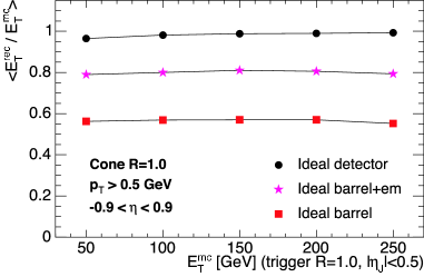
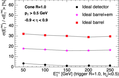
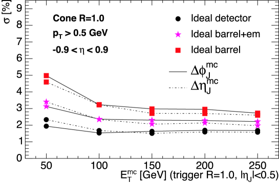
As outlined in section 1 on page 1 it might be important to reconstruct the jet axis accurately enough to resolve the direction of the primary parton from which the jet originates. We define the measured jet axis relative to the triggered jet (which ideally corresponds with the parton direction) and compute the spatial distributions of $\Delta\phi^{\rm mc}_{J}=\phi^{\rm rec}_{J}-\phi^{\rm mc}_{J}$ and $\Delta\eta^{\rm mc}_{J}=\eta^{\rm rec}_{J}-\eta^{\rm mc}_{J}$ for every input energy $E_{\mathrm{T}}^{\rm mc}$ and detector type.  The extracted widths of the Gaussians, which correspond to the spatial resolution of the reconstructed jets, are plotted in fig. 6 as a function of $E_{\mathrm{T}}^{\rm mc}$. As can be seen, $\sigma(\Delta\phi^{\rm mc}_{J})$ and $\sigma(\Delta\eta^{\rm mc}_{J})$ slightly decrease with jet energy. In the ideal case, the resolution is limited by the difference in the definition of the jet finding and jet trigger algorithm and, in general, by intrinsic effects on the parton level. However, most notably, even in the case of charged-particle tracking only, the spatial resolution is better than $5$% at lowest increasing to about $3$% at highest input energy. 

2 Simulated detector response

In the following we estimate the influence of the detector response and of the performance of the different particle-reconstruction methods on jet reconstruction.. The expected detector response may be included in the simulation using the GEANT3 interface of ALIROOT [2]. Based on the assembled hit information the foreseen tracking algorithms can be applied. For the purpose of the thesis we distinguish three cases:

• Charged-particle tracking in the barrel with the offline code using the combined tracking information of ITS, TPC and TRD (offline barrel);

• charged-particle tracking in the TPC with the HLT online code, which is based on cluster finding and track follower (tracker);

• charged-particle tracking in the TPC with the HLT online code, which uses the improved stand-alone Hough transform (hough).

The different methods and in particular their tracking performance have been briefly discussed in chapter 3. As for the ideal cases described above, the tracks (particles) are required to furthermore pass geometrical ($-0.9\leq\eta\leq 0.9$) and kinematical ($0.5\leavevmode\nobreak\ \mbox{${\rm GeV}$}\leq p_{\mathrm{T}}\leq 100\leavevmode\nobreak\ \mbox{${\rm GeV}$}$) selection cuts, before they are grouped into jets using the developed cone finder algorithm (see section 7.D on page 7.D) with a cone size of $R=1$. The reconstructed jets, which are based on charged-particle tracking including simulated detector response, will be discussed in the following and compared to the ideal cases discussed above.

(a) Mean energy fraction (tracked)

(b) Energy resolution (tracked)

Figure 7: Average fraction of reconstructed charged-jet energy, $\left<E_{\mathrm{T}}^{\rm rec}/E_{\mathrm{T}}^{\rm ch}\right>$ 7(a), and reconstructed energy resolution, $\sigma(E_{\mathrm{T}}^{\rm rec})/\left<E_{\mathrm{T}}^{\rm rec}\right>$ 7(b), both, as a function of the jet-trigger energy (Monte Carlo) for the different tracking cases. The corresponding ideal case (ideal barrel) is shown in fig. 5.

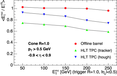
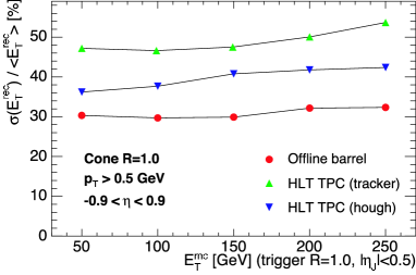
Figure 7 shows the average fraction of reconstructed charged-jet energy, $\left<E_{\mathrm{T}}^{\rm rec}/E_{\mathrm{T}}^{\rm ch}\right>$, and the reconstructed energy resolution, $\sigma(E_{\mathrm{T}}^{\rm rec})/\left<E_{\mathrm{T}}^{\rm rec}\right>$, as a function of the jet-trigger energy for the three different cases of charged-particle reconstruction and jet finding. Opposed to fig. 5, where we take $E_{\mathrm{T}}^{\rm mc}$ of the trigger jet for the normalization, we normalize to the reconstructible charged jet energy (ideal barrel), $E_{\mathrm{T}}^{\rm ch}$. Thus, for offline reconstruction the average fraction of charged-jet energy is very close to the optimum, and, therefore, about $60$% of the total jet energy are, on average, reconstructed. The corresponding resolution is about $30$%, independent of $E_{\mathrm{T}}^{\rm mc}$, and again close to optimal. The online charged-jet energy fraction is decreasing with the trigger-jet energy to about $80$% for the hough and $60$% for the tracker case. In the regime, which due to statistic reasons is most interesting for ALICE, $50$ to $150\leavevmode\nobreak\ \mbox{${\rm GeV}$}$, the average reaches $90$% for hough and about $75$% for the tracker case. The resolution is slightly worse compared to offline, amounting to about $35$–$40$% for hough and about $45$–$55$% for the tracker, which is due to the compromise of tracking efficiency versus running time of the online code. It might be improved once the HLT includes combined tracking using the ITS and TRD detectors in addition to the TPC.

(a) Spatial resolution in $\phi$ (tracked)

(b) Spatial resolution in $\eta$ (tracked)

Figure 8: Spatial resolution of the reconstructed jets, $\sigma(\Delta\phi^{\rm ch}_{J})$ 8(a) and $\sigma(\Delta\eta^{\rm ch}_{J})$ 8(b), both, as a function of the jet-trigger energy (Monte Carlo) for the different tracking cases. The spatial differences are measured relative to the charged jet in the ideal barrel case, $\Delta\phi^{\rm ch}_{J}=\phi^{\rm rec}_{J}-\phi^{\rm ch}_{J}$ and $\Delta\eta^{\rm ch}_{J}=\eta^{\rm rec}_{J}-\eta^{\rm ch}_{J}$. The corresponding ideal case (ideal barrel) is shown in fig. 6.

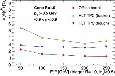
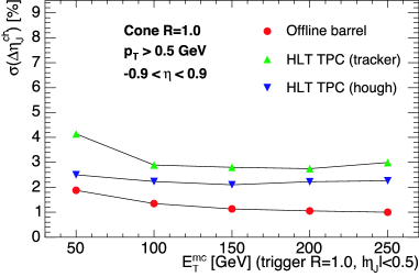
For the estimation of the space resolution we define the measured jet axis relative to the charged jet direction (ideal barrel), $\Delta\phi^{\rm ch}_{J}=\phi^{\rm rec}_{J}-\phi^{\rm ch}_{J}$ and $\Delta\eta^{\rm ch}_{J}=\eta^{\rm rec}_{J}-\eta^{\rm mc}_{J}$. The extracted widths are shown in fig. 8 as a function of $E_{\mathrm{T}}^{\rm mc}$. As expected, the offline combined tracking yields the best resolution of about $2$% (increasing to $1$%), whereas the online Hough track-finder has a constant resolution of $3$% in $\phi$ and $2.5$% in $\eta$ direction. At low Monte Carlo input there is an noticeably difference of almost a factor two between the online tracking based on cluster finding in the TPC and the others, which reduces with increasing input energies.

(a) Spatial resolution in $\phi$ (tracked)

(b) Spatial resolution in $\eta$ (tracked)

Figure 9: Spatial resolution of the reconstructed jets, $\sigma(\Delta\phi^{\rm rec}_{J})$ 9(a) and $\sigma(\Delta\eta^{\rm rec}_{J})$ 9(b), both, as a function of the jet-trigger energy (Monte Carlo) for the different tracking cases. The spatial differences are measured relative to the trigger jet, $\Delta\phi^{\rm rec}_{J}=\phi^{\rm rec}_{J}-\phi^{\rm mc}_{J}$ and $\Delta\eta^{\rm rec}_{J}=\eta^{\rm rec}_{J}-\eta^{\rm mc}_{J}$.

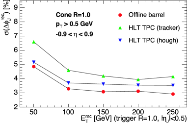
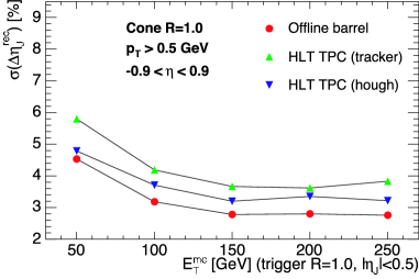
The resolution, $\sigma(\phi_{J}^{\rm rec})$ and $\sigma(\eta_{J}^{\rm rec})$, relative to the trigger jet instead to the charged measured jet could be estimated from fig. 6 and fig. 8 according to

$$\sigma(\phi_{J}^{\rm rec})=\sqrt{\sigma(\phi_{J}^{\rm mc})^{2}+\sigma(\phi_{J}^{\rm ch})^{2}}$$

and similar for $\sigma(\eta_{J}^{\rm rec})$.

For convenience, the resolution is computed directly by comparing the reconstructed jets with the input jets shown in fig. 9. We end up with a jet-reconstruction resolution of about $5$–$7$% at low and $3$–$4$% at high jet energies. However, it is very likely that the resolution in pp collisions will degrade once the additional pile-up events will be taken into account in the simulation.

3 Jet reconstruction in Pb–Pb for fixed energy

Jet reconstruction in Pb–Pb collisions at LHC energies may be affected by the bulk of soft and semi-hard particles, which make up the background, i.e. the ‘underlying event’ in terms of pp physics. As outlined in section 2 on page 2 the expected multiplicity and, thus, also the ‘hardness’ of the background are at present the main unknown. For the estimation of the jet reconstruction capabilities of ALICE in central Pb–Pb collisions we chose HIJING for the generation of background events, in which PYTHIA events containing jet signals are implanted. HIJING, mainly used with default options (section 7.C on page 7.C), generates a rather soft background of about $6000$ charged particles, $2000$ for $p_{\mathrm{T}}>0.5\leavevmode\nobreak\ \mbox{${\rm GeV}$}$, in $\left|\eta\right|<0.5$. Corresponding to the sample of signal events discussed above for pp, we generate 3000 central ($0$–$10$%) background events in which to embed the jets at different energies.

Figure 10: Charged tower configuration in the $\eta$-$\phi$ plane for a $100\leavevmode\nobreak\ \mbox{${\rm GeV}$}$ jet in pp (left) and for the same jet embedded in a central Pb–Pb event (right). In both cases a particle $p_{\mathrm{T}}$-cut of $0.5\leavevmode\nobreak\ \mbox{${\rm GeV}$}$ has been applied.

Figure 11: Distribution of reconstructed (charged) jets found in the signal classes compared to pure background ($0$–$10$% Pb–Pb, HIJING) as a function of the reconstructed energy for the ideal barrel. $R=0.3$ and $p_{\mathrm{T}}\geq 2\leavevmode\nobreak\ \mbox{${\rm GeV}$}$ are used.

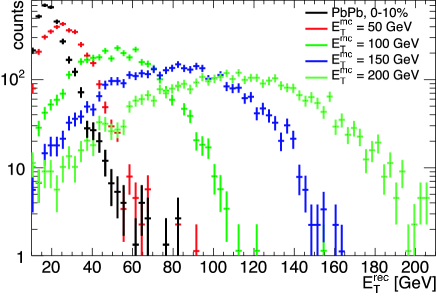
Since, so far, no detector response is simulated, the mixed event contains all particles of the signal and as well of the background event, both, above a $p_{\mathrm{T}}$-cut and within the central ALICE acceptance of $-0.9<\eta<0.9$. The initial tower configuration of the cone finder (section 7.D on page 7.D) is illustrated in fig. 10 for a $100\leavevmode\nobreak\ \mbox{${\rm GeV}$}$ jet in the case of the ideal barrel. Clearly, in the chosen example the signal sticks out of the background (cf.fig. 5 on page 5).

However, for illustration of the situation in the ideal barrel case, we show in fig. 11 the distribution of reconstructed (charged) jets corresponding to the signal classes and pure background as a function of the reconstructed energy. To anticipate the conditions for mixed events (see below) we use $R=0.3$ and $p_{\mathrm{T}}\geq 2\leavevmode\nobreak\ \mbox{${\rm GeV}$}$ for all classes. In the case of the ideal barrel, the distribution arising from pure background partially overlays the distribution arising from jets of about $50\leavevmode\nobreak\ \mbox{${\rm GeV}$}$. Therefore, one qualitatively may expect that the recognition and reconstruction of these, rather low, energy jets within the underlying heavy-ion background will be degraded compared to pure pp. In the following, we will quantify this observation, mainly focusing on the case of ideal barrel tracking (charged particles).

1 Background fluctuations

A single jet with a cone of $R=0.7$ covers $14$% of the ALICE central acceptance. Assuming only about 5000 charged particles with on average $0.5\leavevmode\nobreak\ \mbox{${\rm GeV}$}$ within the acceptance, the expected energy inside the cone amounts on average to about $350\leavevmode\nobreak\ \mbox{${\rm GeV}$}$ arising from uncorrelated background alone.

We start by comparing the average energy content,

$$E_{\mathrm{T}}^{\rm jet}(r)=\frac{1}{\rm N_{\rm jets}}\sum_{\rm jets}E^{\mathrm{jet}}_{\mathrm{T}}(0,r)\;,$$

inside cones of real jets centered at jet axes, cf. eq. (6), with the average content of cones centered at randomly chosen axes in background events,

$$E_{\mathrm{T}}^{\rm bg}(r)=\frac{1}{\rm N_{\rm axes}}\sum_{\rm rand.axes}E_{\mathrm{T}}^{\rm bg}(0,r)\;.$$

(a) Average background

(b) Root mean squared background

Figure 12: Average transverse energy content of $50$ and $150\leavevmode\nobreak\ \mbox{${\rm GeV}$}$ jets, $E_{\mathrm{T}}^{\rm jet}(r)$, compared to the average 12(a) and the rms 12(b) content of randomly chosen cones in the background ($0$–$10$% Pb–Pb, HIJING) as a function of $r$ in the case of ideal barrel. The background is suppressed by $p_{\mathrm{T}}$-cuts of $0.5$, $1$ and $2\leavevmode\nobreak\ \mbox{${\rm GeV}$}$.

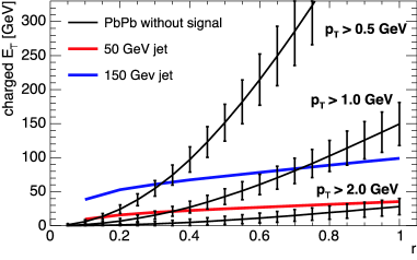
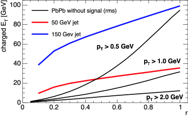
Figure 12 shows the average energy content of $50$ and $150\leavevmode\nobreak\ \mbox{${\rm GeV}$}$ jets compared with the mean and rms of the background as a function of the cone size, $r=\sqrt{(\phi-\phi_{\rm c})^{2}+(\eta-\eta_{\rm c})^{2}}$. The expected behavior of $E_{\mathrm{T}}^{\rm bg}(r)$ to be proportional to $r^{2}$ and its rms, $\Delta E_{\mathrm{T}}^{\rm bg}(r)$, to be proportional to $r$ are approximately true. The $p_{\mathrm{T}}$-cuts of $0.5$, $1$ and $2\leavevmode\nobreak\ \mbox{${\rm GeV}$}$ have been applied to suppress the uncorrelated background. It is obvious that in Pb–Pb at $\sqrt{s_{\scriptscriptstyle{{\rm NN}}}}=5.5\leavevmode\nobreak\ \mbox{${\rm TeV}$}$ one can not apply a cone finder with $R=0.7$ or higher as it is typically done in pp, since for these radii the energy in the jet cone is dominated by the background; furthermore the fluctuations of the background are comparable to the jet energy. Instead, one must reduce the cone size to about $R=0.3$, and, in addition, apply a particle $p_{\mathrm{T}}$-cut of $1$ or $2\leavevmode\nobreak\ \mbox{${\rm GeV}$}$ to resolve jet energies of the order of $50\leavevmode\nobreak\ \mbox{${\rm GeV}$}$ and below. However, the $p_{\mathrm{T}}$-cut is less effective as one would think, since the reduction of the number of low-$p_{\mathrm{T}}$ particles increases the mean and the rms inside the cone (assuming uncorrelated particle production).

Figure 13: The ratio of background fluctuations over jet-signal energy, $\sigma(E_{\mathrm{T}}^{\rm bg})/E^{\mathrm{jet}}_{\mathrm{T}}$, for $50$ and $150\leavevmode\nobreak\ \mbox{${\rm GeV}$}$ jets as a function of $r$ for the case of the ideal barrel. The $p_{\mathrm{T}}$-cuts of $1$ and $2\leavevmode\nobreak\ \mbox{${\rm GeV}$}$ are applied only in the background events ($0$–$10$% Pb–Pb, HIJING).

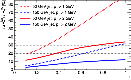
The ratio of the background fluctuations over the jet-signal energy, $\sigma(E_{\mathrm{T}}^{\rm bg})/E^{\mathrm{jet}}_{\mathrm{T}}$, for the $50$ and $150\leavevmode\nobreak\ \mbox{${\rm GeV}$}$ jets as a function of $r$ is shown in fig. 13. Since the jet energy resolution in Pb–Pb is roughly given by the resolution of the jet signal in pp and the fluctuations of the background,

$$\sigma(E_{\mathrm{T}}^{\rm rec})=\sqrt{\sigma(E^{\mathrm{jet}}_{\mathrm{T}})^{2}+\sigma(E_{\mathrm{T}}^{\rm bg})^{2}}\;,$$

one should aim for $\sigma(E_{\mathrm{T}}^{\rm bg})/E^{\mathrm{jet}}_{\mathrm{T}}\leq\sigma(E^{\mathrm{jet}}_{\mathrm{T}})/E^{\mathrm{jet}}_{\mathrm{T}}$. From fig. 5(b) we know that the latter is about $30$% for ideal barrel tracking (and $20$% if ideal electromagnetic calorimetry is included). Thus, in Pb–Pb jet reconstruction at $R=0.3$ with $p_{\mathrm{T}}$-cut of $2\leavevmode\nobreak\ \mbox{${\rm GeV}$}$ seems to be preferable, at least, for a first pass to identify jets (e.g. for the jet trigger in the HLT system). In a second pass for a refined analysis one might increase the cone size and decrease the $p_{\mathrm{T}}$-cut.

2 Out-of-cone fluctuations

So far, we did not consider the effect of the reduced cone size and the $p_{\mathrm{T}}$-cut on the jet signal. Since we are aiming for jet production at mid-pseudo-rapidity, both restrictions are correlated and deteriorate the measured signal. Though it has been shown that for $E^{\mathrm{jet}}_{\mathrm{T}}\geq 50\leavevmode\nobreak\ \mbox{${\rm GeV}$}$ on average $80$% of the charged energy is contained within a cone radius of about 0.3 (cf.fig. 12(b)), on jet-by-jet basis particles produced outside of the reduced cone may significantly degrade the jet-energy resolution.

Figure 14: Out-of-cone fluctuations for fixed $E_{\mathrm{T}}^{\rm mc}=100\leavevmode\nobreak\ \mbox{${\rm GeV}$}$ and cone radii of $R=0.3$, $0.5$, $0.7$ and $1.0$ in the case of an ideal detector. The mean and rms values of the $E_{\mathrm{T}}^{\rm rec}$ distribution are shown in the legend.

Figure 15: Effect of the $p_{\mathrm{T}}$-cut on the reconstructed energy distribution for fixed $E_{\mathrm{T}}^{\rm mc}=100\leavevmode\nobreak\ \mbox{${\rm GeV}$}$ and $R=1.0$ in the case of an ideal detector. The mean and rms values of the $E_{\mathrm{T}}^{\rm rec}$ distribution are shown in the legend.

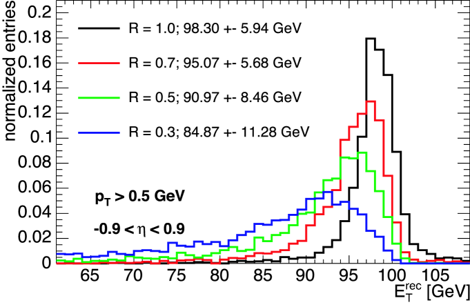
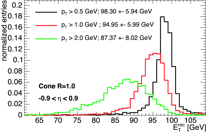
The out-of-cone fluctuations are simplest illustrated by plotting the reconstructed transverse energy distribution, $E_{\mathrm{T}}^{\rm rec}$, for fixed input energy using different radii of the cone finder. As shown in fig. 14 for $E_{\mathrm{T}}^{\rm mc}=100\leavevmode\nobreak\ \mbox{${\rm GeV}$}$ the mean reconstructed values are reduced by up to $15$%; furthermore the distribution is slightly broadened and contains a very long tail to smaller reconstructed energies reaching even zero. Instead, we observe in fig. 15, where for fixed cone radius of $R=1$ the $p_{\mathrm{T}}$-cut varied that the shape of the distribution is preserved, while the mean energy reduces to about the same amount as the out-of-cone fluctuations. Since the shape of the distribution remains Gaussian, the energy resolution is less affected than for reduced cone sizes. It is questionable, whether one should take out-of-cone fluctuations into account for determination of the quality of the jet reconstruction. High-energy jets, which strongly fluctuate to the left, will be overwhelmed by the more likely produced jets at lower energies, and, thus, will simply not be detected; a fact, which contributes to jet detection (in-)efficiency, rather than to the quality of the jet reconstruction algorithm itself.

(a) Mean energy fraction (ideal)

(b) Energy resolution (ideal)

(c) Mean energy fraction (tracked)

(d) Energy resolution (tracked)

Figure 16: Average fraction of reconstructed jet energy, $\left<E_{\mathrm{T}}^{\rm rec}/E_{\mathrm{T}}^{\rm mc}\right>$ 16(a), and corresponding energy resolution, $\sigma(E_{\mathrm{T}}^{\rm rec})/\left<E_{\mathrm{T}}^{\rm rec}\right>$ 16(b), for ideal cases, as well as, average fraction of reconstructed charged-jet energy, $\left<E_{\mathrm{T}}^{\rm rec}/E_{\mathrm{T}}^{\rm ch}\right>$ 16(c), and corresponding energy resolution, $\sigma(E_{\mathrm{T}}^{\rm rec})/\left<E_{\mathrm{T}}^{\rm rec}\right>$ 16(d), for different tracking cases as a function of the jet-trigger energy (Monte Carlo). Opposed to fig. 5 and fig. 7 a cone size of $R=0.3$ and a $p_{\mathrm{T}}$-cut of $2\leavevmode\nobreak\ \mbox{${\rm GeV}$}$ are used. Signal events only without embedding into background are taken.

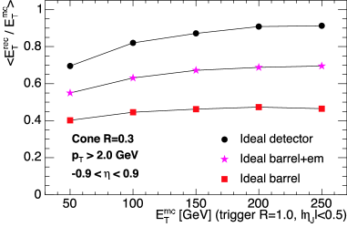
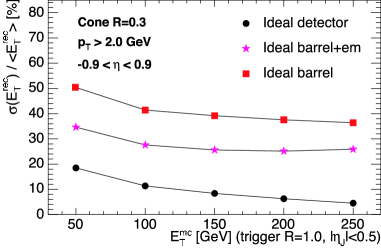
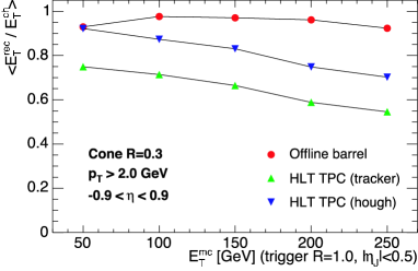
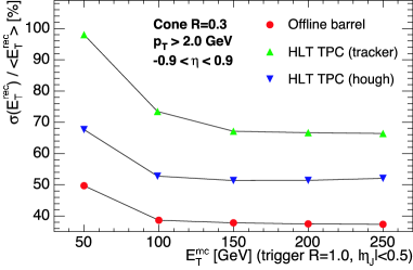
Nevertheless, since in practice jet finding and quality of jet reconstruction are not independent and since one must understand the performance and introduced biases of the online trigger, it is worth to study the impact of the fluctuations in pp at first. Presented in fig. 16 is the combined effect as a function of $E_{\mathrm{T}}^{\rm mc}$ by applying both restrictions, $R=0.3$ and $p_{\mathrm{T}}\geq 2\leavevmode\nobreak\ \mbox{${\rm GeV}$}$, to the samples of signal events (e.g. pp without mixing). The result is quite striking. Even in the case of an ideal detector the mean of the reconstructed jet-energy fraction drops to about $70$% at $50\leavevmode\nobreak\ \mbox{${\rm GeV}$}$, though, as expected, increasing with increasing input energy to the level of $95$%. In the case of ideal barrel tracking the mean reconstructed fraction drops by about $20$% to the level of $40$% (cf. fig. 5). The resolution decreases to about $50$% for $50\leavevmode\nobreak\ \mbox{${\rm GeV}$}$ and about $40$% for the higher energies. Compared to ideal barrel, offline tracking is only slightly affected, but still the overall mean reduces to $37$% with a resolution of $50$% at $E_{\mathrm{T}}^{\rm mc}=50\leavevmode\nobreak\ \mbox{${\rm GeV}$}$. The impact of the additional cuts on the online tracking is more significant (cf. fig. 7). The mean reconstructed energy fraction yields around $35$% ($30$%) at low energies decreasing to $30$% ($25$%), whereas the resolution is about $50$% ($60$%) for the hough (tracker) case. At $E_{\mathrm{T}}^{\rm mc}=50\leavevmode\nobreak\ \mbox{${\rm GeV}$}$ the online resolution degrades to $70$% ($100$%), which might impose a problem for the HLT trigger since jets at that and lower energies are abundantly produced.

(a) Spatial resolution in $\phi$ (tracked)

(b) Spatial resolution in $\eta$ (tracked)

Figure 17: Spatial resolution of the reconstructed jets in signal events only, $\sigma(\Delta\phi^{\rm rec}_{J})$ 17(a) and $\sigma(\Delta\eta^{\rm rec}_{J})$ 17(b), relative to the trigger jet a function of $E_{\mathrm{T}}{\rm mc}$. Opposed to fig. 9 a cone size of $R=0.3$ and a $p_{\mathrm{T}}$-cut of $2\leavevmode\nobreak\ \mbox{${\rm GeV}$}$ are used.

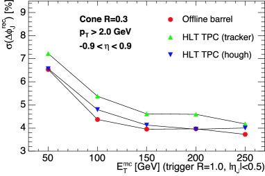
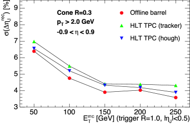
In fig. 17 the spatial resolution, $\Delta\phi^{\rm rec}_{J}$ and $\Delta\eta^{\rm rec}_{J}$, are shown for the signal events (e.g. pp without mixing) in the different tracking cases. Since high-energy jets typically contain at least $8$–$10$ charged particles at high-$p_{\mathrm{T}}$, the spatial resolution only little worsens compared to unconstrained jet reconstruction (cf.fig. 9). The biggest change is again observed at lowest jet energies. There the resolution is about $7$%, but increases to about $4$% at higher energies.

3 Ideal detector response

The findings of the last section refer to pure jet events, i.e. pp only. In this section, we repeat the analysis for signal events, which are embedded into $0$–$10$% central Pb–Pb events. Since for mixed events no realistic detector response is yet available, we use simulations at the Monte Carlo level for the different ideal scenarios defined in section 1.

(a) Mean energy fraction (ideal)

(b) Energy resolution (ideal)

Figure 18: Average fraction of reconstructed jet energy, $\left<E_{\mathrm{T}}^{\rm rec}/E_{\mathrm{T}}^{\rm mc}\right>$ 18(a), and reconstructed energy resolution, $\sigma(E_{\mathrm{T}}^{\rm rec})/\left<E_{\mathrm{T}}^{\rm rec}\right>$ 18(b), both, as a function of the jet-trigger energy (Monte Carlo) for the different ideal cases. The signal jets are embedded into background ($0$–$10$% Pb–Pb, HIJING); $R=0.3$ and $p_{\mathrm{T}}\geq 2\leavevmode\nobreak\ \mbox{${\rm GeV}$}$ are used.

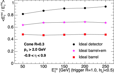
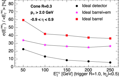
The average fraction of reconstructed jet energy, $\left<E_{\mathrm{T}}^{\rm rec}/E_{\mathrm{T}}^{\rm mc}\right>$, and the energy resolution, $\sigma(E_{\mathrm{T}}^{\rm rec})/\left<E_{\mathrm{T}}^{\rm rec}\right>$, are shown in fig. 18 as a function of the jet trigger energy, $E_{\mathrm{T}}^{\rm mc}$. In order to suppress the background, we $R=0.3$ and $p_{\mathrm{T}}\geq 2\leavevmode\nobreak\ \mbox{${\rm GeV}$}$ are used, as explained in the last section. However, compared to pp with the same cuts (cf. fig. 16(a)) the average mean for the embedded jets still is lifted by the remaining fraction of the underlying event. As expected, the effect is strongest for lowest jet energies; the higher the energy the less the impact of the underlying background fluctuations. Due to the additional fluctuations induced by the underlying event the resolution for the $50\leavevmode\nobreak\ \mbox{${\rm GeV}$}$ jets further degrades (at most $10$% for the ideal barrel), whereas it is almost the same in all other cases.

(a) Ideal detector

(b) Ideal barrel

Figure 19: Distributions of fractions of the jet-signal energy relative to total reconstructed energy for the ideal case 19(a) and the ideal barrel 19(b) as a function of the reconstructed energy, $E_{\mathrm{T}}^{\rm rec}$. The signal jets are embedded into background ($0$–$10$% Pb–Pb, HIJING); $R=0.3$ and $p_{\mathrm{T}}\geq 2\leavevmode\nobreak\ \mbox{${\rm GeV}$}$ are used.

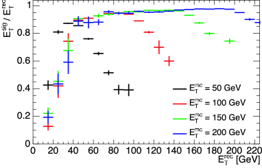
The distribution of energy fraction, which originates from the jet in $R=0.3$, relative to the contribution of the energy due to background inside the jet cone is conveniently reported in fig. 19. Shown for the ideal detector and ideal barrel cases are the fraction of signal energy over the reconstructed energy as a function of the reconstructed energy. Since the mean of the reconstructible fraction from the analysis in pp is known, on average, the reconstructed jet energy arises to about $85$% for $50\leavevmode\nobreak\ \mbox{${\rm GeV}$}$ and about $90$–$95$% for the higher jet energies due to the signal, almost independent of the detector scenario. Opposed to the ideal barrel the contribution of the uncorrelated background to the reconstructed jet energy is clearly apparent for the ideal detector, since neither the jets from the signal, nor the jets from the background are biased to extreme fragmentation into charged particles, only. Note that in the scope of the thesis no attempt has been undertaken to correct for the remaining contribution of the background. 

Figure 20: Spatial resolution of the reconstructed jets, $\sigma(\Delta\phi^{\rm mc}_{J})$ and $\sigma(\Delta\eta^{\rm mc}_{J})$, both, as a function of the jet-trigger energy (Monte Carlo) for the different ideal cases. The spatial differences are measured relative to the direction of the triggered jet, $\Delta\phi^{\rm mc}_{J}=\phi^{\rm rec}_{J}-\phi^{\rm mc}_{J}$ and $\Delta\eta^{\rm mc}_{J}=\eta^{\rm rec}_{J}-\eta^{\rm mc}_{J}$. The signal jets are embedded into background ($0$–$10$% Pb–Pb, HIJING); $R=0.3$ and $p_{\mathrm{T}}\geq 2\leavevmode\nobreak\ \mbox{${\rm GeV}$}$ are used.

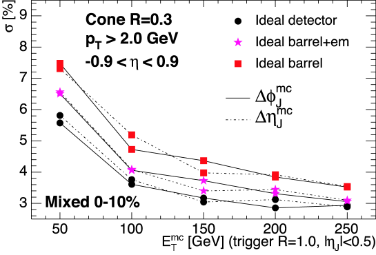
Finally, the spatial resolution of the reconstructed jets in $\phi$-direction, $\sigma(\Delta\phi^{\rm mc}_{J})$, and in $\eta$-direction, $\sigma(\Delta\eta^{\rm mc}_{J})$, as a function of the jet-trigger energy, $E_{\mathrm{T}}^{\rm mc}$, for the different ideal cases is shown in fig. 20. The spatial differences are measured relative to the direction of the triggered jet, $\Delta\phi^{\rm mc}_{J}=\phi^{\rm rec}_{J}-\phi^{\rm mc}_{J}$ and $\Delta\eta^{\rm mc}_{J}=\eta^{\rm rec}_{J}-\eta^{\rm mc}_{J}$. At lowest energy, the mean values are found to amount to about $0.005$ indicating a moderate bias by the background. The resolution for the charged barrel is about $7$–$8$%, which is $2$% worse compared to the resolution obtained in pp with the same constraints on the reconstruction (cf. fig. 17). As expected for higher energies the additional effect of the medium seems not to be apparent.

4 Simulated detector response

It is probably reasonable to assume that high-$p_{\mathrm{T}}$ charged-particle tracking is almost not affected by the underlying soft event. From the analysis of pure signal (pp) events, we know that the offline reconstruction (charged barrel) almost reaches values close to the optimum obtained by the ideal barrel case. In addition, we have shown that the jet-reconstruction performance is dominated by out-of-cone and background fluctuations. Therefore, we expect to reach a spatial resolution of around $10$% with a mean and width of about $50$% of the jet energy once the complete detector response is included.  The inclusion of the EMCAL is expected to improve the mean by about $10$ percent points and the resolution by about $20$ percent points, an expectation which is in accordance with LABEL:blyth2004.

4 Reconstructed jet spectra and trigger rates

After the reconstruction capabilities of the ILCA cone finder have been characterized for different detector scenarios at fixed input jet energies, we will discuss its performance for the realistic spectrum.

1 Single-inclusive jet spectra in pp

We generate the input jet spectrum with PYTHIA at $\sqrt{s}=5.5\leavevmode\nobreak\ \mbox{${\rm TeV}$}$ using 10000 events per $p_{\mathrm{T}}^{\rm hard}$ interval in the way described in section 7.B on page 7.B. Therefore, the distribution of jets given to the simulation framework is distributed according to the cross section shown in fig. 2.

(a) Reconstructed spectrum (ideal)

(b) Reconstructed spectrum (tracked)

Figure 21: Inclusive single-jet cross section at mid-pseudo-rapidity for ideal 21(a) and charged-particle tracking cases 21(b) as a function of the reconstructed jet energy in pp collisions at $\sqrt{s}=5.5\leavevmode\nobreak\ \mbox{${\rm TeV}$}$. The transverse energy is not corrected for introduced biases or inefficiencies of the tracking. The inset shows the ratio of the spectrum obtained by the different tracking methods to the spectrum obtained by the ideal barrel case. All cases are for a cone of $R=0.7$ and $p_{\mathrm{T}}>0.5\leavevmode\nobreak\ \mbox{${\rm GeV}$}$. The input distribution is the same as in fig. 2 and the corresponding cross section agrees with the cross section deduced in the ideal detector case.

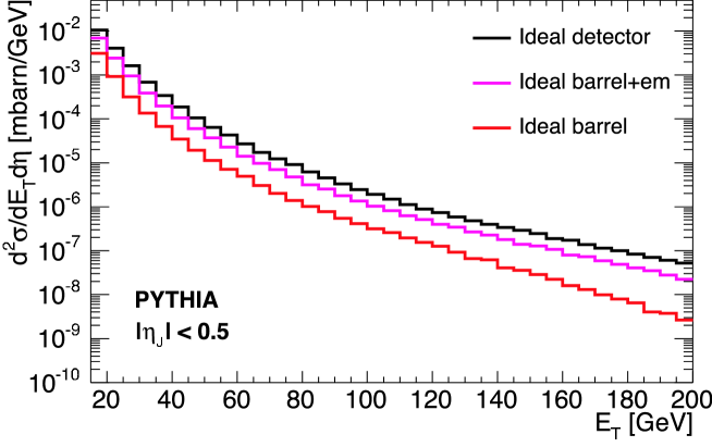
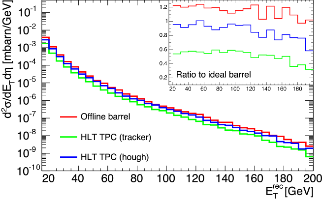
As explained in the previous sections, in the ideal detector cases we just keep the detectable particle types from the Monte Carlo, which correspond to the different scenarios (ideal detector, ideal barrel plus electromagnetic calorimeter and ideal barrel). The spectrum or rather the deduced cross section, reconstructed with the developed ILCA cone finder using $R=0.7$ and $0.5<p_{\mathrm{T}}<100\leavevmode\nobreak\ \mbox{${\rm GeV}$}$, is shown in fig. 21(a) for the ideal cases as a function of the reconstructed transverse jet energy, $E_{\mathrm{T}}^{\rm rec}$, averaged over $\left|\eta\right|<0.5$. The reconstructed energies are not corrected for introduced biases by the different detector types. Especially for the higher energies one notices that the cross section estimated merely based on the ideal barrel detectors underpredicts the real cross section by about one order of magnitude. However, on average, one may correct the obtained cross section by dividing the reconstructed energy with the reconstructible fraction, $0.60$. The corrected distribution corresponds to the spectrum found with the ideal detector within a few percent. As expected from the discussion in the previous sections the inclusion of the EMCAL improves the resolution of the jet energy and, therefore, the determination of the cross section. Without correction, in this case the reconstructed cross section is merely little below the ideal measurement (and the input). But more importantly, it not only allows one to improve the average and jet-by-jet resolution, but also to trigger on neutral particles in the fragmentation of jets.

Since we are dealing with pp events, we include the detailed detector response of the barrel detectors in the simulation and apply the tracking algorithms onto the digitized hit information in the ALIROOT framework (offline barrel, HLT tracker, HLT hough). The reconstructed tracks with $0.5<p_{\mathrm{T}}<100\leavevmode\nobreak\ \mbox{${\rm GeV}$}$ are grouped into jets using the ILCA cone finder for a cone size of $R=0.7$. The spectrum or rather the deduced cross section, which results for the different cases, averaged over $\left|\eta\right|<0.5$, is shown in fig. 21(b). Since charged-particle tracking, at best, can reproduce the result of the ideal barrel, we display the ratio of the spectra obtained based on tracking algorithms to the spectrum obtained based on the ideal barrel case in the inset of the same figure. The reconstructed spectrum based on offline barrel tracking using the combined information of ITS, TPC and TRD is reasonably close to the optimum, within $20\%$ over the whole $E_{\mathrm{T}}$-range. However, it mainly overestimates low jet energies. This seems to be in contrast to the findings of section 3, where for fixed input energy the offline tracker reaches the optimal values. However, looking again at fig. 7(a) the precise values of the mean fraction for jets below $150\leavevmode\nobreak\ \mbox{${\rm GeV}$}$ are slightly above one. At $50\leavevmode\nobreak\ \mbox{${\rm GeV}$}$ input the fraction is about $1.035$, leading to an average increase (shift to the right) of the distribution by approximately $1.035^{6}=1.23$. Since the spectrum is dominated by jets at low energies this might explain the apparent discrepancy to the ideal barrel. The distribution obtained by the HLT Hough-track finder is close to the optimum for energies up to $100\leavevmode\nobreak\ \mbox{${\rm GeV}$}$. Though, at higher energies it differs by $20$–$40$% due the decreasing jet-energy resolution. The spectrum deduced in the case of the HLT tracker underestimates the ideal case by about $40$–$60$%. Since that is the case throughout the probed jet-energy range, one might apply a constant correction. However, for the quality of the trigger it is more important to understand and control potential biases than to optimize the performance of the jet recognition.

2 Trigger rates in pp and Pb–Pb

In the following we will introduce a very simple algorithm, which is supposed to run on the trigger nodes of the HLT system. It is supposed to trigger, if the online version of the jet finder, i.e. ILCA with the same settings as before, finds a jet in the event with more than $m\leavevmode\nobreak\ \mbox{${\rm GeV}$}$ in the cone of $R=0.7$. The reconstructed energy obtained by the trigger is not corrected for biases. Rather, we adapt the value of $m$ to the particular running conditions (e.g. available detectors in the event, size of $R$ and $p_{\mathrm{T}}$-cut). Therefore, in the case of the ideal barrel, $m$ sets the lower limit of the charged energy, which the triggered jet is required to have. More generally, the trigger accepts all events, where it finds at least one jet with

$$E_{\mathrm{T}}^{\rm rec}>m\;.$$

Note that the definition of a jet ultimatly is linked to the algorithm used to find it (cf.section 2 on page 2). Thus, running the same algorithm online as well as offline is preferable in order to minimize additional bias.

In order to evaluate the trigger algorithm, for every event in the simulation the jet is recorded, as originally defined by the UA1 cone finder in PYTHIA. In that way, we are able to bookmark original jets, which did or did not trigger. 

(a) Spectrum of triggered jets in pp (ideal)

(b) Rate of triggered jets in pp (tracked)

Figure 22: 22(a) Original input spectrum compared to the spectrum of triggered jets obtained for different ideal detector cases and values of the required energy in the cone ($m$). The spectra are normalized to the inclusive single-jet cross section at mid-pseudo-rapidity in pp at $\sqrt{s}=5.5\leavevmode\nobreak\ \mbox{${\rm TeV}$}$. 22(b) Rate of triggered jets with $E_{\mathrm{T}}^{\rm mc}>E_{\rm T,\,min}^{\rm mc}$ for the HLT cases at different values of the required energy ($m$) compared to the production rate at full L1 rate. In both figures $R=0.7$ and $p_{\mathrm{T}}>0.5\leavevmode\nobreak\ \mbox{${\rm GeV}$}$ are used; opposed to fig. 21 results are given as a function of the total $E_{\mathrm{T}}$ of the Monte Carlo trigger jets.

(a) Trigger efficiency in pp (ideal)

(b) Trigger efficiency in pp (tracked)

Figure 23: Trigger efficiency for ideal 23(a) and tracking 23(b) cases as a function of the total $E_{\mathrm{T}}^{\rm mc}$ given by the Monte Carlo jets at different values of the required energy ($m$). See fig. 22 for further details.

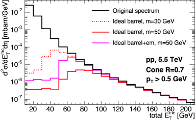
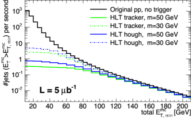
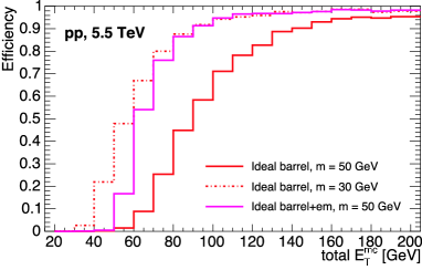
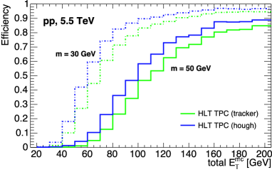
In fig. 22(a) the original input spectrum is compared to the triggered spectrum of jets, depending on different ideal detector cases and values of the required energy in the cone. The shown spectra are normalized to the inclusive single-jet cross section at mid-pseudo-rapidity in pp at $\sqrt{s}=5.5\leavevmode\nobreak\ \mbox{${\rm TeV}$}$. As expected, the cut on the energy in the cone suppresses low energy jets. Since the energy resolution in case of an ideal EMCAL is significantly higher, the choice of $m=50\leavevmode\nobreak\ \mbox{${\rm GeV}$}$ leads to a sharper cut than for the ideal barrel only. This is quantified in fig. 23(a), where the efficiency of the trigger is plotted for the same settings. The efficiency is defined by the fraction of triggered jets to total jets (entering the simulation) as a function of the jet energy, i.e. the ratio of the triggered to the input spectrum in fig. 22(a). Due to the increased resolution induced by the EMCAL, the rise of the efficiency occurs around the value given by $m$, and, furthermore, is relatively steep. In fig. 22(b), we show the rate of triggered jets with $E_{\mathrm{T}}^{\rm mc}>E_{\rm T,\,min}^{\rm mc}$ for the HLT tracking case compared to different values of the required energy. The accepted number of events per second, $N_{\rm acc}$, eq. (7), corresponds to the rate at $E_{\rm T,\,min}^{\rm mc}=0$. For the calculation of the rate it is assumed that jet events enter the system at full L1 production rate (labeled ‘Original pp, no trigger’, i.e. $m=0$, cf. fig. 3). Thus, for pp with the chosen values of $m$, the trigger stays well below an event rate of $10\leavevmode\nobreak\ \mbox{${\rm Hz}$}$, if a value of $m=30\leavevmode\nobreak\ \mbox{${\rm GeV}$}$ is used. Obviously, one could even afford to use a smaller value of $m$. This is opposed to Pb–Pb, see below. The corresponding efficiencies of the two HLT cases are shown in fig. 23(b). In table 3, we report the resulting yearly yields in pp at $\sqrt{s}=5.5\leavevmode\nobreak\ \mbox{${\rm TeV}$}$, compared to rates, one would obtain with the trigger based on the ideal barrel, and compared to the total number of produced jets at L1 (taken from table 1). In addition, we report the total number of accepted events per year. Since there is a lower cut on the jets in the simulation (cf.to the first $p_{\mathrm{T}}^{\rm hard}$-interval), $N_{\rm acc}$ is evaluated at $E_{\rm T,\,min}^{\rm mc}=15\leavevmode\nobreak\ \mbox{${\rm GeV}$}$ and, therefore, not precise. Note that the triggered

Case	Ideal barrel		HLT tracker		HLT hough		Total L1
$m$ [${\rm GeV}$]	$30$	$50$	$30$	$50$	$30$	$50$	$0$
$Y(50\leavevmode\nobreak\ \mbox{${\rm GeV}$})$	$2.3\cdot 10^{7}$	$4.8\cdot 10^{6}$	$1.5\cdot 10^{7}$	$2.8\cdot 10^{6}$	$2.1\cdot 10^{7}$	$4.8\cdot 10^{6}$	$4.9\cdot 10^{7}$
$Y(100\leavevmode\nobreak\ \mbox{${\rm GeV}$})$	$1.6\cdot 10^{6}$	$1.3\cdot 10^{6}$	$1.4\cdot 10^{6}$	$9.6\cdot 10^{5}$	$1.5\cdot 10^{6}$	$1.1\cdot 10^{6}$	$2.2\cdot 10^{6}$
$Y(150\leavevmode\nobreak\ \mbox{${\rm GeV}$})$	$2.4\cdot 10^{5}$	$2.3\cdot 10^{5}$	$1.9\cdot 10^{5}$	$2.3\cdot 10^{5}$	$2.3\cdot 10^{5}$	$2.1\cdot 10^{5}$	$3.0\cdot 10^{5}$
$Y(200\leavevmode\nobreak\ \mbox{${\rm GeV}$})$	$4.2\cdot 10^{4}$	$4.1\cdot 10^{4}$	$4.0\cdot 10^{4}$	$3.7\cdot 10^{4}$	$4.1\cdot 10^{4}$	$3.8\cdot 10^{4}$	$5.4\cdot 10^{4}$
$N_{\rm acc}$	$4.4\cdot 10^{7}$	$5.1\cdot 10^{6}$	$2.6\cdot 10^{7}$	$3.4\cdot 10^{6}$	$4.8\cdot 10^{7}$	$7.3\cdot 10^{6}$	$5.0\cdot 10^{9}$

Table 3: Jet yield per ALICE run year in pp at $\sqrt{s}=5.5\leavevmode\nobreak\ \mbox{${\rm TeV}$}$ corresponding to the rates shown in fig. 22(b) compared to the rates obtained for the ideal barrel and the total produced jets at full L1 rate. $N_{\rm acc}$ is evaluated at $E_{\rm T,\,min}^{\rm mc}=15\leavevmode\nobreak\ \mbox{${\rm GeV}$}$.

Coming to central Pb–Pb collisions, the situation for the trigger changes. We embed the pp spectrum, or rather the corresponding pp events, generated with PYTHIA as mentioned above in $0$–$10$% central HIJING events with settings listed in section 7.C on page 7.C.  In that way, the performance of the trigger algorithm in Pb–Pb can be evaluated as before, since the signal jets may be identified with the bookmarked original jets from PYTHIA. As usual in Pb–Pb, $R=0.3$ and a cut of $p_{\mathrm{T}}>2\leavevmode\nobreak\ \mbox{${\rm GeV}$}$ are used, also for the trigger. Since no realistic detector response is available, different ideal cases are evaluated.

Figure 24(a) shows the trigger rate of signal jets with $E_{\mathrm{T}}^{\rm mc}>E_{\rm T,\,min}^{\rm mc}$ as a function of $E_{\rm T,\,min}^{\rm mc}$ for different choices of $m$. For the calculation of the rates it is assumed that jet events enter the system at full L1 minimum-bias production rate (labeled as ‘PbPb, minimum-bias’, i.e. $m=0$, cf. fig. 3). Note that the background is still approximated by $0$–$10$% HIJING, not adjusted to minimum-bias.  The total number of triggered events per second corresponds to $E_{\rm T,\,min}^{\rm rec}=0$. It is indicated as thin horizontal lines for the different settings and values of $m$. Thus, the trigger for $m=30\leavevmode\nobreak\ \mbox{${\rm GeV}$}$ does not significantly reduce the rate arising from the HIJING background. The reason is that the background itself contains jet signatures and correlations (HIJING quenched), which even with the proposed cone finder settings $R=0.3$ and $p_{\mathrm{T}}>2\leavevmode\nobreak\ \mbox{${\rm GeV}$}$ lead to reconstructed jets of $50\leavevmode\nobreak\ \mbox{${\rm GeV}$}$, and even more. In fig. 24(b) the fraction of accepted background is estimated as a function of $m$ for the ideal cases. In the case of the ideal barrel, for $m=30\leavevmode\nobreak\ \mbox{${\rm GeV}$}$ about every tenth event will trigger, even if no signal is embedded. However, for $m=50\leavevmode\nobreak\ \mbox{${\rm GeV}$}$ this accidental trigger rate is already suppressed by one order of magnitude. In fig. 25(a), the efficiency, defined as the ratio of the number of triggered signal jets to the total number of signal jets, is plotted as a function of $E_{\rm T,\,min}^{\rm mc}$. Figure 25(b) shows the corresponding significance of the trigger, defined as the ratio of the number of triggered signal jets to total number of triggered events.

(a) Trigger rate in minimum-bias Pb–Pb (ideal)

(b) Fraction of accepted background (ideal)

Figure 24: 24(a) Trigger rate of signal jets with $E_{\mathrm{T}}^{\rm mc}>E_{\rm T,\,min}^{\rm mc}$ for ideal cases at different values of the required energy ($m$). The minimum-bias input contains the original pp spectrum embedded into background ($0$–$10$% Pb–Pb, HIJING). The horizontal lines show the total rate of triggered events per second. 24(b) Fraction of accepted events in pure background ($0$–$10$% Pb–Pb, HIJING) for ideal cases as a function of the required energy ($m$). In both figures $R=0.3$ and $p_{\mathrm{T}}\geq 2\leavevmode\nobreak\ \mbox{${\rm GeV}$}$ are used.

(a) Trigger efficiency in central Pb–Pb (ideal)

(b) Significance in central Pb–Pb (ideal)

Figure 25: Trigger efficiency 25(a) and significance 25(b) for ideal cases as a function of the total $E_{\mathrm{T}}$ given by the Monte Carlo jets at different values of the required energy ($m$). The pp spectrum is embedded into background ($0$–$10$% Pb–Pb, HIJING); $R=0.3$ and $p_{\mathrm{T}}\geq 2\leavevmode\nobreak\ \mbox{${\rm GeV}$}$ are used.

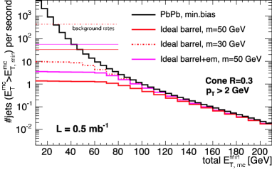
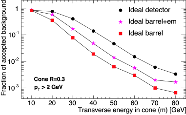
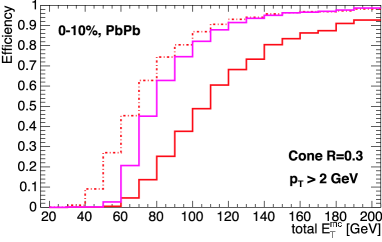
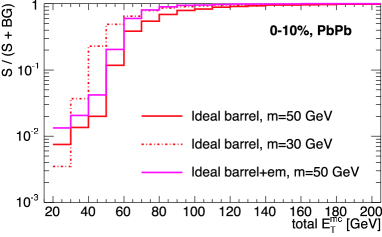
Both figures confirm that, while the lower value of $m$ generally improves the efficiency, it reduces the significance mainly at low jet energies leading to a high number of accepted events. Thus, for Pb–Pb the trigger threshold must be increased to about $m=50\leavevmode\nobreak\ \mbox{${\rm GeV}$}$, in order to acquire event rates, which can be handled by the DAQ system. For $m=50\leavevmode\nobreak\ \mbox{${\rm GeV}$}$, ALICE should preferably run in the barrel+em case, which greatly improves the efficiency and signal-to-noise ratio. Finally, we report the resulting yearly yields in table 4 for minimum-bias Pb–Pb at $\sqrt{s_{\scriptscriptstyle{{\rm NN}}}}=5.5\leavevmode\nobreak\ \mbox{${\rm TeV}$}$ compared to total number of produced jets at full L1 rate (taken from table 1). The corresponding yields for central events may approximately deduced by dividing the minimum-bias yields by a factor of $2.5$. In addition, we report the total accepted number of events per year evaluated at $E_{\rm T,\,min}^{\rm mc}=15\leavevmode\nobreak\ \mbox{${\rm GeV}$}$. 

Case	Ideal barrel		Ideal barrel+em	Total L1
$m$ [${\rm GeV}$]	$30$	$50$	$50$	$0$
$Y(50\leavevmode\nobreak\ \mbox{${\rm GeV}$})$	$6.6\cdot 10^{6}$	$1.3\cdot 10^{6}$	$3.3\cdot 10^{6}$	$2.1\cdot 10^{7}$
$Y(100\leavevmode\nobreak\ \mbox{${\rm GeV}$})$	$6.7\cdot 10^{5}$	$4.7\cdot 10^{5}$	$6.6\cdot 10^{5}$	$9.4\cdot 10^{5}$
$Y(150\leavevmode\nobreak\ \mbox{${\rm GeV}$})$	$9.8\cdot 10^{4}$	$8.9\cdot 10^{4}$	$9.9\cdot 10^{4}$	$1.3\cdot 10^{5}$
$Y(200\leavevmode\nobreak\ \mbox{${\rm GeV}$})$	$1.8\cdot 10^{4}$	$1.7\cdot 10^{4}$	$1.8\cdot 10^{3}$	$2.3\cdot 10^{4}$
$N_{\rm acc}$	$4.4\cdot 10^{8}$	$3.4\cdot 10^{7}$	$5.7\cdot 10^{7}$	$2.1\cdot 10^{9}$

Table 4: Jet yield and total number of triggered events per ALICE run year in minimum-bias Pb–Pb at $\sqrt{s_{\scriptscriptstyle{{\rm NN}}}}=5.5\leavevmode\nobreak\ \mbox{${\rm TeV}$}$ corresponding to the rates shown in fig. 24(a) compared to the production at full L1 rate. $N_{\rm acc}$ is evaluated at $E_{\rm T,\,min}^{\rm mc}=15\leavevmode\nobreak\ \mbox{${\rm GeV}$}$.

In summary, in pp for $m=30\leavevmode\nobreak\ \mbox{${\rm GeV}$}$ and in Pb–Pb for $m=50\leavevmode\nobreak\ \mbox{${\rm GeV}$}$ the rate may be reduced by about a factor of $50$ for Pb–Pb ($100$ for pp), while keeping $1/10$ ($1/5$ for pp) of the events with $E_{\rm T,\,min}^{\rm mc}=50\leavevmode\nobreak\ \mbox{${\rm GeV}$}$ and more than half of the events with $E_{\rm T,\,min}^{\rm mc}=100\leavevmode\nobreak\ \mbox{${\rm GeV}$}$. Running in the case of the ideal barrel will provide enough statistics at high energies. However, one should keep in mind that without an EMCAL a bias towards charged-particle fragmentation will be introduced in the recorded data sample, and —throughout the thesis— full $2\pi$ coverage in $\phi$ is assumed for the EMCAL. Furthermore, without hardware triggering at L1 (neglecting the possibility of the TRD) the yields will drop by about a factor of $350$ in pp and a factor of $4$ in Pb–Pb (see section 2).

5 Expected back-to-back jet rates

It might be useful to estimate the cross section of jet pairs which emerge back-to-back in azimuth in the ALICE central acceptance. Typically one computes the dijet mass spectrum, $\mathrm{d}^{3}\sigma/\mathrm{d}M_{\rm jj}/\mathrm{d}\eta_{1}\mathrm{d}\eta_{2}$, where the dijet mass in the centre-of-mass system is defined according to

$$M_{\rm jj}^{2}=2E_{\mathrm{T}}^{\rm jet1}\,E_{\mathrm{T}}^{\rm jet2}\left(\cosh(\Delta\eta^{\rm 1\,2}_{J})-\cos(\Delta\phi^{\rm 1\,2}_{J})\right)$$

assuming the jets are massless [245]. In our case we are interested in back-to-back jets, where $\Delta\phi^{\rm 1\,2}_{J}\approx\pi$. To compute the corresponding spectrum we generate pairs of jets using PYTHIA in the way described in section 7.B on page 7.B. Since we need to be able to reconstruct both jets (of the dijet) in the central barrel their jet axes must be in the interval of $-0.5<\eta^{\rm jet1}_{J},\,\eta^{\rm jet2}_{J}<0.5$ to be accepted. Furthermore, ensuring that the jets are pointing back-to-back in azimuth we require $\frac{5}{6}\pi\leq\left|\Delta\phi_{J}^{\rm 1\,2}\right|\leq\frac{7}{6}\pi$. In addition, we might apply a restriction to the magnitude of their relative transverse energy

$$E_{\mathrm{T}}^{\rm jet2}\geq f\,E_{\mathrm{T}}^{\rm jet1}\;,$$

where $0\leq f\leq 1$ and $E_{\mathrm{T}}^{\rm jet2}\geq 10\leavevmode\nobreak\ \mbox{${\rm GeV}$}$ assuming $E_{\mathrm{T}}^{\rm jet1}$ is the energy of the leading jet.

Figure 26: Back-to-back jet and direct photon–jet cross sections for $f=0$ and $f=0.9$ at mid-pseudo-rapidity in pp interactions at $5.5\leavevmode\nobreak\ \mbox{${\rm TeV}$}$ simulated with PYTHIA compared to the inclusive single-jet cross section at the same energy. In all cases the jets are identified with the UA1 cone finder for $R=1.0$ using particles in the central ALICE acceptance ($\left|\eta\right|<1$). For further details see the text describing the figure.

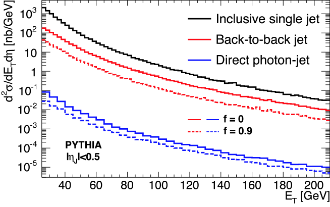
In fig. 26 we report the cross section, $\mathrm{d}^{2}\sigma/\mathrm{d}E_{\mathrm{T}}\,\mathrm{d}\eta$, for jet pairs fulfilling the back-to-back conditions compared to the single-inclusive spectrum. The jets are reconstructed with the UA1 cone finder for $R=1.0$ using particles without detector response in the central ALICE acceptance ($\left|\eta\right|<1$). The single-jet spectrum is the same as shown in fig. 2, but note the change of the scale to nb.  Compared to the single-inclusive the back-to-back jet cross section for $f=0$ is about an order of magnitude smaller at low energies, while for $E_{\mathrm{T}}>100\leavevmode\nobreak\ \mbox{${\rm GeV}$}$ it is about a factor of $5$ smaller. Taking $f=0.9$ dramatically reduces the cross section up to a factor of $50$ at low energies, while at $50\leavevmode\nobreak\ \mbox{${\rm GeV}$}$ the difference is about a factor of $20$ gradually reducing to about difference of a factor of $10$ at highest energies.

For completeness we also show in fig. 26 the direct photon–jet cross section for $f=0$ and $f=0.9$, respectively. Here, the leading jet is replaced by prompt photons (mainly $\mbox{$\mathrm{q}$}\mbox{$\mathrm{\overline{q}}$}\rightarrow\mbox{$\mathrm{g}$}\mbox{$\mathrm{\gamma}$}$ and $\mbox{$\mathrm{q}$}\mbox{$\mathrm{g}$}\rightarrow\mbox{$\mathrm{q}$}\mbox{$\mathrm{\gamma}$}$).  The prompt photon together with reconstructed hadronic jet from the fragmentation of the quark or gluon is required to fulfill the same conditions as above. Due to the electromagnetic origin of the prompt photon the cross section is suppressed by more than three orders of magnitude. We see that the requirement of $f=0.9$ reduces the cross section by an additional factor of about $4$ at low energies to about $2$ at high energies.

Finally in table 5 and table 6 we report the yearly yield obtained at L1 for back-to-back jet and photon–jet production in pp collisions at $\sqrt{s}=5.5\leavevmode\nobreak\ \mbox{${\rm TeV}$}$ and in minimum-bias Pb–Pb collisions at $\sqrt{s_{\scriptscriptstyle{{\rm NN}}}}=5.5\leavevmode\nobreak\ \mbox{${\rm TeV}$}$ according to eq. (4) as explained in section 2. Back-to-back jet or photon–jet correlation might play an important role in the understanding of final partonic state effects in Pb–Pb collisions. However, we see that mainly for the interesting case of photon–jet correlations, where the quark or gluons jet contains almost the same energy as the prompt photon in the ALICE acceptance, we run into the statistical limit at energies beyond $25\leavevmode\nobreak\ \mbox{${\rm GeV}$}$.

Collision type	pp, $5.5\leavevmode\nobreak\ \mbox{${\rm TeV}$}$		Pb–Pb, minimum-bias
Fraction of $E_{\mathrm{T}}$ ($f$)	$0$	$0.9$	$0$	$0.9$
$Y_{\rm L1}^{\rm year}(50\leavevmode\nobreak\ \mbox{${\rm GeV}$})$	$3.8\cdot 10^{6}$	$9.4\cdot 10^{5}$	$1.6\cdot 10^{6}$	$4.1\cdot 10^{5}$
$Y_{\rm L1}^{\rm year}(100\leavevmode\nobreak\ \mbox{${\rm GeV}$})$	$2.3\cdot 10^{5}$	$6.2\cdot 10^{4}$	$9.9\cdot 10^{4}$	$2.7\cdot 10^{4}$
$Y_{\rm L1}^{\rm year}(150\leavevmode\nobreak\ \mbox{${\rm GeV}$})$	$3.6\cdot 10^{4}$	$1.1\cdot 10^{4}$	$1.5\cdot 10^{4}$	$4.6\cdot 10^{3}$
$Y_{\rm L1}^{\rm year}(200\leavevmode\nobreak\ \mbox{${\rm GeV}$})$	$6.7\cdot 10^{3}$	$2.1\cdot 10^{3}$	$2.9\cdot 10^{3}$	$8.9\cdot 10^{3}$

Table 5: Back-to-back jet yield per ALICE run year in pp collisions at $\sqrt{s}=5.5\leavevmode\nobreak\ \mbox{${\rm TeV}$}$ and in minimum-bias Pb–Pb collisions at $\sqrt{s_{\scriptscriptstyle{{\rm NN}}}}=5.5\leavevmode\nobreak\ \mbox{${\rm TeV}$}$, both at full L1 rate.

Collision type	pp, $5.5\leavevmode\nobreak\ \mbox{${\rm TeV}$}$		Pb–Pb, minimum-bias
Fraction of $E_{\mathrm{T}}$ ($f$)	$0$	$0.9$	$0$	$0.9$
$Y_{\rm L1}^{\rm year}(25\leavevmode\nobreak\ \mbox{${\rm GeV}$})$	$1.0\cdot 10^{4}$	$3.6\cdot 10^{3}$	$4.3\cdot 10^{3}$	$1.6\cdot 10^{3}$
$Y_{\rm L1}^{\rm year}(50\leavevmode\nobreak\ \mbox{${\rm GeV}$})$	$1.1\cdot 10^{3}$	$4.8\cdot 10^{2}$	$4.5\cdot 10^{2}$	$2.1\cdot 10^{2}$
$Y_{\rm L1}^{\rm year}(100\leavevmode\nobreak\ \mbox{${\rm GeV}$})$	$8.4\cdot 10^{1}$	$4.5\cdot 10^{1}$	$3.6\cdot 10^{1}$	$2.0\cdot 10^{1}$
$Y_{\rm L1}^{\rm year}(150\leavevmode\nobreak\ \mbox{${\rm GeV}$})$	$1.6\cdot 10^{1}$	$9.0\cdot 10^{0}$	$7.0\cdot 10^{0}$	$4.0\cdot 10^{0}$

Table 6: Direct photon–jet yield per ALICE run year in pp collisions at $\sqrt{s}=5.5\leavevmode\nobreak\ \mbox{${\rm TeV}$}$ and in minimum-bias Pb–Pb collisions at $\sqrt{s_{\scriptscriptstyle{{\rm NN}}}}=5.5\leavevmode\nobreak\ \mbox{${\rm TeV}$}$, both at full L1 rate.

Chapter 5 Jet quenching in ALICE

The preceding discussion has outlined the research interest in jet physics in heavy-ion collisions at the LHC and the potential of the central ALICE detectors for jet identification and reconstruction. Qualitatively, we expect in these collisions hard scattered partons to be used as tomographic probes of the produced partonic matter and, thus, the properties of produced hadronic jets to be modified.

In the present chapter, we will give an outline of the perspectives to study jet modification at LHC conditions. At first, we introduce in section 1 two qualitative regimes of jet energy, where in-medium effects may be studied. In the subsequent sections we discuss the potential for jet-quenching measurements in ALICE, briefly touching the low energy regime in section 2, while focusing in section 3 onto jets accessible only at LHC.

1 Low and high energy regimes

In order to separate qualitative different manifestations of in-medium effects, one may determine on the basis of the measured hadronic final state, whether interaction processes occur in the medium, and, whether they manifest in terms of partonic or hadronic degrees of freedom. Following LABEL:wiedemann2004 we consider a parton of high $E_{\mathrm{T}}$ produced in a hard collision. If the parton escapes into the vacuum, it will reduce its initial virtuality, $Q$, by perturbative parton splitting, until after some time, $\propto 1/Q_{\rm hadr}$, it is degraded to the hadronic scale of about $Q_{\rm hadr}\approx 1\leavevmode\nobreak\ \mbox{${\rm GeV}$}$. Numerical estimates for the time scale of hadronization vary significantly [190, 246], but due to the Lorentz boost to the laboratory frame the scale is proportional to the energy,

$$L_{\rm hadr}\simeq\mathrm{const}/Q_{\rm hadr}^{2}\,E_{\mathrm{T}}\;,$$ (1)

where $\mathrm{const}=2$ to account for multiple parton branching. If instead the hard parton escapes into an infinitely extended QGP, the initial perturbative parton splitting is more efficient because of medium-induced gluon radiation. Since the parton cannot hadronize in the dense medium, after some time its partonic fragments will no longer be distinguished from the heat bath: it is thermalized. To estimate the corresponding time scale, $L_{\rm therm}$, one may require that the hard parton has lost all its energy through medium-induced gluon radiation. According to the BDMPS-Z energy loss formula, eq. (11) on page 11, the partonic thermalization length is given by

$$L_{\rm therm}\simeq\sqrt{4/(\alpha_{\rm S}\,C_{\rm R}\,\hat{q})}\,\sqrt{E_{\mathrm{T}}}\;.$$ (2)

These simplified estimates illustrate that for high $E_{\mathrm{T}}$ perturbative mechanisms may indeed remain undisturbed by hadronization over a significant time scale. Depending on its in-medium path length, $L_{\rm med}$, the hard parton will either be absorbed, $L_{\rm therm}<L_{\rm med}<L_{\rm hadr}$, or it has a sufficiently large transverse energy to suffer only the onset of thermalization processes, $L_{\rm med}<L_{\rm therm}<L_{\rm hadr}$. It is the latter case, in which the parton appears as a medium-modified jet. For lower transverse energies, there is not only a competition between the hadronization and the thermalization mechanism, $L_{\rm hadr}\sim L_{\rm therm}$, but also the possibility that the medium interferes with the dynamics of hadronization, $L_{\rm hadr}\sim L_{\rm med}$.

Taking $\alpha_{\rm S}\,C_{\rm R}=1$ and $\hat{q}=1\leavevmode\nobreak\ \mbox{${\rm GeV}$}^{2}/\mbox{${\rm fm}$}$, the condition $L_{\rm med}<L_{\rm therm}<L_{\rm hadr}$ is fulfilled for partons with $E_{\mathrm{T}}\,{\buildrel>\over{{}_{\sim}}}\,10\leavevmode\nobreak\ \mbox{${\rm GeV}$}$, whereas already at $\hat{q}=5\leavevmode\nobreak\ \mbox{${\rm GeV}$}^{2}/\mbox{${\rm fm}$}$ the conditions requires $E_{\mathrm{T}}\,{\buildrel>\over{{}_{\sim}}}\,20\leavevmode\nobreak\ \mbox{${\rm GeV}$}$ (for $L_{\rm med}=2\leavevmode\nobreak\ \mbox{${\rm fm}$}$). Thus, at LHC opposed to RHIC, for high transverse energies there might be the chance —depending on the concrete value of the transport coefficient— to study the evolution of out-of-equilibrium partons mostly undisturbed by hadronization.

For these jets, the interaction with the medium is expected to manifest in the modification of jet properties deviating from known fragmentation processes in vacuum. Calculations predict that the energy lost by the parton remains inside the jet cone, although redistributed in transverse phase space [247, 155]. The corresponding jet-production cross section is expected to follow binary scaling. However, the jet shape is claimed to broaden and the jet multiplicity to soften and increase [248]. Ideally, one should reconstruct the hadronic energy, which for outstanding high-energy jets may be associated with the energy of the parent parton. For these jets, we will compare differences of known properties to pp and peripheral Pb–Pb collisions. Varying the jet energy, may characterize parton interactions in dense colored matter over the widest possible energy range. These measurements require the full reconstruction power of the central barrel, ideally along with the EMCAL.

2 Inclusive leading-particle and jet-like correlations

We restrict the discussion to low energies, $5\leavevmode\nobreak\ \mbox{${\rm GeV}$}<E_{\mathrm{T}}<30\leavevmode\nobreak\ \mbox{${\rm GeV}$}$, of the jet spectrum in Pb–Pb collisions, where there is some overlap with mini-jet and jet production at ongoing and future RHIC measurements.

The main problem of jet identification in heavy-ion collisions is the complexity of the underlying high-multiplicity background, as we have seen in the previous chapter. At these energies, jets cannot be reconstructed as identified objects, neither at RHIC, nor at LHC. Therefore, in this range one is limited to discerning QCD medium effects from intermediate to high-$p_{\mathrm{T}}$ inclusive spectra and angle or energy correlation studies. This restricts what can be unambiguously learned about jet quenching, since, for example, no primary parton momentum can be deduced.

However, such measurements may provide the best means to directly compare the matter produced at RHIC with that produced at the LHC. As outlined above, the physics issues in the low energy regime, common to both colliders, may be distinctly different from the higher energy regime, uniquely accessible at LHC. It is expected and supported by RHIC measurements that in-medium modifications of the jet structure will be stronger at low jet energies effects. Therefore, it will be interesting to quantify changes in the produced matter from RHIC to LHC.

(a) Particle density (ideal barrel)

(b) Fragmentation estimation (ideal barrel)

Figure 1: 1(a) Particle-density distribution, $(2\pi R)^{-1}\mathrm{d}N/\mathrm{d}R$, for correlated and uncorrelated particles as a function of $R$ obtained with $p_{\mathrm{T}}^{\rm seed}=5\leavevmode\nobreak\ \mbox{${\rm GeV}$}$ and a $p_{\mathrm{T}}$-cut of $3\leavevmode\nobreak\ \mbox{${\rm GeV}$}$ in $0$–$10$% central Pb–Pb collisions. 1(b) Estimation of the fragmentation function of correlated particles compared to the uncorrelated background in $0$–$10$% central Pb–Pb collisions. Both figures are adapted from LABEL:cormier2004.

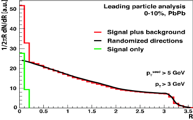
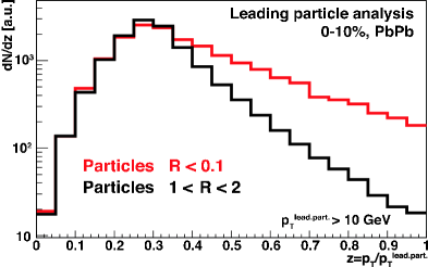
To study correlations with leading particles, an algorithm similar to the one used for the CDF charged-jet analysis is used [250]. Central Pb–Pb collisions are simulated using HIJING as explained in section 7.C on page 7.C. The discussion is limited to the case of the ideal barrel.

All charged particles with $p_{\mathrm{T}}>p_{\mathrm{T}}^{\rm seed}$ are initially regarded as leading-particle candidates, $P_{i}$, ordered according to their transverse momentum, i.e. $P_{0}>P_{1}>\cdots>P_{n}$. The algorithm starts with the highest candidate, $P_{0}$, and records the distances $R$ in the $\eta\times\phi$ space between all particles (above a certain $p_{\mathrm{T}}$-threshold) and $P_{0}$. If another candidate is found within a distance $R<R_{\rm sep}=1.3$ it is eliminated from the list of candidates. The procedure continues with the next candidate on the list until no candidate is left. The algorithm is a natural extension of the cone algorithms (see section 2 on page 2) to be used for inclusive studies in the low jet-energy region for heavy-ions collisions.

To visualize possible angular correlations, one may plot the density, $(2\pi R)^{-1}\mathrm{d}N/\mathrm{d}R$, as a function of the distance, $R$ shown in fig. 1(a). The distribution is obtained for $p_{\mathrm{T}}^{\rm seed}=5\leavevmode\nobreak\ \mbox{${\rm GeV}$}$ with a $p_{\mathrm{T}}$-cut on all particles of $3\leavevmode\nobreak\ \mbox{${\rm GeV}$}$. After subtracting the corresponding distribution for randomized leading-particle directions, a clear near-side correlation signal is visible for $R<0.3$, which results from the mini-jets present in the HIJING simulation

The distribution of the ratio given by the transverse momentum of the correlated particles to the transverse momentum of the leading-particle, $z=p_{\mathrm{T}}/p_{\mathrm{T}}^{\rm lead.part.}$, is an estimator of the jet FF. It is shown in fig. 1(b) for particles in the near-side correlation with $R<0.1$, compared to the background distribution obtained from uncorrelated particles with $1<R<2$. The signal dominates by a large factor at higher $z$-values. The FF approximated by the correlated particles suffers from the fact that the estimation of the jet energy by $p_{\mathrm{T}}^{\rm lead.part.}$ is rather poor, smearing out the true jet FF. However, since in-medium modification of the FF will be strong for low energy jets, it is reasonable to expect that the quenching effect should be observed in the measured leading-particle distribution, for example by comparing central versus peripheral Pb–Pb collisions.

This section limited in scope is based on Refs. [81, 249], where the reader may find further details and observables, which are partially covered in the next section, at high $E_{\mathrm{T}}$.

3 Identified jets at high energy

We will now focus on studies with identified jets for $E_{\mathrm{T}}\,{\buildrel>\over{{}_{\sim}}}\,50\leavevmode\nobreak\ \mbox{${\rm GeV}$}$. In combination with results at lower energies from correlation methods, mentioned above, these measurements might complete the picture of medium-induced parton-energy-loss phenomena. It is our aim to deduce medium effects based merely on the comparison with measurements in pp.

The unquenched spectrum representing the pp reference is generated as in section 4 on page 4, using 10000 PYTHIA events at $\sqrt{s}=5.5\leavevmode\nobreak\ \mbox{${\rm TeV}$}$ per $p_{\mathrm{T}}^{\rm hard}$ interval. Quenched signal jets are simulated in the same way, however, by a modified version of PYTHIA, described in section 7.E on page 7.E. It introduces parton energy loss via final-state gluon radiation, in a rather ad-hoc way: Before the partons originating from the hard $2$-to-$2$ process (and the gluons originating from ISR) are subject to fragment, they are replaced according

$${\rm parton}_{i}(E)\rightarrow{\rm parton_{i}}(E-\Delta E)+n(\Delta E)\,{\rm gluon}(\Delta E/n(\Delta E))$$

conserving energy and momentum. We distinguish between two toy models, where $\Delta E$ and $n(\Delta E)$ are given as follows:

• fixed energy loss: $\Delta E/E=0.2$ and $n=1$ independent of parton type and parton production point in the system (geometry);

• variable energy loss: $\Delta E$ given by PQM for the non-reweighted case, dependent on medium density, parton type and parton production point in the system (geometry). In the following discussion, we will compare jet samples prepared for $k=5\cdot 10^{5}$, $5\cdot 10^{6}$ and $1\cdot 10^{7}\leavevmode\nobreak\ \mbox{${\rm fm}$}$, which for $0$–$10$% central Pb–Pb collisions lead to $\left<\hat{q}\right>=1.2$, $12$ and $24\leavevmode\nobreak\ \mbox{${\rm GeV}$}^{2}/\mbox{${\rm fm}$}$. The choice of the first value implies only a very little modification of the embedded quenched jets compared to the embedding with the standard PYTHIA. The second corresponds to the value of $k$ found to describe the $R_{\rm AA}$ at RHIC, whereas the third is a conservative choice below the extrapolation from RHIC to LHC (in fact, a factor of $5$ lower, see section 4 on page 4). The number of radiated gluons, $1\leq n(\Delta E)\leq 6$, is determined by the condition that each gluon must have less energy than the quenched parton from which it was radiated away. 

The fixed model with the chosen parameters applied to leading-hadron analysis, via eq. (36), would approximately yield $R_{\rm AA}\sim 0.25$ (for $n(p_{\mathrm{T}})\sim 7$), which is comparable to the value obtained by PQM for $\left<\hat{q}\right>=12\leavevmode\nobreak\ \mbox{${\rm GeV}$}^{2}/\mbox{${\rm fm}$}$ (cf. fig. 41 on page 41). Nevertheless, both models are conceptually very different. In the fixed model all initial partons are quenched in the same way regardless of their identity and production point in the collision, i.e. without surface effect. Instead PQM introduces the BDMPS-Z-SW framework and the geometry of the collision, and, thus, partons are treated based on their identity and depending on their path trough the medium. In the latter case, there will be jets, which suffer no or almost no quenching, and jets, which suffer maximum quenching. However, due to the trigger bias, one is predominantly sensitive to jets, emerging close to the surface.

The sample of jets prepared with the modified PYTHIA version is then embedded into $0$–$10$% central HIJING events.  These events represent the quenched spectrum in Pb–Pb and will be discussed in the following. As in the previous section the analysis is mostly restricted to the case of the ideal barrel, i.e. charged particles in the central ALICE acceptance taken from Monte Carlo without simulated detector response. To cope with the soft background in Pb–Pb we use the cone finder, ILCA, with $R=0.3$ and a cut of $p_{\mathrm{T}}>2\leavevmode\nobreak\ \mbox{${\rm GeV}$}$, also for the reference measurement in pp. The number of jets with highest initial energies ($\sim 200\leavevmode\nobreak\ \mbox{${\rm GeV}$}$) in the sample roughly corresponds to the number within the integrated yield of one ALICE year in Pb–Pb ($\sim 10^{4}$), assuming we can fully exploit the maximum L1 jet production rate. For lower jet energies, weights reflecting their increase in cross section are introduced to account for their predominance in the sample. Statistical errors for these events are therefore not representative.

In the following it is our aim to discuss simple, model-independent observables, which might be sensitive to in-medium modification of jets, but insensitive to soft particles from the underlying background event, and to compare the different quenching scenarios.  For the scope of the thesis, the analysis will be restricted to jets with highest energy in the event. We know from the previous chapter that the energy resolution in Pb–Pb in the case of the ideal barrel alone is limited to a mean and width of about $50$%. Therefore, we will introduce for all observables a lower bound on the energy of jets, which are included in the analysis, $E_{\mathrm{T}}^{\rm rec}>E_{\rm T,\,min}^{\rm rec}$. This way it is ensured that the true energy of the jets in the sample cannot be lower than $E_{\rm T,\,min}^{\rm rec}$, however the jets still may contain contributions from the underlying background. Due to the steeply falling jet-production spectrum, the analysis will be dominated by jets, whose true energy leads, on average, to about $E_{\rm T,\,min}^{\rm rec}$.

1 Longitudinal and transverse momentum distributions

The physics signature of medium-induced gluon radiation generally is believed to be visible in the modification of the jet Fragmentation Function (FF) as measured through the longitudinal and transverse momentum distributions of associated hadrons within the jet. The momenta parallel to the jet axis, $p_{\rm L}=p_{\rm hadron}\,\cos(\theta_{\rm jet},\theta_{\rm hadron})$, are expected to be reduced (jet quenching), while the momenta in the transverse direction, $j_{\rm T}=p_{\rm hadron}\,\sin(\theta_{\rm jet},\theta_{\rm hadron})$, to be increased (transverse heating).

(a) Longitudinal for $E_{\mathrm{T}}^{\rm rec}>30\leavevmode\nobreak\ \mbox{${\rm GeV}$}$ (ideal barrel)

(b) Longitudinal for $E_{\mathrm{T}}^{\rm rec}>80\leavevmode\nobreak\ \mbox{${\rm GeV}$}$ (ideal barrel)

Figure 2: Longitudinal momentum distributions, with respect to the jet axis, for charged particles in jets with $E_{\mathrm{T}}^{\rm rec}>30\leavevmode\nobreak\ \mbox{${\rm GeV}$}$ 2(a) and $E_{\mathrm{T}}^{\rm rec}>80\leavevmode\nobreak\ \mbox{${\rm GeV}$}$ 2(b) for different quenching scenarios in $0$–$10$% central Pb–Pb compared to pp collisions. The inset shows the ratio of the distribution for the different Pb–Pb cases to the distribution obtained in pp. In both figures the jets are identified with the ILCA cone finder using $R=0.3$ and $p_{\mathrm{T}}>2\leavevmode\nobreak\ \mbox{${\rm GeV}$}$ in case of the ideal barrel.

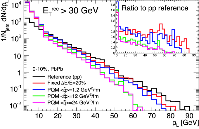
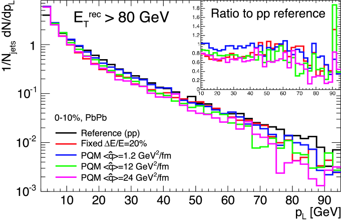
In fig. 2(a) we show the longitudinal distribution for different quenching scenarios in $0$–$10$% central Pb–Pb compared to pp collisions taking into account all reconstructed jets where $E_{\mathrm{T}}^{\rm rec}>30\leavevmode\nobreak\ \mbox{${\rm GeV}$}$. The expected behavior is clearly visible: higher medium density leads to stronger suppression of the momenta along the jet axis and enhancing of smaller momenta. At $p_{\rm L}\,{\buildrel>\over{{}_{\sim}}}\,25\leavevmode\nobreak\ \mbox{${\rm GeV}$}$ the effect of the medium-induce radiation becomes apparent for the two dense PQM cases. However, at low $p_{\rm L}\,{\buildrel<\over{{}_{\sim}}}\,10\leavevmode\nobreak\ \mbox{${\rm GeV}$}$, the strong change of the longitudinal distribution is predominantly induced by the remaining hadrons of the underlying background, since in this region all quenched case agree. It is obvious that jet quenching effects will be measurable in the ratio of the longitudinal distribution obtained for jets in Pb–Pb with respect to pp. However, given the statistics we have at hand, the quantitative distinction between, for example, the two dense PQM scenarios seems to be impossible.

(a) Transverse for $E_{\mathrm{T}}^{\rm rec}>30\leavevmode\nobreak\ \mbox{${\rm GeV}$}$ (ideal barrel)

(b) Transverse for $E_{\mathrm{T}}^{\rm rec}>80\leavevmode\nobreak\ \mbox{${\rm GeV}$}$ (ideal barrel)

Figure 3: Transverse momentum distributions, with respect to the jet axis, for charged particles in jets with $E_{\mathrm{T}}^{\rm rec}>30\leavevmode\nobreak\ \mbox{${\rm GeV}$}$ 2(a) and $E_{\mathrm{T}}^{\rm rec}>80\leavevmode\nobreak\ \mbox{${\rm GeV}$}$ 2(b) for different quenching scenarios in $0$–$10$% central Pb–Pb compared to pp collisions. In both figures the jets are identified with the ILCA cone finder using $R=0.3$ and $p_{\mathrm{T}}>2\leavevmode\nobreak\ \mbox{${\rm GeV}$}$ in case of the ideal barrel.

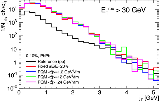
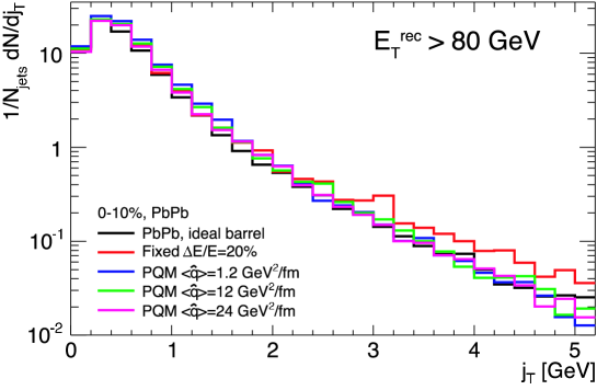
To reduce the contribution of the background, we increase the cut on the jet energy to $E_{\mathrm{T}}^{\rm rec}>80\leavevmode\nobreak\ \mbox{${\rm GeV}$}$ as shown in fig. 2(b). For low momenta the shape of the quenched distributions now turn out to be quite similar to the pp reference. Measuring the excess of low $p_{\rm L}$ with respect to pp will be challenging, but of main interest for the comparison with theory. Looking at the ratio of the Pb–Pb cases with respect to the pp reference, the difference in the strength of the medium-induced radiation becomes seemingly apparent for the two dense cases of PQM, and, by eye, both may be distinguished. Although, for quantitative studies, high statistics will be needed at higher $p_{L}$. For jets, merely reconstructed with the ideal barrel, energies of $E_{\mathrm{T}}^{\rm rec}>80\leavevmode\nobreak\ \mbox{${\rm GeV}$}$ might be at the statistical limit, since the jets, which contribute to the analysis, mainly arise from jets with true energies of about $E_{\mathrm{T}}\,{\buildrel>\over{{}_{\sim}}}\,120\leavevmode\nobreak\ \mbox{${\rm GeV}$}$. As a consequence of the trigger bias and due to the surface effect, a considerable fraction of jets does not (or almost not) suffer from the quenching. This is opposed to the fixed-energy loss model, where jets from all depths are equally quenched. It, therefore, will be fruitful to study the dependence of the $p_{\rm L}$ distribution with collision centrality and —if statistics allows— with respect of the jet direction to the reaction plane.

The momentum distribution transverse to the jet axis is plotted in fig. 3(a) for $E_{\mathrm{T}}^{\rm rec}>30\leavevmode\nobreak\ \mbox{${\rm GeV}$}$. Strong broadening of the transverse distribution compared to the vacuum case is observed. However, the observed modification originates from the mixing with the HIJING event rather from the interactions of the primary parton with the dense medium, since the modified PYTHIA version does not include such effects.  This is confirmed by fig. 3(b) where in the analysis only jets with $E_{\mathrm{T}}^{\rm rec}>80\leavevmode\nobreak\ \mbox{${\rm GeV}$}$ are contributing. Since all models agree with the pp reference, it seems possible that one can exclusively measure transverse broadening for these jets, if it exists in nature.

Since the $j_{\rm T}$ distribution is expected to significantly broaden in central Pb–Pb collisions [248], and since its average has been measured in numerous collider experiments and found to be relatively insensitive to the collision energy [253], the average particle-momentum associated in a jet transverse to the jet axis, $\left<j_{\rm T}\right>$, might be a key observable at the LHC. For our toy models we find $\left<j_{\rm T}\right>=0.7\leavevmode\nobreak\ \mbox{${\rm GeV}$}$ for $E_{\mathrm{T}}^{\rm rec}>30\leavevmode\nobreak\ \mbox{${\rm GeV}$}$ and $\left<j_{\rm T}\right>=0.63\leavevmode\nobreak\ \mbox{${\rm GeV}$}$ for $E_{\mathrm{T}}^{\rm rec}>80\leavevmode\nobreak\ \mbox{${\rm GeV}$}$ compared to $\left<j_{\rm T}\right>=0.51\leavevmode\nobreak\ \mbox{${\rm GeV}$}$ and $\left<j_{\rm T}\right>=0.61\leavevmode\nobreak\ \mbox{${\rm GeV}$}$ in the vacuum. 

It will be interesting to study $\left<j_{\rm T}\right>$ as a function of the minimum jet energy, $E_{\mathrm{T}}^{\rm rec}>E_{\rm T,\,min}^{\rm rec}$, and to link the observed distributions in reconstructed jets with those deduced for jets in the low energy range from correlations studies of leading particles, also for varying centrality.

2 Leading-particle fragmentation

The modification of the jet FF must be reflected in the quenching of the leading-particle transverse momentum, because prior to hadronization the primary parton has lost a considerable fraction of its energy into gluon radiation while traversing the dense medium.  Since it is expected that the radiated gluons will subsequently fragment into hadrons inside the jet cone, the total energy of the jet and its spatial distribution are only moderately modified. It has been shown [248] that the medium-induced broadening of the jet reduces the energy inside $R=0.3$ by $\sim 15$% and by $\sim 7$% for jets with $E_{\mathrm{T}}=50$ and $E_{\mathrm{T}}=100\leavevmode\nobreak\ \mbox{${\rm GeV}$}$, respectively, and already at $R=0.7$ the effect reduces to about $2$%. However, one must be cautious about these findings, since this prediction has been calculated assuming a rather low value of the gluon density at LHC conditions. Furthermore, the calculation has merely been performed at the parton level.

Nevertheless, assuming the energy remains within the cone and assuming that the estimation of $E_{\mathrm{T}}$ with the reconstructed (charged) energy in the reduced size of the cone is accurate enough to not completely mask the effect, the fraction $z=p_{\mathrm{T}}^{\rm lead.part.}/E_{\mathrm{T}}$ might be sensitive to the in-medium modification of the jet FF.

(a) Leading-particle frag. (ideal barrel)

(b) Fraction for $E_{\mathrm{T}}^{\rm rec}>E_{\rm T,\,min}^{\rm rec}$ (ideal barrel)

(c) Leading-particle frag. (ideal barrel+em)

(d) Fraction for $E_{\mathrm{T}}^{\rm rec}>E_{\rm T,\,min}^{\rm rec}$ (ideal barrel+em)

Figure 4: Leading-particle fragmentation in jets with $E_{\mathrm{T}}^{\rm rec}>50\leavevmode\nobreak\ \mbox{${\rm GeV}$}$ in the case of the ideal barrel 4(a) and of ideal barrel+em 4(c) for different quenching scenarios in $0$–$10$% central Pb–Pb compared to pp collisions. Fraction of jet energy carried by the leading particles in jets with $E_{\mathrm{T}}^{\rm rec}>E^{\rm rec}_{\rm T,\,min}$ as a function of $E^{\rm rec}_{\rm T,\,min}$ in the case of the ideal barrel 4(b) and of ideal barrel+em 4(d) for different quenching scenarios in $0$–$10$% central Pb–Pb compared to pp collisions. In all figures the jets are identified with the ILCA cone finder using $R=0.3$ and $p_{\mathrm{T}}>2\leavevmode\nobreak\ \mbox{${\rm GeV}$}$.

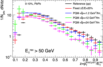
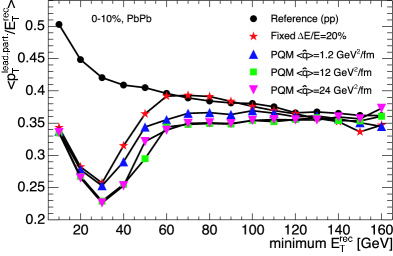
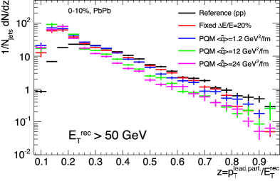
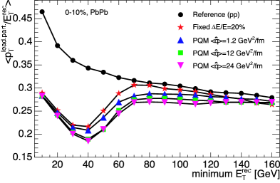
Figure 4(a) shows the fragmentation function for leading particles, $\mathrm{d}N/\mathrm{d}z$ for $z=p_{\mathrm{T}}^{\rm lead.part.}/E_{\mathrm{T}}^{\rm rec}$, in jets where $E_{\mathrm{T}}^{\rm rec}>50\leavevmode\nobreak\ \mbox{${\rm GeV}$}$. Indeed, the expected behavior is visible, higher medium density leads to stronger suppression of the leading particles, mainly at large values of $z$. However, there is the indication of a contribution by the background, at low $z$, shifting the mean of distribution to the left. As before, we can study the artificial contribution of the heavy-ion background by variation of $E^{\rm rec}_{\rm T,\,min}$.

In vacuum the average fraction of the jet energy carried by the leading particle is known, $\left<z\right>\simeq 0.3$ for $E_{\mathrm{T}}\,{\buildrel>\over{{}_{\sim}}}\,100\leavevmode\nobreak\ \mbox{${\rm GeV}$}$ (for $R=0.7$ and $p_{\mathrm{T}}>0.5\leavevmode\nobreak\ \mbox{${\rm GeV}$}$, see section 5 on page 5). Since the average value most likely will change according to the modification of the distribution, we compute $\left<z\right>$ for jets with $E_{\mathrm{T}}^{\rm rec}>E^{\rm rec}_{\rm T,\,min}$ as a function of $E^{\rm rec}_{\rm T,\,min}$ shown in fig. 4(b). At low $E^{\rm rec}_{\rm T,\,min}\,{\buildrel<\over{{}_{\sim}}}\,50\leavevmode\nobreak\ \mbox{${\rm GeV}$}$ all quenching models agree and differ strongly from the reference measurement. In this region, the value of $\left<z\right>$ is determined by properties of the background, resulting in artificial jets, whose leading particle does not arise from jet fragmentation. Instead, at high $E^{\rm rec}_{\rm T,\,min}$ the reconstructed jets are biased to extreme fragmentation and $\left<z\right>$ reaches the magnitude of the pp reference. However, there is indication that within $50\leavevmode\nobreak\ \mbox{${\rm GeV}$}<E^{\rm rec}_{\rm T,\,min}<100\leavevmode\nobreak\ \mbox{${\rm GeV}$}$ different toy models may be discriminated by the different values of $\left<z\right>$, but the effect is smeared by the poor energy resolution. The situation slightly improves, when the information of the EMCAL is added. The fragmentation of leading particles for $E^{\rm rec}_{\rm T,\,min}\,{\buildrel<\over{{}_{\sim}}}\,50\leavevmode\nobreak\ \mbox{${\rm GeV}$}$ in the case of the ideal barrel+em is shown in fig. 4(c) and $\left<z\right>$ as a function of $E^{\rm rec}_{\rm T,\,min}$ in fig. 4(d). Due the improved energy resolution and to the increase in statistics for higher $E_{\mathrm{T}}^{\rm rec}$ different models may, by eye, be distinguished with only little influence of the background over the range of $60\leavevmode\nobreak\ \mbox{${\rm GeV}$}<E^{\rm rec}_{\rm T,\,min}<120\leavevmode\nobreak\ \mbox{${\rm GeV}$}$. Again, the two dense PQM scenarios cannot be distinguished.

As for the longitudinal and transverse fragmentation it will be interesting to study the dependence of the leading-particle fragmentation and its average on centrality and jet direction with respect to the event plane. Generally, one might prefer to avoid normalizing by the reconstructed jet energy, since it introduces various additional biases. Instead, one could analyze the raw $p_{\mathrm{T}}$ distribution for leading particles, in the same way as done above for all associated particles in the jet.

3 Particle multiplicity and momentum

The modifications of the jet FF we discussed so far are connected to the expectation that due to the medium-induced gluon radiation, many rather, soft hadrons are produced in the fragmentation of the primary parton. Therefore, related and simple observables are the average number of particles in the cone and their average transverse momentum.

(a) Average number (ideal barrel)

(b) Average particle-$p_{\mathrm{T}}$ (ideal barrel)

(c) Average number (ideal barrel+em)

(d) Average particle-$p_{\mathrm{T}}$ (ideal barrel+em)

Figure 5: Average number of particles (left) and mean particle-$p_{\mathrm{T}}$ (right) in jets with $E_{\mathrm{T}}^{\rm rec}>E^{\rm rec}_{\rm T,\,min}$ as a function of $E^{\rm rec}_{\rm T,\,min}$ in the case of the ideal barrel (top) and ideal barrel+em (bottom) for different quenching scenarios in $0$–$10$% central Pb–Pb compared to pp collisions. In all figures the jets are identified with the ILCA cone finder using $R=0.3$ and $p_{\mathrm{T}}>2\leavevmode\nobreak\ \mbox{${\rm GeV}$}$.

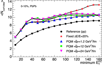
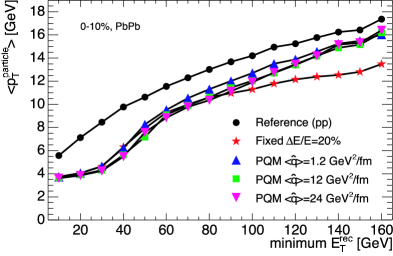
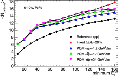
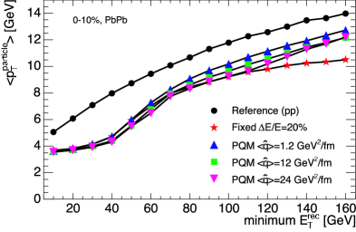
Both are shown in fig. 5 in jets with $E_{\mathrm{T}}^{\rm rec}>E^{\rm rec}_{\rm T,\,min}$ as a function of $E^{\rm rec}_{\rm T,\,min}$ compared for the case of the ideal barrel and the ideal barrel+em. The general picture is as before: at low $E^{\rm rec}_{\rm T,\,min}$ the background masks the difference in the toy models, whereas starting from about $E^{\rm rec}_{\rm T,\,min}\,{\buildrel>\over{{}_{\sim}}}\,50\leavevmode\nobreak\ \mbox{${\rm GeV}$}$ the properties of the identified jets and their different quenching histories may be distinguished. The effect is clearest seen when the $E_{\mathrm{T}}$-resolution is improved by the EMCAL, however using only the charged barrel provides enough information to separate the fixed quenching scenario from the PQM cases. As indicated already in previous plots, the fixed-loss model strongly deviates at high $E^{\rm rec}_{\rm T,\,min}$ from the other models.

4 Integrated jet shapes

Since it is expected that jet quenching leaves a negligible signature in the integrated, calorimetric energy content, it will be important to measure a change in the contribution of soft hadrons to the integrated shape.

(a) $\psi(r)$ for $E_{\mathrm{T}}^{\rm rec}>80\leavevmode\nobreak\ \mbox{${\rm GeV}$}$ (ideal barrel)

(b) $\psi(0.3)$ for $E_{\mathrm{T}}^{\rm rec}>E_{\rm T,\,min}^{\rm rec}$ (ideal barrel)

Figure 6: 6(a) Integrated jet shapes, $\psi(r)$ and $\psi(r)$ where $p_{\mathrm{T}}\leq 5\leavevmode\nobreak\ \mbox{${\rm GeV}$}$, both normalized at $r=1$, of jets with $E_{\mathrm{T}}^{\rm rec}>80\leavevmode\nobreak\ \mbox{${\rm GeV}$}$ for different quenching scenarios in $0$–$10$% central Pb–Pb compared to pp collisions. 6(b) Integrated jet shape $\psi(0.3)$ where $p_{\mathrm{T}}\leq 5\leavevmode\nobreak\ \mbox{${\rm GeV}$}$, normalized at $r=1$, for jets with $E_{\mathrm{T}}^{\rm rec}>E^{\rm rec}_{\rm T,\,min}$ as a function of $E^{\rm rec}_{\rm T,\,min}$ for different quenching scenarios in $0$–$10$% central Pb–Pb compared to pp collisions. In both figures the jets are identified with the ILCA cone finder using $R=0.3$ and $p_{\mathrm{T}}>2\leavevmode\nobreak\ \mbox{${\rm GeV}$}$ in the ideal barrel.

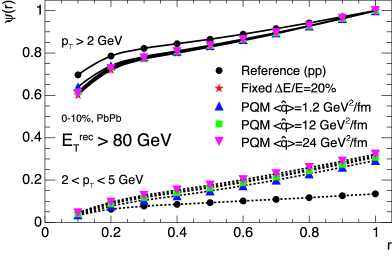
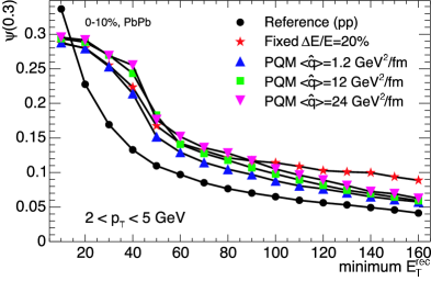
In fig. 6(a) we show the integrated jet shapes, $\psi(r)$, and $\psi(r)$ for particles with $p_{\mathrm{T}}\leq 5\leavevmode\nobreak\ \mbox{${\rm GeV}$}$, in jets with $E_{\mathrm{T}}^{\rm rec}>80\leavevmode\nobreak\ \mbox{${\rm GeV}$}$ as a function of $r$. The jets have been defined only for $R=0.3$, however, we still normalize at $r=1$. A significant fraction of the shape arises due to the soft background, which —mainly at large $r$— stimulates a contribution of soft particles seen, for example, in the linear rise of the shape for particles with $p_{\mathrm{T}}\leq 5\leavevmode\nobreak\ \mbox{${\rm GeV}$}$. Obviously, corrections could be applied. For example, one may substract the contribution of the background evaluated for random jet axis before normalizing the shape at $r=1$ (or at $r\,{\buildrel>\over{{}_{\sim}}}\,0.3$). Once the contribution of the background is under control it will be interesting to compare the shapes measured in Pb–Pb to the measured values in the vacuum, i.e. in the same way as in fig. 13 on page 13.

For the moment, we do not apply any correction, but rather evaluate the shape at fixed $r_{0}=0.3$, the value for which the jets are defined. In fig. 6(b) $\psi(0.3)$ is shown restricted to soft particles with $p_{\mathrm{T}}\leq 5\leavevmode\nobreak\ \mbox{${\rm GeV}$}$ for jets with $E_{\mathrm{T}}^{\rm rec}>E^{\rm rec}_{\rm T,\,min}$ as a function of $E^{\rm rec}_{\rm T,\,min}$. The picture is the same as before: Below $E^{\rm rec}_{\rm T,\,min}=50\leavevmode\nobreak\ \mbox{${\rm GeV}$}$ the contribution of soft particles in the background contributes, for higher values of $E^{\rm rec}_{\rm T,\,min}$, the toy models lead to slightly different values of the shape, and reconcile at highest values of $E^{\rm rec}_{\rm T,\,min}$. In correspondance with the findings above, the fixed energy-loss model deviates from the PQM models.

Chapter 6 Summary

In this work, we study the performance of the ALICE detector for the measurement of high-energy jets at mid-rapidity in ultra-relativistic nucleus–nucleus collisions at $\sqrt{s_{\scriptscriptstyle{{\rm NN}}}}=5.5\leavevmode\nobreak\ \mbox{${\rm TeV}$}$ and their potential for the characterization of the partonic matter created in these collisions.

In our approach, jets at $E^{\mathrm{jet}}_{\mathrm{T}}\,{\buildrel>\over{{}_{\sim}}}\,30\leavevmode\nobreak\ \mbox{${\rm GeV}$}$ are reconstructed with a cone jet finder, as typically done for jet measurements in hadronic collisions. However, the presence of numerous mini-jets in the heavy-ion environment makes it necessary to reduce the cone size, the radius in the plane spanned by pseudo-rapidity and azimuth, from its nominal value of $R\sim 0.7$ used at hadron colliders to $R=0.3$. In addition, the high-particle multiplicity density of the soft bulk at mid-rapidity requires the introduction of a cut in transverse momentum for charged hadrons with $p_{\mathrm{T}}<2\leavevmode\nobreak\ \mbox{${\rm GeV}$}$.

In central lead–lead (Pb–Pb) collisions, jets of about $50\leavevmode\nobreak\ \mbox{${\rm GeV}$}$ and higher will be measurable with ALICE, but intrinsic fluctuations in the jet fragmentation, out-of-cone fluctuations and the remaining underlying mini-jet background limit the energy resolution. This is even valid for an ideal detector and for jets with far higher energy. Without the EMCAL, the resolution is mainly dominated by intrinsic fluctuations in the ratio of charged-to-neutral particles in the jet fragmentation. The mean reconstructed fraction amounts to $50$% (and a width of about $50$%). Including the EMCAL, the mean fraction increases to about $60$% (and a width of $30$%). In both cases, however, the spatial direction of the jet axis can be reconstructed with a resolution (in $\eta$ and $\phi$) of better than $0.01$, at $50\leavevmode\nobreak\ \mbox{${\rm GeV}$}$, which is enough for matching with the direction of the initial parton. The contribution of the background to the energy content within the reduced cone is sizeable, about $15\%$ for $50\leavevmode\nobreak\ \mbox{${\rm GeV}$}$, even with the proposed cuts.

It will be increasingly difficult to resolve the signal from the background for energies lower than $\sim 50\leavevmode\nobreak\ \mbox{${\rm GeV}$}$. In this regime, where jet rates are considerably large, inclusive measurements will be applied. The jet rate in minimum-bias Pb–Pb for jets produced within the central ALICE acceptance drops from one jet per event with $E^{\mathrm{jet}}_{\mathrm{T}}\geq 20\leavevmode\nobreak\ \mbox{${\rm GeV}$}$ to about one jet per $1000$ events with $E^{\mathrm{jet}}_{\mathrm{T}}\geq 100\leavevmode\nobreak\ \mbox{${\rm GeV}$}$. Therefore, for jets with more that $50\leavevmode\nobreak\ \mbox{${\rm GeV}$}$ triggering becomes relevant.

A jet finder running online in the High-Level Trigger (HLT) —using the same algorithm and parameters as for the offline analysis, which is within the time budget— will suppress the recorded data rate by a factor of $50$ for minimum-bias Pb–Pb collisions, while keeping $1/10$ of the jets with $E^{\mathrm{jet}}_{\mathrm{T}}\geq 50\leavevmode\nobreak\ \mbox{${\rm GeV}$}$ and $1/2$ with $E^{\mathrm{jet}}_{\mathrm{T}}\geq 100\leavevmode\nobreak\ \mbox{${\rm GeV}$}$. Even if the HLT system inspects minimum-bias Pb–Pb events without further help of hardware triggers at L1, in total $10^{7}$ events will be recorded in one ALICE year at ${\cal{L}}=0.5\,\mbox{${\rm mb}$}^{-1}\mbox{${\rm s}$}^{-1}$, containing about $4\cdot 10^{5}$ jets with $E^{\mathrm{jet}}_{\mathrm{T}}\geq 50\leavevmode\nobreak\ \mbox{${\rm GeV}$}$ and about $10^{5}$ with $E^{\mathrm{jet}}_{\mathrm{T}}\geq 100\leavevmode\nobreak\ \mbox{${\rm GeV}$}$. The HLT system without further help by hardware triggers is able to provide the necessary statistics. However, for minimization of the trigger bias and for increase in statistics (even if moderate), the HLT should be supported by hardware triggers at L1, as for example foreseen by the EMCAL.

For the study of the sensitivity of high-energy jets to in-medium effects, quenched jets are embedded into central Pb–Pb collisions at $\sqrt{s_{\scriptscriptstyle{{\rm NN}}}}=5.5\leavevmode\nobreak\ \mbox{${\rm TeV}$}$. The jets are prepared for medium densities of $\left<\hat{q}\right>=1.2$, $12$ and $24\leavevmode\nobreak\ \mbox{${\rm GeV}$}^{2}/\mbox{${\rm fm}$}$ using a modified PYTHIA version, which includes partonic energy loss in the BDMPS-Z-SW framework together with a realistic description of the collision geometry.

Our analysis addresses the high-energy regime, where jets may be reconstructed as distinct objects, $E^{\mathrm{jet}}_{\mathrm{T}}\geq 50\leavevmode\nobreak\ \mbox{${\rm GeV}$}$. Still, the comparison with the pp reference reveals that the contamination of the jet cone by uncorrelated particles from the underlying background may severely influence measured jet properties, even up to jet energies of $100\leavevmode\nobreak\ \mbox{${\rm GeV}$}$. Since low-energy jets are predominantly produced, properties of the background mask and, even worse, partially mimic the effect of the medium. However, with increasing energy threshold for the reconstructed jets in the analysis, the influence of the background reduces and most observables show moderate sensitivity, at least.

Even within the limited approach of the quenching procedure, there are a few observables that deserve to be mentioned explicitly. The longitudinal particle-momentum distribution of associated particles along the jet axis is strongly suppressed, measurable for $p_{\rm L}\,{\buildrel>\over{{}_{\sim}}}\,15\leavevmode\nobreak\ \mbox{${\rm GeV}$}$, for example, in the ratio with respect to the measurement in pp. The distribution of the fraction of energy that the leading particle carries changes with respect to the reference. It is shifted towards smaller values, and suppressed at intermediate to high values, $z\,{\buildrel>\over{{}_{\sim}}}\,0.5$. Both distributions have in common that they rely on high-transverse-momentum particles, which are comparatively rare in the underlying background. Instead, the integrated jet shape, by construction, suffers from the soft contribution it receives, since it accounts for all particles in the cone, smearing out the effect of the medium.

The measurement in the charged-particle sector together with the increase of the jet energy threshold proves sufficient to distinguish between the case of lowest and highest medium density. Thus, based on our quenching studies, the detection of in-medium modification in the fragmentation of high-energy jets seems to be possible with the charged-particle tracking detectors, alone.

A word on the quenching procedure seems to be appropriate. Because of the reasoning behind the modified PYTHIA version, relative energy losses of more than $80$% induce the emission of six additional radiated gluons, which share the lost energy of the initial parton at equal parts. Owing to the surface effect, present for both dense cases of the medium, modified jets appear almost similar. Thus, ‘what we see is what we put in’. The limited sensitivity expresses the conceptual difficulties and the lack of theoretical predictiveness within the toy model and, in general, within the BDMPS-Z-SW framework at finite parton energies and for high medium densities. A consistent treatment of medium-induced gluon radiation and the impact on hadronic properties probably requires a Monte Carlo implementation of the medium-modified parton shower.

According to the PQM calculation, high-energy jets with $E^{\mathrm{jet}}_{\mathrm{T}}\,{\buildrel>\over{{}_{\sim}}}\,150\leavevmode\nobreak\ \mbox{${\rm GeV}$}$ might be almost extinct at the LHC. In this case, jet quenching will presumably be detected by calorimetry via apparent reduction of cross section, similar to leading-hadron spectroscopy. ALICE including the EMCAL would be well prepared for such a scenario, too.

Chapter 7 Appendix

Appendix 7.A Glauber calculation

In the following we summarize the essential features of the Glauber formalism [9, 10, 254, 176], which we use in PQM and for the estimations of $N_{\rm coll}$ and $N_{\rm hard}$. The values, which we use throughout the thesis, can be found  tab. 1 on page 1.

Thickness function

The nuclear density profile for a nucleus A in the transverse plane, perpendicular to the beam axis $z$,

$$T_{\rm A}(\vec{s})=\int\mathrm{d}z\,\rho_{\rm A}(z,\vec{s})\;,$$ (1)

is known as the nuclear thickness function of nucleus A. We use the Wood-Saxon nuclear density $\rho_{\rm A}\equiv\rho_{\rm A}^{\rm WS}(z,\vec{r})$ and renormalize $\int\mathrm{d}\vec{s}\,T_{\rm A}(\vec{s})=A$. The parameters of the Wood-Saxon profile for the different nuclei, i.e. gold and lead, can be found in [200].

Overlap function

For a collision of nucleus A with nucleus B the nuclear overlap function, $T_{\rm AB}(\vec{b})$, at impact parameter $\vec{b}$ is defined as

$$T_{\rm AB}(\vec{b})=\int\mathrm{d}\vec{s}\,T_{\rm A}(\vec{s})T_{\rm B}(\vec{b}-\vec{s})\;.$$ (2)

Due to the azimuthal symmetry of the Wood-Saxon profile the integration is conveniently performed using $\mathrm{d}\vec{s}=2\pi\,s\mathrm{d}s$; yielding $A\,B$ for the integral over all impact parameters.

Cross section

In the multiple-scattering approximation of the Glauber formalism the inclusive, inelastic cross-section, $\sigma_{\rm AB},$ for the collision of A and B can be derived, leading to

$$\sigma_{\rm AB}=\int\mathrm{d}\vec{b}\,\left[1-\exp\left(-\sigma_{\rm NN}\,T_{\rm AB}(\vec{b})\right)\right]\;,$$ (3)

where $\sigma_{\rm NN}$ denotes the nucleon–nucleon cross section. We assume that the interaction probability is solely given by the pp cross section. At RHIC $\sigma_{\rm NN}=40\leavevmode\nobreak\ \mbox{${\rm mb}$}$ is usually used. At LHC expectations vary; we use $59\leavevmode\nobreak\ \mbox{${\rm mb}$}$ ($67\leavevmode\nobreak\ \mbox{${\rm mb}$}$), which corresponds to the expected inelastic, but non-diffractive cross section for $\sqrt{s}=5.5\leavevmode\nobreak\ \mbox{${\rm TeV}$}$ ($14\leavevmode\nobreak\ \mbox{${\rm TeV}$}$) [79]. Using eq. (3) gives the total (geometrical) cross section of $\sigma^{\rm geo}_{\rm PbPb}=7.8\leavevmode\nobreak\ \mbox{${\rm b}$}$. Even though, eq. (3) describes a total cross section, to first order it also determines the cross section of a single hard process,

$$\sigma^{\rm hard}_{\rm AB}\approx\int\mathrm{d}\vec{b}\,\sigma^{\rm hard}_{\rm NN}\,T_{\rm AB}(\vec{b})\;,$$ (4)

where $\sigma_{\rm NN}^{\rm hard}\ll\sigma_{\rm NN}$ is the cross section of the hard process in NN interactions.

Binary collisions

For a given impact parameter the average hard scattering yield can be obtained by integrating the probability of the occurrence of an hard process in the interaction of a nucleon of one nucleus multiplied with the interaction probability along its straight trajectory (in $z$) within the other nucleus,

$$N^{\rm hard}_{\rm AB}(b)=\sigma^{\rm hard}_{\rm NN}\int\rho_{\rm A}(z^{\prime},\vec{s})\,\rho_{\rm B}(z^{\prime\prime},\vec{b}-\vec{s})\,\mathrm{d}\vec{s}\,\mathrm{d}z^{\prime}\,\mathrm{d}z^{\prime\prime}=\sigma^{\rm hard}_{\rm NN}\,T_{\rm AB}(\vec{b})\;.$$ (5)

In the same way, one obtains the average number of inelastic, binary NN collisions,

$$N^{\rm coll}_{\rm AB}(b)=\sigma_{\rm NN}\,T_{\rm AB}(\vec{b})\;.$$ (6)

Yields in centrality classes

The above formulas are valid at a given impact parameter. The fraction of the (geometrical) cross section for the centrality selection $C_{1}$–$C_{2}$, corresponding to the impact parameter range $b_{1}<b<b_{2}$, is given by

$$f^{\rm geo}_{\rm AB}(b_{1},b_{2})=\int_{b_{1}<b<b_{2}}\mathrm{d}\vec{b}\,P(\vec{b})$$ (7)

where the probability distribution of impact parameters reads

$$P(\vec{b})=\left[1-\exp\left(-\sigma_{\rm NN}\,T_{\rm AB}(\vec{b})\right)\right]\,/\,\sigma^{\rm geo}_{\rm AB}\;.$$ (8)

For the calculation of the yields in the centrality class, $C_{1}$–$C_{2}$, one needs to take into account the conditional probability that a collision in the given centrality range takes place. For the average nuclear overlap function in the given centrality class we obtain

$$\left<T_{\rm AB}\right>(b_{1},b_{2})=\int_{b_{1}<b<b_{2}}\mathrm{d}\vec{b}\,P(\vec{b})\,T_{\rm AB}(\vec{b})\,/\,f^{\rm geo}_{\rm AB}(b_{1},b_{2})\;.$$ (9)

Using eq. (5) and eq. (6) leads to the yields,

$$\left<N^{\rm hard}_{\rm AB}\right>(b_{1},b_{2})=\left<T_{\rm AB}\right>(b_{1},b_{2})\,\sigma^{\rm hard}_{\rm NN}$$ (10)

for the average number of hard processes and

$$\left<N^{\rm coll}_{\rm AB}\right>(b_{1},b_{2})=\left<T_{\rm AB}\right>(b_{1},b_{2})\,\sigma_{\rm NN}$$ (11)

for the average number of binary NN interactions in the selected centrality range.

Binary scaling

From the last two equations we get binary collision scaling of hard processes according

$$\left<N^{\rm hard}_{\rm AB}\right>(b_{1},b_{2})=\left<N^{\rm coll}_{\rm AB}\right>(b_{1},b_{2})\,\sigma^{\rm hard}_{\rm NN}/\sigma_{\rm NN}$$ (12)

and using eq. (4) with eq. (9) we find for the cross section

$$\sigma^{\rm hard}_{\rm AB}(b_{1},b_{2})=\left<T_{\rm AB}\right>(b_{1},b_{2})\,f^{\rm geo}_{\rm AB}(b_{1},b_{2})\,\sigma^{\rm geo}_{\rm AB}\sigma^{\rm hard}_{\rm NN}$$ (13)

Participant nucleons

In the wounded nucleon model [10, 74] the number of participating nucleons in the overlap region is on average given by

$$N^{\rm part}_{\rm AB}(b)=2A\,\int\mathrm{d}\vec{s}\,T_{\rm A}(\vec{s}-\vec{b})\,\left(1-(1-\sigma_{\rm NN}T_{\rm A}(\vec{b}))^{A}\right)$$ (14)

for symmetric collisions $A=B$. Its average value over a given centrality class is calculated in the same way as it is done for the nuclear overlap in eq. (9).

$f^{\rm geo}_{\rm AB}$ [%]	$b_{\rm min}$ [${\rm fm}$]	$b_{\rm max}$ [${\rm fm}$]	$\left<N_{\rm coll}\right>$	$\left<N_{\rm part}\right>$	$\left<T_{\rm AB}\right>$ [$\mbox{${\rm mb}$}^{-1}$]
000–5	00	3.7	1550	369	26.4
05–10	03.7	5.1	1183	306	20.2
00–10	00	5.1	1376	339	23.3
10–20	05.1	7.2	814	235	13.8
20–30	07.2	8.8	474	160	8.05
30–40	08.8	10.1	259	105	4.40
40–50	10.1	11.3	132	065	2.25
50–60	11.3	12.3	058	036	0.98
60–70	12.3	13.3	022	018	0.38
70–80	13.3	14.2	7.6	7.7	0.14
Min. bias	00	100	326	100	5.52

Table 1: Number of inelastic NN collisions, number of wounded nucleons and overlap function calculated in the optical Glauber model for $\sigma_{\rm NN}=59\leavevmode\nobreak\ \mbox{${\rm mb}$}$, corresponding to $\sigma^{\rm geo}_{\rm PbPb}=7.8\leavevmode\nobreak\ \mbox{${\rm b}$}$, for Pb–Pb at $\sqrt{s}=5.5.\leavevmode\nobreak\ \mbox{${\rm TeV}$}$.

Appendix 7.B PYTHIA parameters

In table 2, we report the list of parameters, which we use for the creation of jets (signal events) with the PYTHIA event generator [119, 120, 121], version 6.214, which is packaged in ALIROOT (classes AliPythia and AliGenPythia).

The main settings for the generation of the single-inclusive jet spectrum involve the lower and upper value of $p_{\mathrm{T}}^{\rm hard}$, the values of the cone finder, type UA1 [96, 97], as well as the jet-trigger conditions, which are implemented in the AliGenPythia class. Typically we require the event to contain at least one jet with $\left|\eta_{\rm J}\right|\leq 0.5$ and $E^{\mathrm{jet}}_{\mathrm{T}}\geq 10\leavevmode\nobreak\ \mbox{${\rm GeV}$}$. The ratio of triggered to generated jets for a fixed interval of $p_{\mathrm{T}}^{\rm hard}$ together with the corresponding (hard) cross section as given by PYTHIA determine the weight, which we apply to every event (or jet of the event) generated for the particular interval. The values of the weighted cross section are listed in table 3.

Description	Parameter	Value
Process types	MSEL	1.
Minimum/maximum	CKIN(3)	see
parton $p_{\mathrm{T}}^{\rm hard}$ [${\rm GeV}$]	CKIN(4)	table 2
CTEQ 4L parametrization	MSTP(51)	4032
Proton PDF	MSTP(52)	2.
Switch off resonance decays	MSTP(41)	1.
Switch off multiple interactions	MSTP(81)	0.
	PARP(81)	0.
	PARP(82)	0.
Initial/final state radiation on	MSTP(61)	1.
	MSTP(71)	1.
Intrinsic $k_{\rm t}$ from Gaussian (zero mean)	MSTP(91)	1.
width $\sigma$ [${\rm GeV}$]	PARP(91)	1.
upper cut-off (at $5\sigma$) [${\rm GeV}$]	PARP(93)	5.
Cone jet finder (pycell)
$\left|\eta\right|$ of the “detector”	PARU(51)	2.
number of cells in $\eta$	MSTU(51)	274
number of cells in $\phi$	MSTU(52)	432
threshold [${\rm GeV}$]	PARU(58)	0.
seed [${\rm GeV}$]	PARU(52)	4.
min et [${\rm GeV}$]	PARU(53)	5.
radius	PARU(54)	1.
Snowmass accord	MSTU(54)	2.

Table 2: PYTHIA parameter settings for the generation of jets in pp collisions at $\sqrt{s}=5.5$ and $14\leavevmode\nobreak\ \mbox{${\rm TeV}$}$. Non-specified parameters are left to PYTHIA 6.214 defaults.

Min. $p_{\mathrm{T}}^{\rm hard}$	Max. $p_{\mathrm{T}}^{\rm hard}$	Weight
[${\rm GeV}$]	[${\rm GeV}$]	[${\rm mb}$]
005	015	$3.218\cdot 10^{-2}$
015	020	$6.475\cdot 10^{-2}$
020	024	$2.406\cdot 10^{-2}$
024	030	$1.652\cdot 10^{-2}$
030	035	$6.107\cdot 10^{-3}$
035	042	$4.066\cdot 10^{-3}$
042	050	$4.067\cdot 10^{-3}$
050	060	$1.052\cdot 10^{-3}$
060	072	$5.063\cdot 10^{-4}$
072	086	$2.313\cdot 10^{-4}$
086	104	$1.164\cdot 10^{-4}$
104	124	$4.752\cdot 10^{-5}$
124	149	$2.270\cdot 10^{-5}$
149	179	$9.457\cdot 10^{-6}$
179	214	$3.963\cdot 10^{-6}$
214	250	$1.476\cdot 10^{-6}$

Table 3: The values of the weight corresponding to the $p_{\mathrm{T}}^{\rm hard}$ interval in PYTHIA.

Appendix 7.C HIJING parameters

In table 4, we report the list of parameters, which we use for the creation of Pb–Pb (background) events with the HIJING event generator [21, 22], version 1.36, which is packaged in ALIROOT (classes AliGenHijing and THijing). The impact parameters corresponding to the definition of the centrality classes used in the simulation are listed in table 5.

Description	Parameter	Value
Switch on jet quenching	IHPR2(4)	1
(hijing default)	IHPR2(50)	0
Initial/final state radiation on	IHPR2(2)	3
Switch off resonance decays	IHPR2(12)	1
Switch on shadowing	IHPR2(6)	1
Switch off jet trigger	IHPR2(3)	0

Table 4: HIJING parameter settings for the generation of Pb–Pb collisions at $\sqrt{s}=5.5$. Non-specified parameters are left to HIJING 1.36 defaults.

$b^{\rm min}\leavevmode\nobreak\ [\mbox{${\rm fm}$}]$	$b^{\rm max}\leavevmode\nobreak\ [\mbox{${\rm GeV}$}]$	Name
00.0	05.0	kHijing_cent1
00.0	02.0	kHijing_cent2
05.0	08.6	kHijing_per1
8.6	11.2	kHijing_per2
11.2	13.2	kHijing_per3
13.2	15.0	kHijing_per4
15.0	100	kHijing_per5

Table 5: The impact parameter values for HIJING corresponding to the centrality class.

Appendix 7.D Cone finder parameters

Throughout the thesis we mention two cone finders used to reconstruct jets, UA1 and ILCA. The UA1 cone finder is merely used for the trigger in the generation of the PYTHIA signal events with the settings listed in table 2. The ILCA algorithm is described in section 3 on page 3. The parameters used in pp and Pb–Pb are listed in table 6. We always use the Snowmass convention as the recombination scheme for the calculation of the jet variables.

Description	pp	Pb–Pb
Radius $R$	$0.7$	$0.3$
Particle $p_{\mathrm{T}}$-cut [${\rm GeV}$]	$0.5$	$2.0$
Minimum tower/seed energy [${\rm GeV}$]	$0.0$	$2.0$
Minimum proto-jet energy [${\rm GeV}$]	$0.0$	$2.0$
Shared fraction $f$ [%]	$50$	$50$
Exclusion distance $\epsilon$	$0.01$	$0.01$
Maximum iterations	$100$	$100$
Minimum jet energy [${\rm GeV}$]	$5.0$	$10.0$
Tower size in $\phi$	$0.05$	$0.05$
Tower size in $\eta$	$0.05$	$0.05$

Table 6: The settings used for ILCA in pp and Pb–Pb mode.

Appendix 7.E Monte Carlo quenching model

Since there exists no consistent Monte Carlo implementation of the medium-modified parton shower, it has been decided to introduce a parton quenching routine, called Quench (member of AliPythia inside ALIROOT) into the process of event generation.  In some sense the quenching procedure can be regarded as an “afterburner” to the generation of partonic jets by PYTHIA:

• At beginning of the generation of quenched jet events, standard PYTHIA is used with settings explained in section 7.B. However, it will stopped after creation of the final (partonic) jet system and before the start of final-state fragmentation (switch MSTJ(1,0)).

• Then, the quenching procedure modifies the final jet system according to the specified parameters and includes the radiated gluons into the event record.

• At the end, PYTHIA is called again to perform final-state fragmentation and hadronization (switch MSTJ(1, 1), followed by calling pyexec).

The actual quenching is performed in a loop: Every parton assigned to a partonic jet (initial parton), two outgoing from the hard scatter and two from ISR, is quenched by a factor $1-z$ using light-cone variables in the reference frame of the initial parton, $(E+p_{\mathrm{z}})^{\rm new}=(1-z)\,(E+p_{\mathrm{z}})^{\rm old}$, where $z$ is the fractional energy loss to be applied per radiated gluon. The lost momentum is first balanced by one additional gluon with non-vanishing virtuality, $Q>0$, which subsequently splits into two gluons conserving the lost energy. Depending on the number of additional gluons, $n$, requested to be radiated per initial parton, the fractional energy loss will be applied in $n$ iterations, such that $z$ is given by $z=1-(1-\epsilon)^{-n}$, where $\epsilon=\Delta E^{\rm jet}/E^{\rm jet}$ is the fractional energy loss of the initial parton.

The two parameters of the quenching function, $\epsilon$ and $n$, may either be set to fixed values, or may be calculated by PQM. PQM is introduced and discussed in detail in section 4 on page 4. For the fixed quenching case discussed in chapter 5, we set $\epsilon=0.2$ and $n=1$.

For PQM settings the user has to chose a value of $k$ and the collision centrality.  The fractional energy loss, $\epsilon_{i}$, for every initial parton, $i$, is calculated by PQM on the basis a common origin by evaluating the BDMPS-Z-SW energy loss along the path in the transverse plane determined by the emission angle, $\phi_{i}$ and the parton type, $t_{i}$. All necessary information are known from PYTHIA. The production point is determined randomly from the impact parameter distribution of the chose centrality and the corresponding Monte Carlo evaluation of the nuclear overlap function. In order to avoid that a radiated gluon acquires more energy than the quenched initial parton, from which it originates, $n$ is computed according to $n=1+(\epsilon/(1-\epsilon))$ for $1\leq n\leq 6$, integer value. The limit to $n\leq 6$ is rather arbitrary and due to technical reasons within PYTHIA. It has been adjusted to treat all energy loses, $\epsilon>0.8$, on equal footing.

Chapter 8 List of acronyms

ALIROOT

ALICE Offline Framework based on ROOT (http://aliweb.cern.ch/offline/)

ADC

Analog Digital Converter

AGS

Alternating Gradient Synchrotron

ALICE

A Large Ion Collider Experiment (http://alice.web.cern.ch/Alice/)

BDMPS-Z

Baier-Dokshitzer-Mueller-Peigné-Schiff–Zakharov

BDMPS-Z-SW

BDMPS-Z–Salgado-Wiedemann

BRAHMS

BRAHMS (http://www.rhic.bnl.gov/brahms/)

D0

D0 (http://www-d0.fnal.gov/)

CDF

Collider Detector at Fermilab (http://www-cdf.fnal.gov/)

CDF-FF

CDF fragmentation function

CERN

European Organization for Nuclear Research

CGC

Color Glass Condensate

CPU

Central Processing Unit

CTEQ

The Coordinated Theoretical-Experimental Project on QCD (http://www.phys.psu.edu/~cteq/)

DAQ

Data Acquisation

DDL

Detector Data Link

DGLAP

Dokshitzer-Gribov-Lipatov-Altarelli-Parisi

DIS

Deep Inelastic Scattering

DPM

Dual Parton Model

DPMJET

Dual Parton Model JET (http://siwaps.physik.uni-siegen.de/kolloquium/dpmjet/)

D-RORC

DAQ Readout Receiver Card

EBDS

Event Building and Distribution System

EKS

Ellis-Kunszt-Soper jet program (http://zebu.uoregon.edu/~soper/EKSJets/jet.html)

EKRS

Eskola-Kolhinen-Ruuskanen-Salgado

EKRT

Eskola-Kolhinen-Ruuskanen-Tuominen saturation model

EKS98

Eskola-Kolhinen-Salgado nPDF parametrization

EMC

European Muon Collaboration

EMCAL

Electromagnetic Calorimeter

FEP

Front-End Processors

FF

Fragmentation Function

FMD

Forward Multiplicity Detector (http://fmd.nbi.dk/)

FPGA

Field Programmable Gate Array

FSR

Final State Radiation

GDC

Global Data Concentrator

GEANT3

GEANT3 (http://wwwasd.web.cern.ch/wwwasd/geant/index.html)

GRV

Glück-Reya-Vogt PDF parametrization (http://zebu.uoregon.edu/~parton/partonGRV.html)

H1

H1 (http://www.desy.de)

HERA

Hadron Elektron Ring Anlage (http://www.desy.de)

HERWIG

Hadron Emission Reactions With Interfering Gluons (http://hepwww.rl.ac.uk/theory/seymour/herwig/)

HIJING

Heavy-Ion Jet Interaction Generator (http://www-nsdth.lbl.gov/~xnwang/hijing/)

HKM

Hirai-Kumano-Miyama nPDF parametrization

HMPID

High-Momentum Particle Identification Detector

HLT

High-Level Trigger

HLT-RORC

HLT Readout Receiver Card

ILCA

Improved Legacy Cone Algorithm

IKF

Institut für Kernpysik Frankfurt

ISAJET

ISAJET (http://www.phy.bnl.gov/~isajet/)

ISR

Initial State Radiation

ITS

Inner Tracking System

JetClu

Jet Clustering algorithm, CDF Run I

JETRAD

JETRAD (http://theory.fnal.gov/people/giele/jetrad.html)

KKP

Kniehl-Kramer-Pötter FF parametrization (http://www.desy.de/~poetter/kkp.html)

L0

Level 0

L1

Level 1

L2

Level 2

L2a

Level 2 accept

L2r

Level 2 reject

LDC

Local Data Concentrators

LEP

Large Electron Positron Collider

LHC

Large Hadron Collider (http://www.cern.ch)

LO

Leading Order

LPHD

Local Parton-Hadron Duality

LPM

Landau-Pomeranchuk-Migdal

MidPoint

Jet clustering algorithm with seeds and mid-points

MRST

Martin-Roberts-Stirling-Thorne PDF parametrization (http://zebu.uoregon.edu/~parton/partonMRS.html)

NLO

Next-to-Leading Order

NNLO

Next-to-Next-to-Leading Order

nPDF

nuclear-modified Parton Distribution Function

PC

Personal Computer

PCI

Peripheral Component Interconnect

PDF

Parton Distribution Function

PHENIX

PHENIX (http://www.phenix.bnl.gov/)

PHOBOS

PHOBOS (http://www.phobos.bnl.gov/)

PHOS

Photon Spectrometer

PMD

Photon Multiplicity Detector

PQM

Parton Quenching Model

PYTHIA

PYTHIA (http://www.thep.lu.se/~torbjorn/Pythia.html)

pQCD

perturbative Quantum Chromodynamics

QCD

Quantum Chromodynamics

QED

Quantum Electrodynamics

QGP

Quark-Gluon Plasma

RHIC

Relativistic Heavy Ion Collider (http://www.bnl.gov)

RICH

Ring Imaging Cherenkov

ROI

Region of Interest

RPC

Resistive Plate Chamber

sQGP

strongly coupled QGP

SFM

String Fusion Model

SHM

Statistical Hadronization Model

SPS

Super Proton Synchrotron (http://www.cern.ch)

STAR

STAR (http://www.star.bnl.gov)

T0

T0 (http://fmd.nbi.dk/)

TCP

Transmission Control Protocol

THM

Thermal Hadronization Model

Tevatron

Tevatron Collider at Fermilab (http://www.fnal.gov/)

TPC

Time Projection Chamber

TRD

Transition-Radiation Detector

TOF

Time Of Flight

UA1

Underground Area 1

V0

Vertex detector, ALICE

ZDC

Zero-Degree Calorimeter

ZEUS

ZEUS (http://www.desy.de)

References

- Dainese et al. [2005] A. Dainese, C. Loizides, and G. Paic. Leading-particle suppression in high energy nucleus–nucleus collisions. Eur. Phys. J., C38:461–474, 2005. [arXiv:hep-ph/0406201].
- and others [ALICE collaboration] F. Carminati and others (ALICE collaboration). ALICE Physics Performance Report: Volume 1. J. Phys. G: Nucl. Part. Phys., 30:1517–1763, 2004.
- Bjorken [1983] J.D. Bjorken. Highly relativistic nucleus–nucleus collisions: The central rapidity region. Phys. Rev., D27:140, 1983.
- Hebecker [2001] A. Hebecker. Non-perturbative high-energy QCD. 2001. arXiv:hep-ph/0111092.
- Froissart [1961] M. Froissart. Asymptotic behavior and subtractions in the Mandelstam representation. Phys. Rev., 123:1053–1057, 1961.
- Martin [1965] A. Martin. Extension of the axiomatic analyticity domain of scattering amplitudes by unitarity. Nuovo Cim., A42:930–953, 1965.
- Block and Halzen [2004] M.M. Block and F. Halzen. Evidence for the saturation of the Froissart bound. 2004. arXiv:hep-ph/0405174.
- and others [1978] J.E. Elias and others. Projectile dependence of multi-particle production in hadron–nucleus interactions at 100 . Phys. Rev. Lett., 41:285, 1978.
- Glauber and Matthiae [1970] R.J. Glauber and G. Matthiae. High-energy scattering of protons by nuclei. Nucl. Phys., B21:135–157, 1970.
- Bialas et al. [1976] A. Bialas, M. Bleszynski, and W. Czyz. Multiplicity distributions in nucleus–nucleus collisions at high energies. Nucl. Phys., B111:461, 1976.
- and others [PHOBOS] B.B. Back and others (PHOBOS). Comparison of the total charged-particle multiplicity in high-energy heavy-ion collisions with and / data. 2003a. arXiv:nucl-ex/0301017.
- and others [PHOBOS] B.B. Back and others (PHOBOS). The significance of the fragmentation region in ultrarelativistic heavy ion collisions. Phys. Rev. Lett., 91:052303, 2003b. [arXiv:nucl-ex/0210015].
- and others [2002a] R. Nouicer and others. Charged particle multiplicity and limiting fragmentation in collisions at RHIC energies using the PHOBOS detector. 2002a. arXiv:nucl-ex/0208003.
- Eskola et al. [2000] K.J. Eskola, K. Kajantie, P.V. Ruuskanen, and K. Tuominen. Scaling of transverse energies and multiplicities with atomic number and energy in ultrarelativistic nuclear collisions. Nucl. Phys., B570:379–389, 2000. [arXiv:hep-ph/9909456].
- Kharzeev and Nardi [2001] D. Kharzeev and M. Nardi. Hadron production in nuclear collisions at RHIC and high density QCD. Phys. Lett., B507:121–128, 2001. [arXiv:nucl-th/0012025].
- Eskola et al. [2001a] K.J. Eskola, P.V. Ruuskanen, S.S. Rasanen, and K. Tuominen. Multiplicities and transverse energies in central A–A collisions at RHIC and LHC from pQCD, saturation and hydrodynamics. Nucl. Phys., A696:715–728, 2001a. [arXiv:hep-ph/0104010].
- Armesto et al. [2004] N. Armesto, C.A. Salgado, and U.A. Wiedemann. Relating high-energy lepton hadron, proton nucleus and nucleus nucleus collisions through geometric scaling. 2004. arXiv:hep-ph/0407018.
- Kharzeev et al. [2004] D. Kharzeev, E. Levin, and M. Nardi. Color glass condensate at the LHC: Hadron multiplicities in pp, p–A and A–A collisions. 2004. arXiv:hep-ph/0408050.
- collaboration [1995] ALICE collaboration. ALICE Technical Proposal for a large ion collider experiment at the CERN LHC. CERN/LHCC/95–71, 1995. ISBN 92-9083-077-8.
- van Eijndhoven and others [1995] N. van Eijndhoven and others. 1995. ALICE Internal Note 95–32.
- Wang and Gyulassy [1991] X.N. Wang and M. Gyulassy. Phys. Rev., D44:3501, 1991.
- Gyulassy and Wang [1994a] M. Gyulassy and X.N. Wang. Comput. Phys. Commun., 83:307–331, 1994a.
- and others [1983] B. Andersson and others. Phys. Rep., 97:31, 1983.
- Ranft [1999] J. Ranft. New features in DPMJET version II.5. 1999. arXiv:hep-ph/9911213.
- and others [1994] A. Capella and others. Phys. Rep., 236:227, 1994.
- Amelin et al. [2001] N.S. Amelin, N. Armesto, C. Pajares, and D. Sousa. Monte Carlo model for nuclear collisions from SPS to LHC energies. Eur. Phys. J., C22:149–163, 2001. [arXiv:hep-ph/0103060].
- Eskola [2002] K.J. Eskola. On predictions of the first results from RHIC. Nucl. Phys., A698:78–87, 2002. [arXiv:hep-ph/0104058].
- [28] K. afaík. Heavy-ion physics. Prepared for 1999 European School of High-Energy Physics (ESHEP 99), Casta-Papernicka, Slovak Republic, 22 Aug - 4 Sep 1999.
- and others [1997] J. Sollfrank and others. Hydrodynamical description of 200-A-GeV S–Au collisions: Hadron and electromagnetic spectra. Phys. Rev., C55:392–410, 1997. [arXiv:nucl-th/9607029].
- and others [2003a] S. Ejiri and others. Study of QCD thermodynamics at finite density by Taylor expansion. 2003a. arXiv:hep-lat/0312006.
- Fodor and Katz [2004] Z. Fodor and S.D. Katz. Critical point of QCD at finite T and , lattice results for physical quark masses. 2004. arXiv:hep-lat/0402006.
- Karsch et al. [2001] F. Karsch, E. Laermann, and A. Peikert. Quark mass and flavor dependence of the QCD phase transition. Nucl. Phys., B605:579–599, 2001. [arXiv:hep-lat/0012023].
- Karsch and Laermann [2003] F. Karsch and E. Laermann. Thermodynamics and in-medium hadron properties from lattice QCD. 2003. arXiv:hep-lat/0305025.
- and others [2003b] F. Karsch and others. Where is the chiral critical point in 3-flavor QCD? 2003b. arXiv:hep-lat/0309116.
- Laermann and Philipsen [2003] E. Laermann and O. Philipsen. Status of lattice QCD at finite temperature. 2003. arXiv:hep-ph/0303042.
- Becattini et al. [2004] F. Becattini, M. Gazdzicki, A. Keranen, J. Manninen, and R. Stock. Chemical equilibrium study in nucleus–nucleus collisions at relativistic energies. Phys. Rev., C69:024905, 2004. [arXiv:hep-ph/0310049].
- Braun-Munzinger et al. [2003] P. Braun-Munzinger, K. Redlich, and J. Stachel. Particle production in heavy-ion collisions. 2003. arXiv:nucl-th/0304013.
- Stephanov [2004] M. Stephanov. QCD phase diagram and the critical point. 2004. arXiv:hep-ph/0402115.
- Hands [2001] S. Hands. The phase diagram of QCD. Contemp. Phys., 42:209–225, 2001. [arXiv:physics/0105022].
- Cabibbo and Parisi [1975] N. Cabibbo and G. Parisi. Exponential hadronic spectrum and quark libertation. Phys. Lett., B59:67, 1975.
- Wilson [1974] K.G. Wilson. Conefinement of quarks. Phys. Rev., D10:2445–2459, 1974.
- Karsch [2002] F. Karsch. Lattice QCD at high temperature and density. Lect. Notes Phys., 583:209–249, 2002. [arXiv:hep-lat/0106019].
- Loizides [2001] C. Loizides. Hadronic correlations in QCD on the lattice. Master’s thesis, University of Frankfurt, 2001. [in German].
- Fodor [2003] Z. Fodor. Lattice QCD results at finite temperature and density. Nucl. Phys., A715:319–328, 2003. hep-lat/0209101.
- Karsch [2004] F. Karsch. Lattice QCD at non-zero chemical potential and the resonance gas model. 2004. arXiv:hep-lat/0401031.
- Kajantie [2003] K. Kajantie. Physics of LHC. Nucl. Phys., A715:432–440, 2003.
- Shuryak [2004] E. Shuryak. A strongly coupled quark-gluon plasma. J. Phys., G30:1221–1224, 2004.
- Soper [2000] E.D. Soper. Basics of QCD perturbation theory. 2000. arXiv:hep-ph/0011256.
- and others [2003c] N. Werner and others. Measurements of proton structure functions, alpha(s) and parton distribution functions at HERA. 2003c. arXiv:hep-ex/0305109.
- Martin et al. [2002] A.D. Martin, R.G. Roberts, W.J. Stirling, and R.S. Thorne. MRST2001: Partons and from precise deep inelastic scattering and Tevatron jet data. Eur. Phys. J., C23:73–87, 2002. [arXiv:hep-ph/0110215].
- and others [CTEQ] J. Pumplin and others (CTEQ). New generation of parton distributions with uncertainties from global QCD analysis. JHEP, 07:012, 2002. [arXiv:hep-ph/0201195].
- and others [2001a] J. Olsson and others. Qcd studies at HERA: Selected topics. 2001a. arXiv:hep-ph/0112217.
- Gribov and Lipatov [1972a] V.N. Gribov and L.N. Lipatov. Deep inelastic e–p scattering in perturbation theory. Nucl. Phys., 15:438–450, 1972a.
- Gribov and Lipatov [1972b] V.N. Gribov and L.N. Lipatov. pair annihilation and deep inelastic e–p scattering in perturbation theory. Nucl. Phys., 15:675–684, 1972b.
- Altarelli and Parisi [1977] G. Altarelli and G. Parisi. Asymptotic freedom in parton language. Nucl. Phys., B126:298, 1977.
- L.Dokshitzer [1977] Y. L.Dokshitzer. Calculation of the structure function for deep inelastic scattering and annihilation by pertubation theory in in quantum chromodynamics. Sov. Phys. JETP, 46:641–653, 1977.
- Martin et al. [1998] A.D. Martin, R.G. Roberts, W.J. Stirling, and R.S. Thorne. Parton distributions: A new global analysis. Eur. Phys. J., C4:463–496, 1998. [arXiv:hep-ph/9803445].
- and others [CTEQ] H.L. Lai and others (CTEQ). Improved parton distributions from global analysis of recent deep inelastic scattering and inclusive jet data. Phys. Rev., D55:1280–1296, 1997. [arXiv:hep-ph/9606399].
- and others [CTEQ] H.L. Lai and others (CTEQ). Global QCD analysis of parton structure of the nucleon: CTEQ5 parton distributions. Eur. Phys. J., C12:375–392, 2000. [arXiv:hep-ph/9903282].
- Gluck et al. [1998] M. Gluck, E. Reya, and A. Vogt. Dynamical parton distributions revisited. Eur. Phys. J., C5:461–470, 1998. [arXiv:hep-ph/9806404].
- Dainese [2003] A. Dainese. Charm production and in-medium QCD energy loss in nucleus–nucleus collisions with ALICE: A performance study. PhD thesis, University of Padova, 2003. arXiv:nucl-ex/0311004.
- Ellis et al. [1996] R.K. Ellis, W.J. Stirling, and B.R. Webber. QCD and Collider Physics. Cambridge Monographs on Particle Physics, Nuclear Physics and Cosmology, Cambridge Univ. Press, United Kingdom, 1996. ISBN 0-521-58189-3.
- Armesto and Salgado [2003] N. Armesto and C.A. Salgado. Gluon distributions in nuclei at small x: Guidance from different models. 2003. arXiv:hep-ph/0301200.
- Arneodo [1994] M. Arneodo. Nuclear effects in structure functions. Phys. Rept., 240:301–393, 1994.
- Gribov et al. [1983] L.V. Gribov, E.M. Levin, and M.G. Ryskin. Semi-hard processes in QCD. Phys. Rept., 100:1–150, 1983.
- Mueller and Qiu [1986] A.H. Mueller and J. Qiu. Gluon recombination and shadowing at small values of . Nucl. Phys., B268:427, 1986.
- Iancu and Venugopalan [2003] E. Iancu and R. Venugopalan. The color glass condensate and high energy scattering in QCD. 2003. arXiv:hep-ph/0303204.
- Wiedemann [2004] U.A. Wiedemann. Theoretical overview QM ’04. 2004. arXiv:hep-ph/0402251.
- Eskola et al. [2001b] K.J. Eskola, H. Honkanen, V.J. Kolhinen, P.V. Ruuskanen, and C.A. Salgado. Nuclear parton distributions in the DGLAP approach. 2001b. arXiv:hep-ph/0110348.
- Eskola et al. [1998] K.J. Eskola, V.T. Kolhinen, and P.V. Ruuskanen. Scale evolution of nuclear parton distributions. Nucl. Phys., B535:351–371, 1998. [arXiv:hep-ph/9802350].
- Eskola et al. [1999] K.J. Eskola, V.J. Kolhinen, and C.A. Salgado. The scale dependent nuclear effects in parton distributions for practical applications. Eur. Phys. J., C9:61–68, 1999. [arXiv:hep-ph/9807297].
- Hirai et al. [2001] M. Hirai, S. Kumano, and M. Miyama. Determination of nuclear parton distributions. Phys. Rev., D64:034003, 2001. [arXiv:hep-ph/0103208].
- Vitev [2002] I. Vitev. Leading order pQCD hadron production and nuclear modification factors at RHIC and the LHC. 2002. arXiv:hep-ph/0212109.
- Broniowski and Florkowski [2002] W. Broniowski and W. Florkowski. Geometric relation between centrality and the impact parameter in relativistic heavy ion collisions. Phys. Rev., C65:024905, 2002. [arXiv:nucl-th/0110020].
- and others [1975] J.W. Cronin and others. Production of hadrons with large transverse momentum at 200 , 300 and 400 . Phys. Rev., D11:3105, 1975.
- Gyulassy and McLerran [2004] M. Gyulassy and L. McLerran. New forms of QCD matter discovered at RHIC. 2004. arXiv:nucl-th/0405013.
- Gross and Wilczek [1973] D.J. Gross and F. Wilczek. Ultraviolet behavior of non-abelial gauge theories. Phys. Rev. Lett., 30:1343–1346, 1973.
- Politzer [1973] H.D. Politzer. Reliable perturbativ results for strong interactions? Phys. Rev. Lett., 30:1346–1349, 1973.
- and others [TOTEM] V. Berardi and others(TOTEM). TOTEM: Technical design report. Total cross section, elastic scattering and diffraction dissociation at the Large Hadron Collider at CERN. 2004. CERN/LHCC/2004–002.
- Arleo et al. [2004] F. Arleo, P. Aurenche, Z. Belghobsi, and J-P. Guillet. Photon tagged correlations in heavy ion collisions. JHEP, 11:009, 2004. [arXiv:hep-ph/0410088].
- and others [2003d] A. Accardi and others. Hard probes in heavy ion collisions at the LHC: Jet physics. 2003d. arXiv:hep-ph/0310274.
- [82] R.D. Field (CDF). The underlying event in hard scattering processes. eConf, C010630:P501, 2001. [arXiv:hep-ph/0201192].
- and others [CDF] T. Affolder and others (CDF). Search for quark lepton compositeness and a heavy w′ boson using the channel in collisions at . Phys. Rev. Lett., 87:231803, 2001a. arXiv:hep-ex/0107008.
- Collins et al. [1988] J.C. Collins, D.E. Soper, and G. Sterman. Factorization of hard processes in QCD. Adv. Ser. Direct. High Energy Phys., 5:1–91, 1988.
- Soper [1997a] D.E. Soper. Parton distribution functions. Nucl. Phys. Proc. Suppl., 53:69–80, 1997a. [arXiv:hep-lat/9609018].
- Azimov et al. [1985] Y.I. Azimov, Y.L. Dokshitzer, V.A. Khoze, and S.I. Troian. Similarity of parton and hadron spectra in QCD jets. Z. Phys., C27:65–72, 1985.
- and others [CDF] T. Affolder and others (CDF). Measurement of the inclusive jet cross section in collisions at . Phys. Rev., D64:032001, 2001b. [arXiv:hep-ph/0102074].
- and others [2000a] G.C. Blazey and others. Run II jet physics. 2000a. arXiv:hep-ex/0005012.
- Sterman and Weinberg [1977] G. Sterman and S. Weinberg. Jets from quantum chromodynamics. Phys. Rev. Lett., 39:1436, 1977.
- and others [UA2] M. Banner and others (UA2). Observation of very large transverse momentum jets at the CERN proton–anti-proton collider. Phys. Lett., B118:203–210, 1982.
- and others [JADE] S. Bethke and others (JADE). Experimental investigation of the energy dependence of the strong coupling strength. Phys. Lett., B213:235, 1988.
- Bethke et al. [1992] S. Bethke, Z. Kunszt, D. Soper, and W.J. Stirling. New jet cluster algorithms: Next-to-leading order QCD and hadronization corrections. Nucl. Phys., B370:310–334, 1992. [erratum arXiv:hep-ph/9803267].
- Catani et al. [1991] S. Catani, Y.L. Dokshitzer, M. Olsson, G. Turnock, and B.R. Webber. New clustering algorithm for multi-jet cross sections in -annihilation. Phys. Lett., B269:432–438, 1991.
- Dokshitzer et al. [1997] Y.L. Dokshitzer, G.D. Leder, S. Moretti, and B.R. Webber. Better jet clustering algorithms. JHEP, 08:001, 1997. [arXiv:hep-ph/9707323].
- Grigoriev et al. [2003] D.Y. Grigoriev, E. Jankowski, and F.V. Tkachov. Optimal jet finder. Comput. Phys. Commun., 155:42–64, 2003. [arXiv:hep-ph/0301226].
- and others [UA1] G. Arnison and others (UA1). Observation of jets in high transverse energy events at the CERN proton–anti-proton collider. Phys. Lett., B123:115, 1983.
- and others [UA1] C. Albajar and others (UA1). Production of low transverse energy clusters in collisions at to and their interpretation in terms of QCD jets. Nucl: Phys., B309:405, 1988.
- and others [1990] J.E. Huth and others. Toward a standardization of jet definitions. Snowmass Summer Study, pages 134–136, 1990. Presented at Summer Study on High Energy Physics, Reaearch Directions for the Decade, Snowmass, CO, Jun 25 - Jul 13.
- and others [CDF] F. Abe and others (CDF). The topology of three jet events in collisions at . Phys. Rev., D45:1448–1458, 1992.
- Ellis and Soper [1992] S.D. Ellis and Z. Kunszt E.D. Soper. Jets at hadron colliders at order : A look inside. Phys. Rev. Lett., 69:3615–3618, 1992. [arXiv:hep-ph/9208249].
- [101] B. Abbott, M. Bhattacharjee, D. Elvira, F. Nang, and H. Weerts (D0). Fixed cone jet definitions in D0 and Rsep. FERMILAB-PUB-97-242-E.
- Seymour [1998] M.H. Seymour. Jet shapes in hadron collisions: Higher orders, resummation and hadronization. Nucl. Phys., B513:269–300, 1998. [arXiv:hep-ph/9707338].
- Moretti et al. [1998] S. Moretti, L. Lonnblad, and T. Sjostrand. New and old jet clustering algorithms for electron positron events. JHEP, 08:001, 1998. [arXiv:hep-ph/9804296].
- [104] S. Grinstein. The inclusive jet cross section using the algorithm. PhD thesis. FERMILAB-THESIS-2003-17.
- Combridge et al. [1977] B.L. Combridge, J. Kripfganz, and J. Ranft. Hadron production at large transverse momentum and QCD. Phys. Lett., B70:234, 1977.
- Aversa et al. [1988a] F. Aversa, P. Chiappetta, M. Greco, and P. Guillet. Higher order corrections to QCD jets. Phys. Lett., B210:225, 1988a.
- Aversa et al. [1988b] F. Aversa, P. Chiappetta, M. Greco, and P. Guillet. Higher order corrections to QCD jets: gluon-gluon processes. Phys. Lett., B211:465, 1988b.
- Aversa et al. [1989] F. Aversa, P. Chiappetta, M. Greco, and P. Guillet. Qcd corrections to parton-parton scattering processes. Nucl. Phys., B327:105, 1989.
- Ellis et al. [1989a] S.D. Ellis, Z. Kunszt, and D.E. Soper. The one jet inclusive cross section at order : gluons only. Phys. Rev. Lett., 62:726, 1989a.
- Ellis et al. [1989b] S.D. Ellis, Z. Kunszt, and D.E. Soper. The one jet inclusive cross section at order : gluons only. Phys. Rev., D40:2188, 1989b.
- Ellis et al. [1990] S.D. Ellis, Z. Kunszt, and D.E. Soper. The one jet inclusive cross section at order : quarks and gluons. Phys. Rev. Lett., 64:2121, 1990.
- Ellis [1993] S.D. Ellis. Collider jets in perturbation theory. 1993. arXiv:hep-ph/9306280.
- [113] G. Latino (CDF). QCD physics at the Tevatron. 2004. arXiv:hep-ex/0406015.
- [114] P. Padley (D0). QCD jet results from the Tevatron. 2004. arXiv:hep-ex/0405055.
- Martin et al. [2004] A.D. Martin, R.G. Roberts, W.J. Stirling, and R.S. Thorne. Physical gluons and high- jets. Phys. Lett., B604:61–68, 2004. [arXiv:hep-ph/0410230].
- and others [1992] G. Marchesini and others. Comput. Phys. Commun., 67:465, 1992.
- and others [2001b] G. Corcella and others. HERWIG 6: An event generator for hadron emission reactions with interfering gluons (including supersymmetric processes). JHEP, 01:010, 2001b. [arXiv:hep-ph/0011363].
- and others [2002b] G. Corcella and others. HERWIG 6.5 release note. 2002b. arXiv:hep-ph/0210213.
- Bengtsson and Sjøstrand [1987] H.-U. Bengtsson and T. Sjøstrand. Comput. Phys. Commun., 46:43, 1987.
- Sjøstrand [1994] T. Sjøstrand. Comput. Phys. Commun., 82:74, 1994.
- and others [2001c] T. Sjøstrand and others. Comput. Phys. Commun., 135:238, 2001c. [arXiv:hep-ph/0010017].
- Webber [1994] B.R. Webber. Hadronization. 1994. arXiv:hep-ph/9411384.
- Webber [2000] B.R. Webber. Fragmentation and hadronization. Int. J. Mod. Phys., A15S1:577–606, 2000. [arXiv:hep-ph/9912292].
- Kniehl et al. [2001] B.A. Kniehl, G. Kramer, and B. Potter. Testing the universality of fragmentation functions. Nucl. Phys., B597:337–369, 2001. [arXiv:hep-ph/0011155].
- Bourhis et al. [2001] L. Bourhis, M. Fontannaz, J.P. Guillet, and M. Werlen. Next-to-leading order determination of fragmentation functions. Eur. Phys. J., C19:89–98, 2001. [arXiv:hep-ph/0009101].
- Kniehl et al. [2000] B.A. Kniehl, G. Kramer, and B. Pötter. Fragmentation functions for pions, kaons, and protons at next-to-leading order. Nucl. Phys., B582:514–536, 2000. [arXiv:hep-ph/0010289].
- Kretzer [2000] S. Kretzer. Fragmentation functions from flavour-inclusive and flavour- tagged annihilations. Phys. Rev., D62:054001, 2000. [arXiv:hep-ph/0003177].
- [128] CDF collaboration. Public analysis page of the QCD physics group. http://www-cdf.fnal.gov/physics/new/qcd/QCD.html.
- Martínez [2004] M. Martínez. Jet physics at 2 Tev. 2004. arXiv:hep-ex/0409002.
- [130] R. Field (CDF). PYTHIA tunes.
- [131] J.D. Bjorken. Energy loss of energetic partons in quark-gluon plasma: Possible extinction of high- jets in hadron-hadron collisions. FERMILAB-PUB-82-059-THY.
- Thoma [1995] M.H. Thoma. Applications of high temperature field theory to heavy-ion collisions. In R.C. Hwa, editor, Quark-Gluon Plasma 2, page 51. World Scientific, Singapore, 1995. ISBN 981-02-2399-4.
- Gyulassy and Wang [1994b] M. Gyulassy and X.N. Wang. Multiple collisions and induced gluon Bremsstrahlung in QCD. Nucl. Phys., B420:583–614, 1994b. [arXiv:nucl-th/9306003].
- Wang et al. [1995] X.N. Wang, M. Gyulassy, and M. Plümer. The LPM effect in QCD and radiative energy loss in a quark gluon plasma. Phys. Rev., D51:3436–3446, 1995. [arXiv:hep-ph/9408344].
- Gyulassy and Plümer [1990] M. Gyulassy and M. Plümer. Jet quenching in dense matter. Phys. Lett., B243:432–438, 1990.
- Baier et al. [1995] R. Baier, Y.L. Dokshitzer, S.Peigné, and D. Schiff. Induced gluon radiation in a QCD medium. Phys. Lett., B345:277–286, 1995. [arXiv:hep-ph/9411409].
- Baier et al. [1997a] R. Baier, Y.L. Dokshitzer, A.H.Mueller, S.Peigné, and D. Schiff. Radiative energy loss of high energy quarks and gluons in a finite-volume quark-gluon plasma. Nucl. Phys., B483:291–320, 1997a. [arXiv:hep-ph/9607355].
- Baier et al. [1997b] R. Baier, Y.L. Dokshitzer, A.H.Mueller, S.Peigné, and D. Schiff. Radiative energy loss and -broadening of high energy partons in nuclei. Nucl. Phys., B484:265–282, 1997b. [arXiv:hep-ph/9608322].
- Zakharov [1996] B.G. Zakharov. Fully quantum treatment of the Landau-Pomeranchuk-Migdal effect in QED and QCD. JETP Lett., 63:952–957, 1996. [arXiv:hep-ph/9607440].
- Zakharov [1997] B.G. Zakharov. Radiative energy loss of high energy quarks in finite-size nuclear matter and quark-gluon plasma. JETP Lett., 65:615–620, 1997. [arXiv:hep-ph/9704255].
- Baier et al. [1998a] R. Baier, Y.L. Dokshitzer, S.Peigné, and D. Schiff. Medium-induced radiative energy loss: Equivalence between the BDMPS and Zakharov formalisms. Nucl. Phys., B531:403–425, 1998a. [arXiv:hep-ph/9804212].
- Zakharov [1998] B.G. Zakharov. Light-cone path integral approach to the Landau-Pomeranchuk-Migdal effect. Phys. Atom. Nucl., 61:838–854, 1998. [arXiv:hep-ph/9807540].
- Zakharov [1999] B.G. Zakharov. Transverse spectra of radiation processes in medium. JETP Lett., 70:176–182, 1999. [arXiv:hep-ph/9906536].
- Zakharov [2001] B.G. Zakharov. On the energy loss of high energy quarks in a finite-size quark gluon plasma. JETP Lett., 73:49–52, 2001. [arXiv:hep-ph/0012360].
- Wiedemann and Gyulassy [1999] U.A. Wiedemann and M. Gyulassy. Transverse momentum dependence of the Landau-Pomeranchuk-Migdal effect. Nucl. Phys., B560:345–382, 1999. [arXiv:hep-ph/9906257].
- Wiedemann [2000a] U.A. Wiedemann. Transverse dynamics of hard partons in nuclear media and the QCD dipole. Nucl. Phys., B582:409–450, 2000a. [arXiv:hep-ph/0003021].
- Wiedemann [2000b] U.A. Wiedemann. Gluon radiation off hard quarks in a nuclear environment: Opacity expansion. Nucl. Phys., B588:303–344, 2000b. [arXiv:hep-ph/0005129].
- Gyulassy et al. [2000a] M. Gyulassy, P. Levair, and I. Vitev. Jet quenching in thin quark-gluon plasmas. Nucl. Phys., B571:197–233, 2000a. [arXiv:hep-ph/9907461].
- Gyulassy et al. [2000b] M. Gyulassy, P. Levair, and I. Vitev. Non-Abelian energy loss at finite opacity. Phys. Rev. Lett., 85:5535–5538, 2000b. [arXiv:nucl-th/0005032].
- Gyulassy et al. [2001] M. Gyulassy, P. Levair, and I. Vitev. Reaction operator approach to non-abelian energy loss. Nucl. Phys., B594:371–419, 2001. [arXiv:nucl-th/0006010].
- Baier et al. [2000] R. Baier, D. Schiff, and B.G. Zakharov. Energy loss in perturbative QCD. Ann. Rev. Nucl. Part. Sci., 50:37–69, 2000. [arXiv:hep-ph/0002198].
- Gyulassy et al. [2003] M. Gyulassy, I. Vitev, X.N. Wang, and B. Zhang. Jet quenching and radiative energy loss in dense nuclear matter. 2003. arXiv:nucl-th/0302077.
- Kovner and U.A.Wiedemann [2003] A. Kovner and U.A.Wiedemann. Gluon radiation and parton energy loss. 2003. arXiv:hep-ph/0304151.
- Baier et al. [2001] R. Baier, Y.L. Dokshitzer, A.H. Mueller, and D. Schiff. Quenching of hadron spectra in media. JHEP, 09:033, 2001. [arXiv:hep-ph/0106347].
- Salgado and Wiedemann [2003] C.A. Salgado and U.A. Wiedemann. Calculating quenching weights. Phys. Rev., D68:014008, 2003. [arXiv:hep-ph/0302184].
- Baier [2003] R. Baier. Jet quenching. Nucl. Phys., A715:209–218, 2003. [arXiv:hep-ph/0209038].
- Salgado and Wiedemann [2002] C.A. Salgado and U.A. Wiedemann. A dynamical scaling law for jet tomography. Phys. Rev. Lett., 89:092303, 2002. [arXiv:hep-ph/0204221].
- Kharzeev et al. [1997] D. Kharzeev, M. Nardi, and H. Satz. The transverse momentum dependence of anomalous J/ suppression. Phys. Lett., B405:14–19, 1997. [arXiv:hep-ph/9702273].
- Baier et al. [1998b] R. Baier, Y.L. Dokshitzer, A.H.Mueller, and D. Schiff. Radiative energy loss of high energy partons traversing an expanding QCD plasma. Phys Rev., C58:1706–1713, 1998b. [arXiv:hep-ph/9803473].
- Gyulassy [2004] M. Gyulassy. The QGP discovered at RHIC. 2004. arXiv:nucl-th/0403032.
- and others [BRAHMS] I. Arsene and others (BRAHMS). Transverse momentum spectra in Au–Au and d–Au collisions at and the pseudorapidity dependence of high- suppression. Phys. Rev. Lett., 91:072305, 2003. [arXiv:nucl-ex/0307003].
- and others [STAR] J. Adams and others (STAR). Transverse momentum and collision energy dependence of high- hadron suppression in Au–Au collisions at ultrarelativistic energies. Phys. Rev. Lett., 91:172302, 2003a. [arXiv:nucl-ex/0305015].
- and others [PHENIX] S.S. Adler and others (PHENIX). High- charged hadron suppression in Au–Au collisions at . Phys. Rev., C69:034910, 2004. [arXiv:nucl-ex/0308006].
- and others [PHENIX] S.S. Adler and others (PHENIX). Suppressed production at large transverse momentum in central Au–Au collisions at . Phys. Rev. Lett., 91:072301, 2003a. [arXiv:nucl-ex/0304022].
- and others [PHOBOS] B.B. Back and others (PHOBOS). Charged hadron transverse momentum distributions in Au–Au collisions at . Phys. Lett., B578:297–303, 2004a. [arXiv:nucl-ex/0302015].
- and others [STAR] C. Adler and others (STAR). Disappearance of back-to-back high- hadron correlations in central Au–Au collisions at . Phys. Rev. Lett., 90:082302, 2003b. [arXiv:nucl-ex/0210033].
- and others [STAR] J. Adams and others (STAR). Azimuthal anisotropy and correlations at large transverse momenta in pp and Au–Au collisions at . Phys. Rev. Lett., 93:252301, 2004. [arXiv:nucl-ex/0407007].
- [168] F. Wang (STAR). Measurement of jet modification at RHIC. J. Phys., G30:S1299–S1304, 2004a. [arXiv:nucl-ex/0404010].
- and others [STAR] J. Adams and others (STAR). Distributions of charged hadrons associated with high transverse momentum particles in pp and Au–Au collisions at . 2005. arXiv:nucl-ex/0501016.
- and others [PHENIX] S.S. Adler and others (PHENIX). Absence of suppression in particle production at large transverse momentum in d–Au collisions. Phys. Rev. Lett., 91:072303, 2003b. [arXiv:nucl-ex/0306021].
- and others [STAR] J. Adams and others (STAR). Evidence from d–Au measurements for final-state suppression of high- hadrons in Au–Au collisions at RHIC. Phys. Rev. Lett., 91:072304, 2003c. [arXiv:nucl-ex/0306024].
- and others [PHOBOS] B.B. Back and others (PHOBOS). Centrality dependence of charged hadron transverse momentum spectra in d–Au collisions at . Phys. Rev. Lett., 91:072302, 2003c. [arXiv:nucl-ex/0306025].
- Wang [1997] X.N. Wang. A pQCD-based approach to parton production and equilibration in high-energy nuclear collisions. Phys. Rept., 280:287–371, 1997. [arXiv:hep-ph/9605214].
- Eskola and Honkanen [2003] K.J. Eskola and H. Honkanen. A perturbative QCD analysis of charged-particle distributions in hadronic and nuclear collisions. Nucl. Phys., A713:167–187, 2003. [arXiv:hep-ph/0205048].
- Jeon et al. [2003a] S.Y. Jeon, J. Jalilian-Marian, and I. Sarcevic. Large- inclusive production in heavy-ion collisions at RHIC and LHC. Nucl. Phys., A723:467–482, 2003a. [arXiv:hep-ph/0207120].
- d’Enterria [2003] D. d’Enterria. Hard scattering cross sections at LHC in the Glauber approach: From pp to p–A and A–A collisions. 2003. arXiv:nucl-ex/0302016.
- Owens [1987] J.F. Owens. Large momentum transfer production of direct photons, jets and particles. Rev. Mod. Phys., 59:465, 1987.
- Wang [2000] X.N. Wang. Systematic study of high- hadron spectra in pp, p–A and A–A collisions from SPS to RHIC energies. Phys. Rev., C61:064910, 2000. [arXiv:nucl-th/9812021].
- Wang [2002] X.N. Wang. Modified fragmentation function and jet quenching at RHIC. Nucl. Phys., A702:238, 2002. [arXiv:hep-ph/0208094].
- and others [PHENIX] S.S. Adler and others (PHENIX). Mid-rapidity neutral pion production in proton proton collisions at . Phys. Rev. Lett., 91:241803, 2003c. [arXiv:hep-ex/0304038].
- Jeon et al. [2003b] S. Jeon, J. Jalilian-Marian, and I. Sarcevic. The origin of large-p(t) pi0 suppression at rhic. Phys. Lett., B562:45–50, 2003b. [arXiv:nucl-th/0208012].
- d’Enterria [2004a] D. d’Enterria. QCD hard scattering results from PHENIX at RHIC. 2004a. arXiv:nucl-ex/0401001.
- [183] M.A.C Lamont (STAR). Identified particles at large transverse momenta in STAR in Au–Au collisions at . J. Phys., G30:S963–S968, 2004b. [arXiv:nucl-ex/0403059].
- [184] D. Kotchetkov (PHENIX). Study of Cronin effect and nuclear modification of strange particles in d–Au and Au–Au collisions at 200 in PHENIX. J. Phys., G30:S1317–S1320, 2004a. [arXiv:nucl-ex/0406001].
- and others [PHENIX] K. Adcox and others (PHENIX). Suppression of hadrons with large transverse momentum in central Au–Au collisions at . Phys. Rev. Lett., 88:022301, 2002. [arXiv:nucl-ex/0109003].
- and others [STAR] C. Adler and others (STAR). Centrality dependence of high- hadron suppression in Au–Au collisions at . Phys. Rev. Lett., 89:202301, 2002. [arXiv:nucl-ex/0206011].
- and others [PHOBOS] B.B. Back and others (PHOBOS). Centrality dependence of charged hadron transverse momentum spectra in Au–Au collisions from to . 2004b. arXiv:nucl-ex/0405003.
- d’Enterria [2004b] D. d’Enterria. Indications of suppressed high hadron production in nucleus–nucleus collisions at CERN–SPS. 2004b. arXiv:nucl-ex/0403055.
- [189] J. Frantz (PHENIX). PHENIX direct photons in 200 pp and Au–Au collisions. J. Phys., G30:S1003–S1006, 2004b. [arXiv:nucl-ex/0404006].
- Wang [2004] X.-N. Wang. Why the observed jet quenching at RHIC is due to parton energy loss. Phys. Lett., B579:299–308, 2004. [arXiv:nucl-th/0307036].
- [191] T. Dietel. Correlations between photons and charged partiles in heavy-ion collisions at . PhD thesis, University of Frankfurt. in preparation.
- Wang [1998] X.-N. Wang. Effect of jet quenching on high- hadron spectra in high-energy nuclear collisions. Phys. Rev., C58:2321, 1998. [arXiv:hep-ph/9804357].
- Vitev and Gyulassy [2002] I. Vitev and M. Gyulassy. High- tomography of d–Au and Au–Au at SPS, RHIC and LHC. Phys. Rev. Lett., 89:252301, 2002. [arXiv:hep-ph/0209161].
- Adil and Gyulassy [2004] A. Adil and M. Gyulassy. Energy systematics of jet tomography at RHIC: vs. . 2004. arXiv:nucl-th/0405036.
- Vitev [2004] I. Vitev. Jet quenching at intermediate RHIC energies. 2004. arXiv:nucl-th/0404052.
- Eskola et al. [2005] K.J. Eskola, H. Honkanen, C.A. Salgado, and U.A. Wiedemann. The fragility of high- hadron spectra as a hard probe. Nucl. Phys., A747:511–529, 2005. [arXiv:hep-ph/0406319].
- Gallmeister and Cassing [2004] K. Gallmeister and W. Cassing. Jet quenching by (pre-)hadronic final state interactions at RHIC. 2004. arXiv:hep-ph/0408223.
- Hardtke and Humanic [2004] D. Hardtke and T.J. Humanic. Can hadronic rescattering explain the jet quenching at RHIC? 2004. arXiv:nucl-th/0405064.
- [199] A. Dainese (ALICE). Perspectives for the study of charm in-medium quenching at the LHC with ALICE. Eur. Phys. J., C33:495–503, 2004a. [arXiv:nucl-ex/0312005].
- deJager et al. [1974] C.W. deJager, H. deVries, and C. deVries. Atom. Data Nucl. Data Tabl., 14, 1974.
- [201] T. Sakaguchi (PHENIX). High- particle measurement from the PHENIX experiment. presented at the RHIC & AGS Annual Users’ Meeting, Brookhaven, USA, May 10–14, 2004.
- Drees et al. [2003] A. Drees, H. Feng, and J. Jia. Medium induced jet absorption at RHIC. 2003. arXiv:nucl-th/0310044.
- Arleo [2002] F. Arleo. Tomography of cold and hot QCD matter: Tools and diagnosis. JHEP, 11:044, 2002. [arXiv:hep-ph/0210104].
- Müller [2003] B. Müller. Phenomenology of jet quenching in heavy ion collisions. Phys. Rev., C67:061901, 2003. [arXiv:nucl-th/0208038].
- collaboration [1996] ALICE collaboration. ALICE Technical Proposal Addendum 1. CERN/LHCC/96–32, 1996. ISBN 92-9083-077-8.
- collaboration [1999] ALICE collaboration. ALICE Technical Proposal Addendum 2. CERN/LHCC/99–13, 1999. ISBN 92-9083-077-8.
- Collaboration [1999a] ALICE Collaboration. ALICE Technical Design Report of the Inner Tracking System. CERN/LHCC/99–12, 1999a. ISBN 92-9083-144-8. https://edms.cern.ch/document/398932/1.
- Collaboration [2000a] ALICE Collaboration. ALICE Technical Design Report of the Time Projection Chamber. CERN/LHCC/2000–001, 2000a. ISBN 92-9083-155-3. https://edms.cern.ch/document/398930/1.
- Collaboration [2001] ALICE Collaboration. ALICE Technical Design Report of the Transition Radiation Detector. CERN/LHCC/2001–021, 2001. ISBN 92-9083-184-7. https://edms.cern.ch/document/398057/1.
- Collaboration [2000b] ALICE Collaboration. ALICE Technical Design Report of the Time Of Flight System. CERN/LHCC/2000–12, 2000b.
- Collaboration [2002] ALICE Collaboration. Addendum to the ALICE Technical Design Report of the Time Of Flight System. CERN/LHCC/2002–016, 2002. ISBN 92-9083-192-8. https://edms.cern.ch/document/460192/1.
- Collaboration [1998] ALICE Collaboration. ALICE Technical Design Report of the Detector for High Momentum Particle Identification. CERN/LHCC/98–19, 1998. ISBN 92-9083-134-0. https://edms.cern.ch/document/316545/1.
- Collaboration [1999b] ALICE Collaboration. ALICE Technical Design Report of the Photon Spectrometer. CERN/LHCC/99–4, 1999b. ISBN 92-9083-138-3. https://edms.cern.ch/document/398934/1.
- Collaboration [1999c] ALICE Collaboration. ALICE Technical Design Report of the Dimuon Forward Spectrometer. CERN/LHCC/99–22, 1999c. ISBN 92-9083-148-0. https://edms.cern.ch/document/470838/1.
- Collaboration [2000c] ALICE Collaboration. Addendum to the ALICE Technical Design Report of the Dimuon Forward Spectrometer. CERN/LHCC/2000–046, 2000c.
- collaboration [2004] ALICE collaboration. ALICE Technical Design Report on Forward Detectors: FMD, T0 and V0. CERN/LHCC/2004–025, 2004. ISBN todo.
- Collaboration [1999d] ALICE Collaboration. ALICE Technical Design Report of the Photon Multiplicity Detector. CERN/LHCC/99–32, 1999d. ISBN 92-9083-153-7. https://edms.cern.ch/document/398931/1.
- collaboration [2003] ALICE collaboration. Addendum to the ALICE Technical Design Report of the Photon Multiplicity Detector. 2003.
- Collaboration [1999e] ALICE Collaboration. ALICE Technical Design Report of the Zero Degree Calorimeter. CERN/LHCC/99–5, 1999e. ISBN 92-9083-139-1. https://edms.cern.ch/document/398933/1.
- Veenhof [2003] R. Veenhof. Choosing a gas mixture for the alice tpc. ALICE Internal Note 2003–29, 2003. https://edms.cern.ch/document/404406/1.
- [221] R. Bramm. ALTRO and TPC Performance of ALICE. PhD thesis, University of Frankfurt. in preparation, see arXiv:physics/0501052.
- collaboration [2002] ALICE-USA collaboration. A proposal to study relativistic heavy ion physics with the alice experiment at the lhc, 2002.
- Brandt [2000] D. Brandt. Review of the LHC ion programme. LHC Project Report, 450, 2000.
- Collaboration [2004] ALICE Collaboration. ALICE Technical Design Report of the Trigger, Data Aquisition, High Level Trigger and Control System. CERN/LHCC/1003–062, 2004. ISBN 92-9083-217-7. https://edms.cern.ch/document/456354/1.
- and others [2002c] J. Berger and others. TPC data compression. Nucl. Instr. Meth., A489:406, 2002c.
- Shannon [1948] C.E. Shannon. Mathematical theory of communication. Bell System Technical Journal, 27:379–423, 1948.
- Vestbø [2004] A.S. Vestbø. Pattern recognition and data compression for the ALICE high level trigger. PhD thesis, University of Bergen, 2004. arXiv:physics/0406003.
- Frankenfeld et al. [2001] U. Frankenfeld, D. Röhrich, B. Skaali, and A. Vestbø. A High Level Trigger for Heavy Ion Experiments. In Proceedings of 12th IEEE-NPSS RealTime Conference, Valencia, Spain, 2001.
- and others [ALICE] U. Frankenfeld and others(ALICE). High-level trigger system for the alice experiment. In Proceedings of CHEP’01: Computing in High-Energy Physics and Nuclear, Beijing, China, 2001.
- Bramm et al. [2002] R. Bramm, T. Kollegger, C. Loizides, and R. Stock. The physics of ALICE HLT trigger modes. 2002. arXiv:hep-ex/0212050.
- and others [ALICE] V. Lindenstruth and others(ALICE). Online pattern recognition for the ALICE high-level trigger. IEEE Trans. Nucl. Sci., 51:3, 2004a. [arXiv:physics/0310052].
- and others [ALICE] V. Lindenstruth and others(ALICE). Real-time tpc analysis with the ALICE high-level trigger. Nucl. Instrum. Meth., A534:47–52, 2004b. [arXiv:physics/0403063].
- and others [STAR] C. Adler and others (STAR). The STAR level-3 trigger system. Nucl. Instrum. Meth., A499:778–791, 2003d.
- and others [2000b] G. Paic and others. Physics requirements for the ALICE DAQ system. ALICE Internal Note 2000–30, 2000b.
- Satz [2003] H. Satz. Limits of confinement: The first 15 years of ultra- relativistic heavy ion studies. Nucl. Phys., A715:3–19, 2003. [arXiv:hep-ph/0209181].
- [236] T. Kollegger. Upsilon production in relativistic heavy-ion collisions at . PhD thesis, University of Frankfurt. in preparation.
- Manso [2002] F. Manso. A first algorithm for a di-muon high level trigger. ALICE Internal Note 2002–04, 2002.
- and others [2003e] G. Grastveit and others. FPGA co-processor for the ALICE high level trigger. ECONF, C0303241:THHT001, 2003e. [arXiv:physics/0306017].
- [239] T. Alt. PhD thesis, University of Heidelberg. in preparation.
- Steinbeck [2004] T.M. Steinbeck. A modular fault-tolerant data transport framework. PhD thesis, University of Heidelberg, 2004. arXiv:cs.DC/0404014.
- Soper [1997b] D.E. Soper. Jet observables in theory and reality. 1997b. arXiv:hep-lat/9706320.
- and others [D0] B. Abbott and others(D0). The ratio of jet cross sections at and . Phys. Rev. Lett., 86:2523–2528, 2001. [arXiv:hep-ex/0008072].
- Mangano [2000] M. Mangano. Proton–proton physics with ALICE, 2000. Talk at workshop: Heavy Ion Physics at the LHC.
- [244] S. Blyth (ALICE). Jet study in ultra-relativistic heavy-ion collisions with the ALICE detector at the LHC. J. Phys., G30:1155–1158, 2004b.
- and others [D0] B. Abbott and others (D0). The dijet mass spectrum and a search for quark compositeness in collisions at . Phys. Rev. Lett., 82:2457–2462, 1999. [arXiv:hep-ex/9807014].
- Kopeliovich [1990] B.Z. Kopeliovich. Are high-energy quarks absorbed in nuclear matter. Phys. Lett., B243:141–143, 1990.
- Wiedemann [2001] U.A. Wiedemann. Jet quenching versus jet enhancement: A quantitative study of the BDMPS-Z gluon radiation spectrum. Nucl. Phys., A690:731–751, 2001. [arXiv:hep-ph/0008241].
- Salgado and Wiedemann [2004] C.A. Salgado and U.A. Wiedemann. Medium modification of jet shapes and jet multiplicities. Phys. Rev. Lett., 93:042301, 2004. [arXiv:hep-ph/0310079].
- and others [2003f] T.M. Cormier and others. Jet physics in ALICE with a proposed electromagnetic calorimeter. Phys. ett., B574:21–26, 2003f.
- and others [CDF] T. Affolder and others (CDF). Charged jet evolution and the underlying event in proton anti-proton collisions at 1.8 tev. Phys. Rev., D65:092002, 2002.
- I.P.Lokhtin and A.M.Snigirev [2004] I.P.Lokhtin and A.M.Snigirev. Fast simulation of jet quenching in ultrarelativistic heavy ion collisions. 2004. arXiv:hep-ph/0406038.
- [252] A. Morsch (ALICE). Jet physics in heavy-ion collisions at the LHC with the ALICE detector. J. Phys. G: Nucl. Part.Phys., 31:1–6, 2005.
- and others [1980] A.L.S. Angelis and others. Phys. Rev., C58:163, 1980.
- Shukla [2003] P. Shukla. The Glauber model and the heavy ion reaction cross section. Phys. Rev., C67:054607, 2003. [arXiv:nucl-th/0302030].
Acknowledgements
Most of all, I wish to express my gratitude to my supervisor, Reinhard Stock, for his excellent support and providing ideal working conditions. I appreciate interesting discussions, both, scientific and social, and his intellectual insight paired with warm humanity. I am also very thankful for the financial aid to attend schools and conferences and for the possibility to spend long periods at CERN.
Furthermore, I would like to thank Dieter Röhrich for supervision at the inital stages of the study and the financial backup for several conferences over the past years.
Special thanks go to my mate, Anders Vestbø, for introducing me into the project and a great time during my numerous visits to Bergen. I appreciate many discussions, scientific, not scientific and not scientific at all, and entertaining interactions of all kinds.
I wish to express my warmest gratitude to Andrea Dainese for the fruitful and very close collaboration in developing PQM. Thanks also for very useful comments to the manuscript.
During my stays at CERN, I was mainly guided by Andreas Morsch. I am extremely grateful for his teachings and manifold help in preparing the Monte Carlo simulations. He also contributed very valuable comments to the manuscript.
I also warmly thank Roland Bramm for a pleasant time shared working together during our stays at CERN and IKF. I remember many stimulating discussions connecting various seemingly uncorrelated topics of science and life.
Over the past years, I enjoyed stimulating discussions with Guy Paić and his participation in PQM. Many thanks for his comments to the manuscript.
I wish to thank Cvetan Cheshkov for close collaboration.
I also owe a debt to Peter Hristov for support and help with ALIROOT.
I wish to thank Yiota Foka for help with the manuscript.
I wish to express my special gratitude to Werner Amend for his invaluable technical and organisational support over the past years.
I am grateful to the folks in the Experimental Nuclear Physics Group in Frankfurt and Bergen for providing a nice environment for both, research and friendship. In particular, I would like to mention Jens Ivar Jørdre, Are Severin Martinsen, Boris Wagner, Dominik Flierl, Harald Appelshäuser, Jutta Berschin, Peter Dinkelaker, Heidrun Rheinfels, Thorsten Kollegger, Marek Gazdzicki, Rainer Renfordt, Thomas Dietel and Wolfgang Sommer. In one or the other way, all have contributed to my work. Thank you!
Finally, I would also like to express my gratitude to my parents. Their endless love encouraged my research over the years.
Frankfurt am Main, February 2005
Constantinos Albrecht Loizides