The nuclear liquid gas phase transition and phase coexistence:A review

Abstract

In this talk we will review the different signals of liquid gas phase transition in nuclei. From the theoretical side we will first discuss the foundations of the concept of equilibrium, phase transition and critical behaviors in infinite and finite systems. From the experimental point of view we will first recall the evidences for some strong modification of the behavior of hot nuclei. Then we will review quantitative detailed analysis aiming to evidence phase transition, to define its order and phase diagram. Finally, we will present a critical discussion of the present status of phase transitions in nuclei and we will draw some lines for future development of this field.

1 Introduction

The identification of the various phases of dense matter is one of the most important questions of modern nuclear physics. At high energy or density one expects to reach a phase in which quarks and gluons are deconfined. This plasma of quarks and gluons was the state of the matter in the universe shortly after the big-bang prior to its condensation in hadrons as schematically shown in the phase diagram of figure 1. The amazing progresses in our understanding of this phase transition have been extensively discussed during INPC2001 (see the present proceeding).

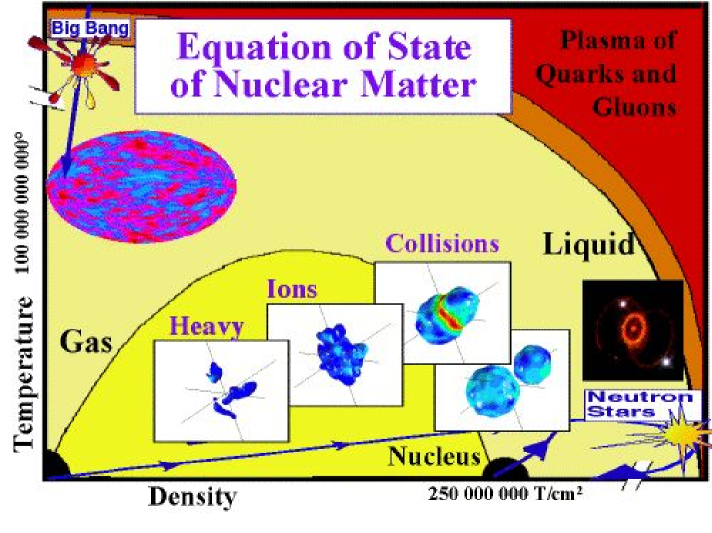
Figure 1: The phase diagram of dense matter. At high energy or density one can see the quark-gluon plasma while around the nuclear matter saturation point the liquid-gas coexistence region is shown. The trajectories followed by different cosmic events are sketched: the big-bang, the collapse of a supernova core in a neutron star and a heavy ion reaction.

At lower energy one expects a different type of phase transition namely the transition between particles and nuclei [1]. This condensation is analogous to a liquid-gas phase transition because of the resemblance between the nuclear force and a Van der Waals interaction with a long range attractive potential and a short range repulsive core. This phase transition plays an important role during the collapse of supernovae in neutron stars. On earth, physicists study it in nuclear reactions such as heavy ion collisions. Fantastic progresses have been achieved during a decade and especially in the past two years so it is the time to put together all the signals of the liquid-gas transition in order to see if they draw a consistent picture. As we will see each signal may have its own weak point and so is hardly a definitive proof taken individually. However, considered as a whole, the ensemble of observations becomes a rather strong piece of evidence for a phase transition.

2 Something is happening

As a matter of fact, in the macroscopic world the phase transitions manifest themselves by abrupt transformation of the system properties. Therefore one may be tempted to first look for rapid modifications of physical properties. In the past, many such fast transitions have been accumulated [2-6]. Some of them are summarized in figure 2. When the excitation energy of the system is increasing one observes the disappearance of the heavy residue in the decay products of the reaction. For heavy systems, this corresponds to an abrupt end of the binary fission. Those channels are in fact replaced by an abundant production of fragments, which in turn rapidly disappears in favor of the complete vaporization of the composite system. Simultaneously, one observes the onset of the radial expansion and the associated shortening of the breaking time. All these sudden changes in the behavior of the heavy systems recall the occurrence of a liquid-gas phase transition. However, they are not enough to demonstrate it and a deeper study is called for. Let us first review the theoretical tools needed to understand what is happening.

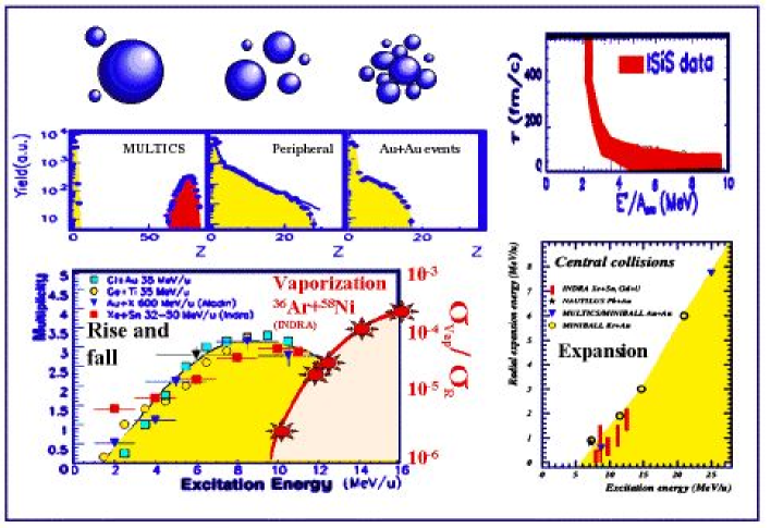
Figure 2: Compilation of many signals of ”something is happening” when a nuclear system is more and more excited. The left top part is the fragment distribution from ref. [11] showing the disappearance of the heavy fragment. Middle the multiplicity of fragments with Z¿2 (IMF) (left scale) demonstrating that the heavy residue is replaced by an abundant production of fragments (the multifragmentation) which are in turn replaced by the vaporization as shown by the cross-section for the total vaporization (right scale). Below, Dalitz plot (the charges of the three largest fragments are the three distances to the edges) from the Nautilus collaboration showing that the dominant channel for the decay of heavy hot nuclei which is normally the fission (left) is first replaced by the evaporation of IMF (middle) and then by the multifragmentation (right). This is confirmed by the ratio of the ternary and binary fission shown on the right (bottom). Above a compilation of the radial expansion demonstrating the onset of the nuclear explosion around 5-7 MeV excitation energy. Finally, the top right part shows a measure of the fragmentation time, which presents a clear decrease to become almost instantaneous above 3-5 MeV.

3 Dynamics of the reaction

3.1 Ab initio calculations

The first idea to control what is happening is to compare experimental results to dynamical simulation such as transport theory or molecular dynamics simulation. The nuclear reaction being very complex the easiest way to infer the phase diagram seems to directly study it from the model after fitting the various parameters on the multifragmentation data. This path towards the nuclear EOS is shown in figure 3. This would be the royal way if one would be sure to have the exact description of the reaction. However, up to now such a model does not exist and this path toward the observation of nuclear phases remains model dependent.

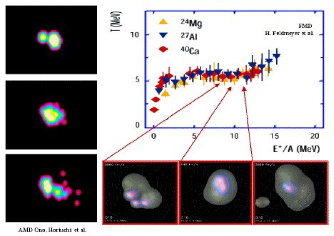
Figure 3: Molecular dynamics simulations of a collision (left ref. [7]) and of an equilibrium (right [8]). The deduced caloric curve for a confined hot Ca nucleus shows a plateau sign of a liquid-gas phase transition.

3.2 Dynamics of a phase transition

Being less confidant in the models, one may try to see direct signals of the considered dynamics and, if possible, of the phase transition in the data. In particular, many dynamical approaches are predicting that during the reaction the system may enter the unstable region of the phase diagram and thus can spontaneously undergo a rapid phase transition [1,9,10]. This spinodal decomposition is well known in many fields of physics. Indeed, deep inside a coexistence region uniform systems are generally unstable against fluctuations of the associated order parameter. This corresponds to mechanical instability for the liquid-gas phase transition or chemical instabilities for the mixing of two substances.

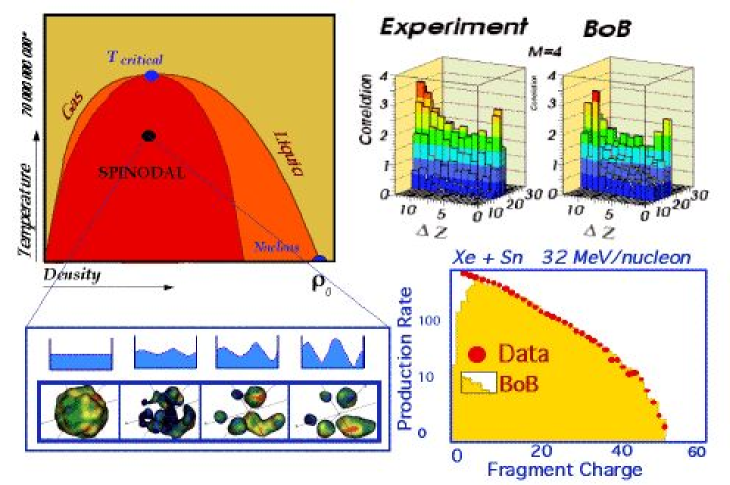
Figure 4: Schematic picture of the phase diagram (left top) showing the spinodal region in the coexistence zone. The small pictures below illustrate the amplification of density fluctuations schematically (above) and (below) as predicted by a stochastic mean-field approximation (Brownian one-Body approach (BoB)). The calculation is compared to the data on the right, for the fragment production measure by the INDRA collaboration for the Xe+Sn reaction at 32 MeV/nucleon (below) and for the associated correlation (above). The correlation corresponds to a sorting of events according to their average and fluctuation of the fragments (Z¿2) sizes. The peak at very small fluctuation may be an indication of a favored production of equal size fragments.

In particular, it can be shown that because of the finiteness of the nuclear forces and of the length imposed by the quantum Heisenberg uncertainty principle such instabilities presents a favored wave length [10]. This favors the breaking of the system in equal size fragments. In the past decade a lot of efforts have been devoted to the description of such spinodal decomposition in particular using stochastic mean-field approaches [10]. It was shown that because of the finiteness of the system and of the chaos induced by the non linear regime, which follows the early growth of instabilities, such characteristic is strongly washed by the end of the dynamics. However, one may try to spot some remains of this tendency to split in equal size fragments looking at correlations in the fragment distribution. The comparison of experimental data with the predictions of stochastic mean-field approaches has been recently performed [9]. It was shown that fragment distributions, as well kinematical observables and correlations are well reproduced by the model. Moreover, a ”fossil” signal of spinodal decomposition have been reported in the dispersion of the fragment sizes [9] (see figure 4).

3.3 Dynamics of statistics

However, it should be noticed that many approaches are able to do an almost equally good job as far as the majority of the multifragmentation observables are concerned. This is the case of many dynamical calculations involving very different approximations such as molecular dynamics approaches and stochastic mean-field. Even statistical approaches assuming the existence of a freeze-out stage in the reaction often fit well the data. This pleads in favor of a dominant importance of the phase space irrespectively of the considered dynamics. Indeed, the S matrix toward different macro-states always contains a micro-state degeneracy factor. Since this number varies by huge amount it might well be the dominant factor. Moreover, if the dynamics is sufficiently chaotic/mixing a uniform population of phase space might be achieved leading to a statistical distribution. Therefore one may try to study the reaction using statistical mechanics tools.

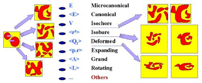
Figure 5: Schematic illustration of a dynamical evolution of a system into a statistical ensemble when many events are considered and when the dynamics is sufficiently chaotic. Now depending upon the pertinent observable imposed by the dynamics or the event sorting one should describe this set of data using different statistical ensembles some of them being illustrated on the right.

The use of static statistical physics approach to treat a dynamical process deserves some additional comments (see figure 5). Indeed, when studying nuclear reactions, it is clear that we are facing a dynamical process occurring during a finite time. Therefore one should not imagine that the statistical physics picture describes an equilibrium in the sense of an ergodic evolution of a unique event: the long term behavior (or time average) of a long-lived (infinite) system which eventually explore the whole phase space. The justification of the use of statistical physics to describe transient systems is the fact that an ensemble of event, taken at a time, which may fluctuate, from one event to another, corresponds to a statistical ensemble. Of course the dynamics remains essential in such approach since it determines the global variables characterizing the ensemble of events. The statistical physics idea is then that these global variables are the only important information, the more detailed description being governed by randomness.

It should be stressed that the pertinent information can be the result of the dynamics or of the observation process. Indeed, if the experimentalists are sorting the events according to a specific observable one should take into account this selection of event in the theoretical modeling. The application of information theory automatically leads to the description of the system as a statistical ensemble. Then it should be noticed that many different ensembles can be considered depending upon the pertinent information imposed by the dynamics and the event sorting. For example, if the dynamics allows the energy to fluctuate freely one may try to use the canonical ensemble. However, if the energy is conserved or if the events are sorted according to their energy one should use a microcanonical description. The same discussion can be made for the number of particles or the volume. Let us take the example of the volume. If the reaction occurs in a fixed volume (i.e. in a box) or if the events can be sorted according to their actual volume one should go for an isochore ensemble. Conversely if the volume fluctuates from event to events in such a way that at most only an average volume can be defined one should rather use an isobar picture. Finally one should stress that with such a picture of an ensemble of events one can also build the statistical description of an evolving system such as the rotating or the expanding systems. This only corresponds to the introduction of a time odd observable as a constraint in the maximization of the entropy.

4 Signals of a phase transition

In the past years many new analyses have been performed often based on novel ideas in order to put in evidence the liquid-gas phase transition in nuclei. Let us briefly review the most recent and original ones.

4.1 Critical behaviors, the gas side

Phase transitions are known to be related to critical behaviors and to be ruled by universal properties. In particular, at the critical point the system presents a fractal structure and so scaling should hold. This leads for example to the famous power law shape of the fragment size distribution. Moreover, using renormalization group argument one can relate the fragment yield and the distance to the critical point. Indeed, a yield for a given size at a given distance to the critical point is proportional to the yield of a different size at a scaled distance. These critical behaviors have been identified in many nuclear reactions (see figure 6) [11,12]. The inferred critical exponents are in reasonable agreement with those expected for the liquid-gas phase transition.

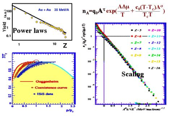
Figure 6: The top-left figure a typical fragment size distribution fitted by a power law indicating the proximity of a critical point. Right the special form of the fisher scaling [14] as tested experimentally in ref. [15]. The resulting scaling function is shown below the equation. The deduced phase diagram is shown on the left (see text).

Recently, it has been proposed [15] to test the specific scaling proposed by Fisher [14]. This scaling is based on the simple idea that a real gas of interacting particles can be considered as an ideal gas of clusters in chemical equilibrium. This can be seen as the basis of many multi-fragmentation models except the fact that they often take the excluded volume into account. Then the population of the various species can be evaluated according to their associated free energy. This normally contains a volume and a surface term. When the gas is in contact with the liquid the volume term is proportional to the difference of chemical potential between the liquid and the gas. When the liquid is in equilibrium with the gas this term drops off. The surface term is proportional to the surface tension which is supposed to decrease and eventually to go to zero as we get closer and closer to the critical point. Finally, a logarithmic factor is included in the free energy functional in order to account for the fractal structure of the fragments at the critical point. This topological contribution leads to the famous power law distribution of fragment size at the critical point.

The Fisher scaling gives a specific recipe in order to scale all the observed fragment yields on a single curve. This scaling have been recently tested with an amazing success on pion-induced fragmentation data [15] (see figure 6). Taking the analogy of the perfect gas of cluster seriously, the authors of ref. [15] proposed to compute all the thermodynamical quantities using the perfect gas equations of state. For example, the partial pressure $P_{A}$ induced by the fragments A is proportional to $n_{A}T$. The various pre-factors and in particular the volume is eliminated by taking the ratio with the thermodynamical quantities evaluated at the critical point. This imposes that the volume of the considered system is identical to the one of the critical point. In such a way, putting the difference of chemical potential between liquid and gas to zero one gets the coexistence line as shown on figure 6 (see ref [15] for more details).

The full understanding of this signal of a phase transition needs more theoretical and experimental work. First of all, we have recently shown that, in very small system, a critical behavior should be expected along a line inside the coexistence region [14]. This property can also be rather sensitive to the coulomb field. Finally the idea that the thermodynamics of a complex real gas can be treated as a superposition of clusters ideal gas should be checked (see also the chapter about the caloric curve). In this respect the role of the total volume of the system and of the volume excluded by each fragment should be clarified. However, the observed scaling is certainly an interesting signal of a critical behavior.

4.2 Critical behaviors, the liquid side [16]

In finite systems not only the small fragment (gas) distribution can be studied but also the largest fragment (liquid) can be measured. It has been recently discussed that the scaling behavior of this distribution may also signal phase transitions [16] of the aggregation type. Indeed, within the aggregation scenarios, to which belongs the liquid gas phase transition, the order parameter is expected to be the size of the largest fragment. Then in ref. [16] it is shown that the scaling characteristic of the distribution of order parameter should change when passing from one phase to the other. More precisely, the order parameter distribution should follow a $\Delta$ -scaling with $\Delta$ =1/2 in the coexistence (second scaling) and $\Delta$ =1 above the critical point (first scaling). These scaling can be seen as very general scaling of the probability distribution of the largest fragment size using only two parameters e.g. its maximum (or average) and its width. Then, if the maximum is taken as a reference and if the standard deviation is used as a unit, the probability, correctly normalized to take care of the unit change, might become a scale invariant function. For example, with such a procedure all the Gaussian distributions collapse onto a single universal curve. Such a scaling indicates some relation between the processes associated with various distributions, which follow the same scaling. For example, all the processes, which fulfill the Laplace central limit applicability conditions, pertain to the Gaussian universality class.

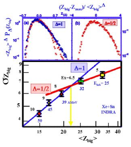
Figure 7: Bottom, the fluctuation of the size of the largest fragment as a function of its average value (both in log scale) as measured by the INDRA collaboration for the central events of the Xe + Sn at 5 incident energies (written bellow the points) corresponding to 5 different excitation energies per nucleons of the composite system (written above the points). The two lines show the proposed linear and square root behavior and the arrow shows the assumed point of the phase change. Above are shown two tests of the scaling of the whole distribution using the maximum as the center and the square root of the average as a scale (right) or the average as a scale (left). On the right only the two first energies are shown confirming the second scaling while on the left these energies are shown in a light grey while the three higher energies are in black. Again the black points scale well but not the others demonstrating that only the three highest energies presents a first scaling.

As far as the search for phase transition is concerned, the key point is then how the fluctuation changes with the system size or equivalently with the maximum or the average of the distribution. If the standard deviation scales as a power law of the average then the power is called $\Delta$ . A second scaling ($\Delta$ =1/2) is then the rather usual type of fluctuations which goes like in the random walk as the square root of the average. The first scaling $\Delta$ =1 corresponds to a faster increase of the fluctuations linearly with the mass. The fact that it dominates out side the coexistence region can be understood since in that case the largest fragment is only the largest one among several fragments of comparable small size, i.e. it belongs to the gas phase. Therefore, its fluctuations are determined by the fact that it should be larger than the second largest fragment. Conversely, in the coexistence region the largest fragment is the liquid body, which will become infinite at the thermodynamical limit. Its fluctuations are ruled by the equilibrium with the gas and so look like the one of a random walk process.

Figure 7 presents the fluctuation of the largest fragment size as a function of its averaged value for the central events of the Xe + Sn reaction at 5 incident energies [16]. Two behaviors seem to be observed: while for the low energy the largest fluctuation seems to behave like the root of the average (second scaling), the high energy points rather exhibit a linear dependence (first scaling). This observation is confirmed by the analysis of scaling of the distribution of sizes (figure 7). This would plead in favor of a phase change just above 32 MeV/nucleon incident energy i.e. about 7MeV excitation energy.

A lot of work is needed before reaching a definite conclusion from this signal alone. Indeed, one should study in detail the transition region to try to identify how the system goes from one phase to the other. Moreover, since the tails of the distribution are important for the scaling one should improve the statistics. Also the number of energy points should be enlarged as well as other systems analyzed. The characterization of ”single source” (central) events as a function of the bombarding energy should be studied. The role of conservation (mass, energy…) should be investigated using for example different models. Finally, since this signal is expected for many cases from geometrical fragmentation (percolation) to dynamical scenarios such as gelation passing by thermodynamical systems such as phase transitions (Ising model) one should find other observables in order to get a deeper insight into the observed phenomenon.

4.3 Flattening of the caloric curve

In order to get a direct information about the nuclear phase diagram and the associated equation of states one should look for direct thermodynamical information. In the past year there have been many attempts to test if a thermal equilibrium was a reasonable approximate description of the fragmenting systems [17-20]. The first indication of such an adequacy of a statistical description of a freeze-out configuration is given by the amazing success of statistical models. However one may look for a direct experimental evidence of such an equilibrium at a given stage of the reaction.

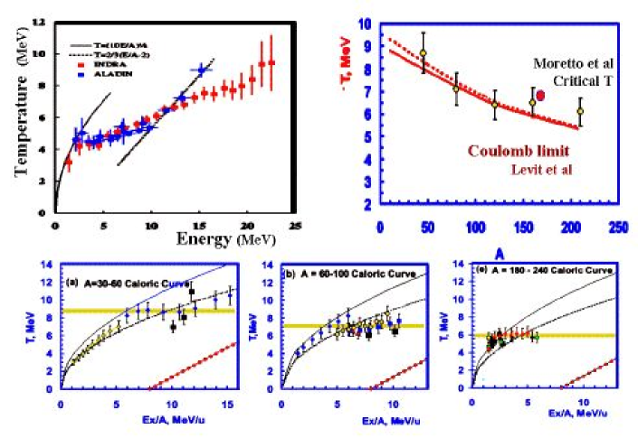
Figure 8: Top-left the caloric curve of the Aladin group [17] compared with the one measured by the indra collaboration [18]. Bottom, caloric curves for different mass of the fragmenting systems coming from many different experiments as analyzed in ref. [20]. The observed mass dependence of the onset of the flattening of the caloric curves is reported in the top-right figure. The point is the critical point discussed in the subsection 1 coming from ref. [15]. The lines are the limiting temperatures due to the Coulomb instabilities derived in ref. [21].

The first result of the Aladin group presenting evidences for a phase transition as an almost constant temperature over a broad range of energies have triggered a lot of activities (see figure 8). Different thermometers were tested, the slope (or the average) of the kinetic energies (kinetic temperature), the population of various isotopes (chemical temperature) and the ratio between excited states population (internal temperature). At the beginning the different thermometers and different experiments seemed to not be in agreement. However, now, the various observations start to draw a coherent picture and the different thermometers agree within the experimental error bars as soon we take into account important physical effects as:

• i) the fact that clusters are not an ideal gas but have a cluster- and even state-dependent excluded volume [18];

• ii) the fact that the radial expansion affects the kinetic temperature both because of the global boost but also because of the possible fluctuation of the radial velocity;

• iii) the fact that after the freeze-out the fragments should cool down leading to a modification of the various population of clusters and excited states (side feeding) [19],

• iv) the fact that in a hot environment the various states get life times which broader their excitation energy affecting their relative populations.

Recently, it has been shown that the mass of the fragmenting system has also an influence on the observed caloric curve [20]. When unfolding the effect of the mass the authors of ref. [20] show that the caloric curves are less dispersed and present a plateau behavior. The temperature of the observed plateau decreases with the mass of the fragmenting system. It is interesting to note that the critical temperature discussed in the subsection 1 above just lies on the curve of the plateau temperature as a function of the mass. The authors of ref. [20] have compared the observed mass dependence of the temperature plateau with the maximum temperature for the existence of a charged nucleus in equilibrium with a gas computed in ref. [21]. It should be noticed that above this onset of Coulomb instabilities only a fragmented system may exist. The amazing agreement shown in figure 8 pleads in favor of a relation of the observed modification of the trend of the caloric curve with the onset of Coulomb instabilities.

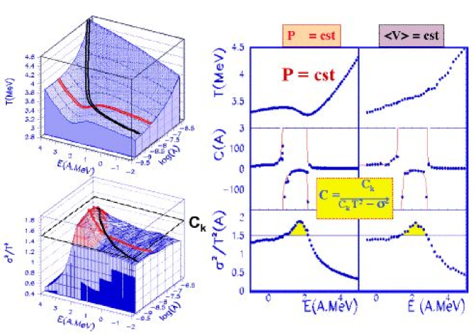
Figure 9: Results from a microcanonical Lattice-gas model with a constraint only on the average volume [22]. Top left the temperature as a function of the energy and the Lagrange multiplier ($\lambda$) which can be seen as a pressure times a temperature. On this curve on the temperature surface are shown two transformations one at constant pressure the other one at constant volume. The corresponding caloric curves are shown on the right. Bottom left the kinetic energy fluctuations for each statistical ensembles characterized by an energy and a Lagrange multiplier. The dotted line marked Ck is the canonical expectation. The curves are the isobar and isochore transformations leading to the two curves shown on the right. Above is the heat capacity of the considered ensemble either computed from the thermodynamics (line) or reconstructed using the kinetic energy fluctuations as expressed in the inserted equation.

Of course here too a lot of work remains to be done to strengthen the argument. Of particular interest is the behavior of the curve at high excitation energy as well as a precise study of the observed flattening. It should be stressed that from the theoretical point of view in the case of a liquid-gas phase transition one do not expect that the phase transition should be marked by a specific behavior of the caloric curve. Indeed, the order parameter of the liquid-gas phase transition is the density i.e. the volume. Then, the caloric curve is not a single curve but a bi-dimensional equation of state depending both on energy and volume (or pressure); therefore the caloric curve depends upon the actual condition defining the volume as illustrated in figure 9 for the lattice-gas model with a volume constrained only in average from ref. [22]. However, it should be noticed that, while in models the volume can be freely changed, in actual nuclear reactions it is determined by the dynamics and cannot be controlled but might possibly be measured.

4.4 Abnormal kinetic energy fluctuations and negative heat capacity

In ref. [22] it has been proposed to use the kinetic energy fluctuation of events sorted in total energy to directly infer thermodynamical quantities and more precisely the ensemble heat capacity. Indeed, from a classical point of view, for an ensemble at constant energy (microcanonical ensemble), the sharing of energy between the kinetic and the interaction part should be governed by the respective entropies. Then the most probable partition should correspond to an equal temperature while the fluctuation should depend upon the respective heat capacities. Knowing the kinetic heat capacity one can then infer the interaction one and so the total one as well as the sum of both (see the equation in figure 9 and ref. [22] for more details).

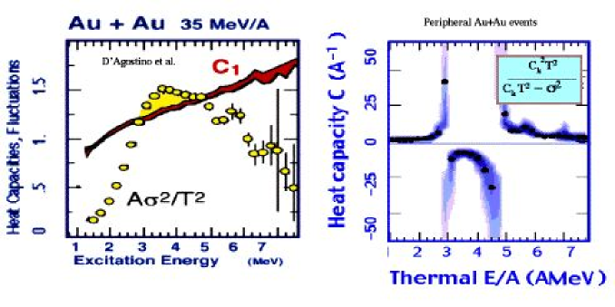
Figure 10: From[27] on the left the kinetic fluctuations divided by the temperature square (dots) compared with the kinetic heat capacity (thick line) on the right the deduced total heat capacity.

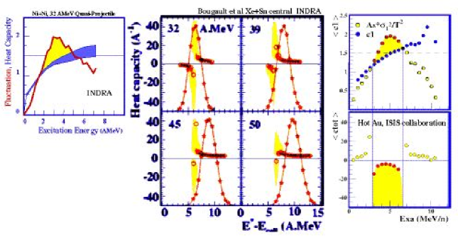
Figure 11: Left the kinetic energy fluctuation divided by the square of the temperature from peripheral Ni+Ni reaction at 32 MeV/A (INDRA collaboration [28]) the thick line is the kinetic energy heat capacity. Middle, reconstructed heat capacity from the central events of the Xe+Sn reaction at four different incident energies[28]. Right, top the fluctuation (as in the left curve) and below the deduced heat capacity from the pion reaction on Gold discussed in the subsection 1 [29].

Moreover, it is shown in ref. [22] that in a microcanonical system for which the volume is not defined through boundary conditions as it is the case for the fragmentation of open systems the phase transition is associated with the occurrence of a negative heat capacity.

Negative heat capacities seem impossible from the thermodynamical point of view. However, they have been discussed first in the astrophysical context [23] of self-gravitating systems. Recently they have been pointed out as a possible generic behavior of mesoscopic systems undergoing a phase transition, such as in metallic clusters [24] and in nuclei [25]. It was recently shown that this concept should be extended to inverted curvature of thermodynamical potentials as a function of any variables related to the order parameter [22]. It should be noticed that the occurrence of negative heat capacities has recently be reported for clusters [26]. With the nuclear physics results, this is the first experimental evidence for such an anomalous behavior.

Coming back to the kinetic energy fluctuations as a measure of the heat capacity it is shown in ref. [22] that a negative heat capacity can be spotted as a microcanonical kinetic energy fluctuation becoming larger than the expected canonical limit. Indeed, in the equation which relates the heat capacity to the kinetic energy fluctuation (see figures 10 and 11) one can see that the denominator is the difference between the canonical expectation $C_{k}T^{2}$ and the observed fluctuation. When the latter becomes larger than the former the heat capacity diverges before becoming negative.

This signal of a phase transition has been looked for in experiments. In such a case an easy splitting of the energy is between the thermal excitation and agitation on one side and the partition Q-value plus the Coulomb interaction on the other side. The expected canonical prediction can be inferred from the relation between the average kinetic energy and the temperature since this provides $C_{k}$. Figure 10 shows the first experimental results of a fluctuation overcoming the canonical expectation with the corresponding deduced heat capacity for an excited gold nucleus [27].

Figure 11 presents an ensemble of results coming from different reactions at different energies measured with the Indra [28] and Isis [29] apparatuses all presenting abnormally large kinetic energy fluctuations and consequently negative heat capacities.

Also for this novel signal of phase transition a lot of work is needed both from the experimental and theoretical point of view. First many things must be known in order to perform a good total energy sorting and to reconstruct the kinetic energy fluctuations at freeze out. These reconstructions often need hypotheses such as the volume of the freeze-out and the origin of emitted particles. Additional measurements to control these hypotheses have to be performed. However, kinetic energy fluctuations are a promising way to infer thermodynamical properties and to signal phase transitions.

4.5 Fractionating distillation of neutron rich matter

In ref. [30] it has been discussed that, since the nuclear matter is composed of two fluids, neutrons and protons, the liquid-gas phase transition should lead to a distillation phenomenon. Indeed, looking at the phase diagram as a function of the chemical proportion of neutrons and protons y=N/A one can see (figure 12) that, except for symmetric nuclear matter, the isospin content of the gas and of the liquid is different. The liquid tries to come back to the symmetric matter while the gas absorbs the remaining enriched matter. In ref. [32], using the lattice-gas model, it was shown that this distillation should strongly influence the light fragment production. For example, figure 12 shows that for a neutron rich system undergoing a phase transition the enrichment in neutron rich isotopes (such as the tritium) compared to neutron poor ones (e.g. Helium-3) can be much larger than expected on the basis of the N/Z of the source.

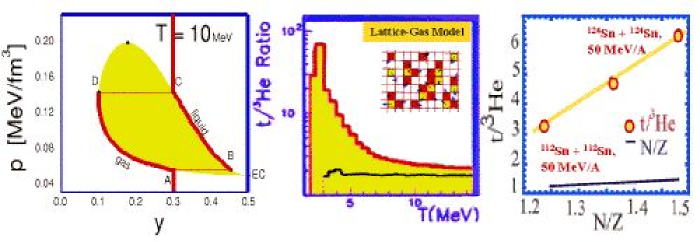
Figure 12: Left the coexistence region at constant temperature in the pressure/neutron-proportion plane [30]; the thick line is an isothermal transformation. As the pressure reduces the system may reach the coexistence region in C then the liquid goes from C to B, while the gas appears very neutron rich in D and then goes to A. In A the liquid gas transformation is done. Middle, the tritium to helium-3 ratio as a function of the temperature [31]. In the coexistence region below T=6MeV one observes a very strong relative population of neutron rich isotopes. The black line is the result in absence of an isospin dependent interaction term. In such a case the ratio is nothing but the N/Z. Right, the experimental ratio observed for the central events of different reactions involving two isotopes of Sn at 50 MeV/A bombarding energy [32]. The same strong enrichment is observed.

This strong enrichment together with a clear indication of chemical equilibrium have been recently reported [33] and interpreted as a signature of the fractionation phenomenon. This is a promising avenue for the determination of the nuclear equation of state and phase diagram. Of particular importance is the isospin dependence of the nuclear equation of state, the determination of which can benefit from this distillation signal (see also ref. [33] for more details).

5 Conclusions and discussion

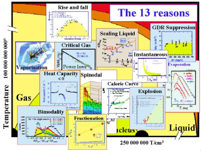
Figure 13: Sketch of the 13 signals of the nuclear liquid gas phase transition (see text).

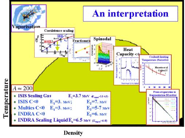
Figure 14: Summary of the recent signals discussed in this review article placed on a possible trajectory of the nuclear systems in the density temperature plane. First at low energy we are in presence of a saturating vapor around the nucleus and one observe the Fisher scaling. Then at a critical temperature the system cannot sustain the Coulomb repulsion and dives into the coexistence zone imposing a mass-dependent bending of the caloric curve. Reaching the spinodal the heat capacity becomes negative and some signal of the spinodal decomposition at the origin of the fragment production may remain. In this region one observe also a fractionation of the neutron rich matter. Then exciting the coexistence it encounters the second divergence of the heat capacity and the end of the second scaling of the largest fragment. Then it will gradually go towards a complete vaporization. The table gives, for a mass around 200, the excitation energies at which each signal occurs. One can see that they consistently point toward two energies, which might be the entrance and the exit of the coexistence region.

In this review, we have shown that many signals of the liquid-gas phase transition have been observed up to now. In figure 13, we have collected 13 such evidences:

• i) the evaporation of light particles which can be seen as the emission of a gas from an isolated piece of matter with no external saturating pressure [2-4]

• ii) the suppression of the giant dipole vibration marking the end of a collective behavior [6] marking the boiling point which for a Sn nucleus occurs around 5 MeV temperature (2.5 MeV excitation energy per nucleon).

• iii) the onset in the same temperature domain of an instantaneous fragmentation [2-5]

• iv) the bending of the caloric curve again in the same temperature domain [17-20]

• v) as well as the observation of critical behavior for the gas fragments [11-15]

• vi) and the onset of the nuclear explosion with a fast radial expansion [2-5]

• vii) then one observe some fossil signal of a spinodal breaking in equal size fragments [9-10]

• viii) and at the same time the kinetic energy fluctuation becomes abnormal a phenomenon which can be related to the presence of a negative heat capacity [22-29]

• ix) together with a fractionation which looks like equilibrated [30-33]

• x) in this energy domain many bi-modalities of the event distribution as a function of various observables are observed as suggested in [35] as a signal of phase transition, such as in the difference between the mass contained in the fragments and in the light particle [34] or in the plane corresponding to the two largest fragment masses [2].

• xi) then after the rise of the production of large fragments it is the time of its fall [2-4]

• xii) the scaling of the large fragment mass distribution then passes from the second to the first type [16]

• xiii) Finnally one observes an equilibrated vaporization [2,3,18]

Taken individually each of these 13 signals has its own drawback and weakness. However, taken as a whole they start to draw a convicting picture of the actual observation of the liquid-gas phase transition in nuclei. Not only the reported signals are qualitative they are becoming event quantitative (as illustrated on figure 14) allowing to think about a real metrology of the nuclear phase diagram. This is a good news because a lot remains to be done since not only the coexistence zone of the symmetric matter should be measured but also the isospin dependence which starts to be experimentally accessible thanks to the new radioactive beam factories.

6 REFERENCES

1.  Siemens P.J., Nature 305 410 (1983), Bertsch G.F. and Siemens P.J., Phys. Lett. B126 9(1983)

2.  Lopez O., Nucl. Phys. A685 246( 2001) and refs. there in.

3.  Durand D., Tamain B. and Suraud E., ”Nuclear Fragmentation” IOP-Publishing 2000 and refs. there in.

4.  Das Gupta S. et al, nucl-th/0009033 and refs. there in.

5.  Beaulieu L. et al, nucl-ex/0004005, Lefort T. et al, nucl-ex/9910017

6.  Piattelli P. et al, Nucl. Phys. A599 63c(1996)

7.  Ono A. et al., Phys. Rev. C48 2946(1993)

8.  Schnack J. and Feldmeier H., Phys. Lett. B409 6(1997) and Feldmeier H. private comunication

9.  Borderie B. et al, nucl-ex/0102015 and Phys. Rev. Lett. 86 3252(2001)

10. Guarnera A. et al, Phys. Lett. B403 191(1997) , Chomaz Ph. et al, Phys. Rev. Lett. 73 3512(1994)

11. D’Agostino M. et al, Nucl. Phys. A650 329(1999); and Elliott J. B. et al, Phys. Rev. Lett. 85 1194(2000)

12. Campi X., Phys. Lett. B208 351(1988)

13. Fisher M.E., Physics 3 255(1967)

14. Gulminelli F. and Chomaz Ph., Phys. Rev. Lett. 82 1402(1999)

15. Moretto L. et al, present proceedings and Elliott J. B. et al, nucl-ex/0104013

16. Botet R. et al, nucl-ex/0101012 and Phys. Rev. E62 1825(200)

17. Pochodzalla J. et al, Phys. Rev. Lett. 75 1040(1995)

18. Gulminelli F. and Durand D., Nucl. Phys. A615 117(1997) and ref. there in.

19. Tsang B. et al, Phys. Rev. C53 R1057(1996)

20. Natowitz J. et al, nucl-ex/0106016

21. Bonche P. et al, Nucl. Phys. A427 278(1984) and A436 265(1986)

22. Chomaz Ph. and Gulminelli F, Nucl. Phys. A647 153(1999), to be published in Phys. Rev. Lett. (2001)

23. Lynden-Bell M., Physica A263 293(1999); Hauptmannet H. al, Am. J. Phys. 68 421(2000)

24. Labastie P. et al, Phys. Rev. Let. 65 1567(1990)

25. Gross D. H. E., Phys. Rep. 279 119(1997)

26. Schmidt M. et al, Phys. Rev. Lett. 86 1191(2001)

27. D’Agostino M. et al, Phys. Let. B473 219(2000), nucl-ex/0104024 to appear in Nucl. Phys. A (2001) and D’Agostino M. private communication

28. Bougault R. et al, private communication.

29. Lefort T. et al, private communication.

30. Muller H. and Serot B. D., Phys. Rev. C52 2072(1995)

31. Chomaz Ph. and Gulminelli F., Phys. Lett. B447 221(1999), Pan J. and Das Gupta S., Phys. Rev. C57 1839(1998)

32. Verde G. et al, Nucl. Phys. A681 299c and 323c(2001), Xu H. S. et al, Phys. Rev. Lett. 85 716(2000)

33. Chomaz Ph., Nucl. Phys. A681 199c(2001)

34. Borderie B. et al, nucl-ex/0106007

35. Chomaz Ph., Gulminelli F. and Duflot V., Phys. Rev. E (2001) to be published