Probing jet properties via two particle correlation method

Abstract

The formulae for calculating jet fragmentation momentum, $\left<j_{T}^{2}\right>$, and parton transverse momentum, $\left<k_{T}^{2}\right>$, and conditional yield are discussed in two particle correlation framework. Additional corrections are derived to account for the limited detector acceptance and inefficiency, for cases when the event mixing technique is used. The validity of our approach is confirmed with Monte-carlo simulation.

1 Introduction

In pp, pA or AA collisions at RHIC, the high $p_{T}$ part of the hadron spectra is dominated by the two-body hard-scattering process. In this process, the two scattered partons typically appear as a pair of almost back-to-back jets. The properties of the di-jet system can be characterized by the jet fragmentation momentum, $j_{T}$, the parton transverse momentum, $k_{T}$, and the fragmentation function, $D(z)$. Specifically, $j_{T}$, $k_{T}$ and $D(z)$ describe the spread of hadrons around the jet axis, the relative orentation of the back-to-back jets and the jet multiplicity, respectively.

Traditionally, energetic jets were reconstructed directly using standard jet finding algorithms[1, 2]. In heavy-ion collisions, due to the large amount of soft background, direct jet reconstruction is difficult. Even in pA or pp collisions, the range of energy accessible to direct jet reconstruction is probably limited to $p_{T}>10$ GeV [3], below which the ‘underlying event’ background contamination become important. The situation is even more complicated for finite acceptance detectors like PHENIX due to the leakage of the jet cone outside the acceptance.

The two-particle-correlation technique provides an alternative way to access the properties of the jet. It is based on the fact that the fragments are tightly correlated in azimuth $\phi$ and pseudo-rapidity $\eta$ and the jet signal manifests itself as a narrow peak in $\Delta\phi$ and $\Delta\eta$ space. The jet properties are extracted statistically by accumulating many events. This method was initially used in 70’s in searching for jet signals in pp collisions at CERN ISR [4, 5, 6]. It overcomes problems with the underlying event background, probes the jet signal at lower $p_{T}$, and has recently excited renewed interest at RHIC [7, 8, 9].

Experimentally, jet measurement is challenging due to detector inefficiency and limited experimental acceptance. A certain fraction of jet pairs is lost either because the track is not found or because part of the jet cone falls outside the acceptance. The average jet pair detection efficiency can be estimated statistically using event mixing technique. The main goal of the paper is to establish the procedures for measuring the jet shape and jet multiplicity independent of the detector efficiency and acceptance.

The discussion is split into three sections. In Section.2, we lay out the formulae for extracting $j_{T}$, $k_{T}$ and conditional yield. In the interest of space, the reader is encouraged to see Ref.[9, 10] for more details on the definition of the variables. In Section.3, we discuss the event mixing technique necessary in correcting for limited acceptance and inefficiency, where we use the PHENIX detector as an example. We discuss separately the two dimensional ($\Delta\eta$, $\Delta\phi$) and one dimensional ($\Delta\phi$) correlation and derive the normalization factors for the conditional yield in each case. In Section.4 we verify the procedure of correcting for finite acceptance with Pythia simulation.

2 Some formulae

2.1 Formulae for $j_{T}$, $k_{T}$

Fig.1 illustrates the single jet fragmentation (left panel) and away side jet fragmentation (right panel). The jet fragmentation momentum, $j_{T}$, and parton initial momentum, $k_{T}$, determine the relative orientation of the fragmented hadrons. $j_{T}$ and $k_{T}$ are vectors, their projection in the azimuthal plane perpendicular to the jet direction are denoted as $j_{T_{y}}$ and $k_{T_{y}}$. For single jet fragmentation, if we denote $\Delta\phi$, $\phi_{tj}$, and $\phi_{aj}$ as the angles between trigger-associated, trigger-jet and associated-jet, respectively, then the following relations are true:

$$\Delta\phi=\phi_{tj}+\phi_{aj}\quad \quad\sin(\Delta\phi)=\frac{p_{out,N}}{p_{T,asso}}\quad,$$ ,

$$\sin(\phi_{tj})=\frac{j_{T_{y},trig}}{p_{T,trig}}\equiv x_{j,trig}\quad \quad\sin(\phi_{aj})=\frac{j_{T_{y},asso}}{p_{T,asso}}\equiv x_{j,asso}\quad.$$ , (1)

Here $p_{out,N}$ is the component of associated particle $p_{T}$ ($p_{T,asso}$) perpendicular to the trigger particle $p_{T}$ ($p_{T,trig}$). Assuming $\phi_{tj}$ and $\phi_{aj}$ are statistically independent, we have (cross terms average to 0),

$$\left<{\sin^{2}\Delta\phi}\right>=\left<{\sin^{2}\phi_{tj}\cos^{2}\phi_{aj}}\right>+\left<{\sin^{2}\phi_{aj}\cos^{2}\phi_{tj}}\right>$$ (2)

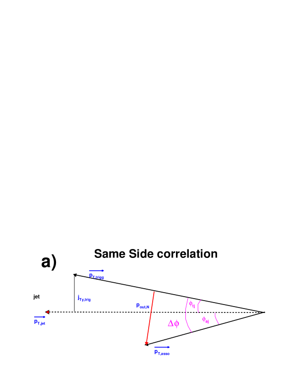
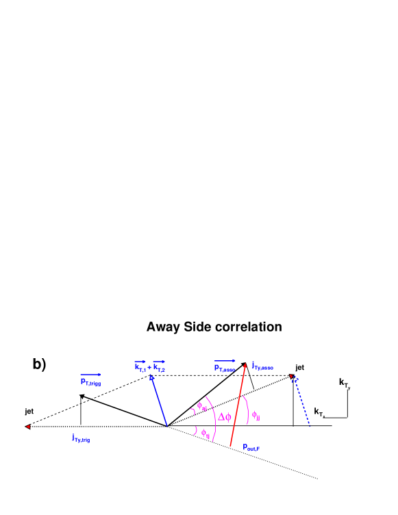
Figure 1: Schematic view of jet fragmentation. a) same side jet, b) away side jet.

Similarly for the far-side correlation, we have

$$\Delta\phi = \phi_{tj}+\phi_{aj}+\phi_{jj}\quad,\quad\sin(\Delta\phi)=\frac{p_{out,F}}{p_{T,asso}}\quad,$$ (3)

where $\phi_{jj}$ represents the angle between the two jets. Expanding $\sin^{2}\Delta\phi$ and dropping all cross terms (which average to 0), we get

$$\left<{\sin^{2}\Delta\phi}\right> = \left<{\left(\sin\phi_{tj}\cos\phi_{aj}cos\phi_{jj}\right)^{2}}\right>+\left<{\left(\sin\phi_{aj}\cos\phi_{tj}cos\phi_{jj}\right)^{2}}\right>+$$ (4)

$$\left<{\left(\sin\phi_{jj}\cos\phi_{aj}cos\phi_{tj}\right)^{2}}\right>+\left<{\left(\sin\phi_{tj}\sin\phi_{aj}sin\phi_{jj}\right)^{2}}\right>$$

Let’s define $z_{trig}=p_{T,trig}/p_{T,jet}$ and $x_{k}=\sqrt{2}k_{T_{y}}/p_{T,jet}=\sqrt{2}k_{T_{y}}z_{trig}/p_{T,trig}$. If $\phi_{jj}$ is small, or $p_{T,jet}\gg k_{T_{y}}$, then $\sin(\phi_{jj})\approx\left(k_{T_{y},trig}+k_{T_{y},asso}\right)/p_{T,jet}$, $i.e.$ $k_{T}$ only affects the jet direction. Thus statistically we obtain

$$\left<{sin^{2}(\phi_{jj})}\right>\approx 2\left<{\frac{k^{2}_{T_{y}}}{p^{2}_{T,jet}}}\right>=\left<{x_{k}^{2}}\right>\quad.$$ (5)

Substituting the $\sin$ and $\cos$ terms from Eq. 2.1 and 3 into Eq. 2 and Eq. 4, we obtain the equations for the RMS value of $j_{T_{y}}$ and $k_{T_{y}}$ (for a given variable $x$, $(x)_{RMS}\equiv\sqrt{\left<{x^{2}}\right>}$),

$$\left({j_{T_{y}}}\right)_{RMS}=\sqrt{{\left\langle{p_{out,N}^{2}}\right\rangle}\mathord{\left/{\vphantom{{\left\langle{p_{out,N}^{2}}\right\rangle}{1+\left\langle{x_{h}^{2}}\right\rangle-2\left\langle{x_{j,trig}^{2}}\right\rangle}}}\right.\kern-1.2pt}{\left(1+\left\langle{x_{h}^{2}}\right\rangle-2\left\langle{x_{j,trig}^{2}}\right\rangle\right)}}$$ (6)

$$\left(k_{T_{y}}z_{trig}\right)_{RMS}=\sqrt{\frac{{\left\langle{p_{out,F}^{2}}\right\rangle-\left\langle{p_{out,N}^{2}}\right\rangle\left({1-\left\langle{x_{k}^{2}}\right\rangle}\right)}}{2\left(\left\langle{x_{h}^{2}}\right\rangle-\left\langle{x_{h}^{2}x_{j,trig}^{2}}\right\rangle-\left\langle{x_{j,trig}^{2}}\right\rangle+2\left\langle{x_{j,trig}^{4}}\right\rangle\right)}}$$ (7)

where $x_{h}=p_{T,asso}/p_{T,trig}$. Assuming the $\Delta\phi$ follows gaussian statistics, a simple Taylor expansion connects $p_{out}$ with the jet width, $\sigma$:

$$\left<{p_{out}^{2}}\right> = \left<{p_{T,asso}^{2}sin^{2}\Delta\phi}\right>$$ (8)

$$\approx \left<{p_{T,asso}^{2}}\right>[sin\left<{\Delta\phi^{2}}\right>-\frac{\left<{\Delta\phi^{4}}\right>}{3}]$$

$$= \left<{p_{T,asso}^{2}}\right>[sin\sigma^{2}-\sigma^{4}]$$

By replacing the $p_{out}$ terms in Eq.2 and Eq.4, we can derive the relation between jet width and RMS value of $j_{T_{y}}$ and $k_{T_{y}}$.

Since Eq. 6 and Eq. 7 contain variables $x_{j,trig}$ and $x_{k}$ that depend on $j_{T_{y}}$ and $k_{T_{y}}$, we have to calculate $(j_{T_{y}})_{RMS}$ and $(k_{T_{y}})_{RMS}$ iteratively. However when trigger and associated particle $p_{T}$ are much larger than typical $j_{T}$ value, the near side jet width $\sigma_{N}$ is small and $x_{j,trig}\approx 0$. Hence Eq. 6 can be simplified to,

$$\left(j_{T_{y}}\right)_{RMS} \simeq \sqrt{\frac{sin\sigma^{2}_{N}\left<{p^{2}_{T,asso}}\right>}{1+\left<{x_{h}^{2}}\right>}}$$ (9)

For the far-side correlation, if the trigger $p_{T}$ is much larger than $k_{T_{y}}$ and $j_{T_{y}}$, then $\left<{x_{k}^{2}}\right>\approx 0$, $\left<{x_{j}^{2}}\right>\approx 0$ and Eq. 7 reduces to

$$\left({k_{Ty}z_{trig}}\right)_{RMS} \simeq \sqrt{\frac{\left<{p_{out,F}^{2}}\right>-\left<{p_{out,N}^{2}}\right>}{2\left<{x_{h}^{2}}\right>}}$$

$$\simeq \frac{1}{\sqrt{2\left<{x_{h}^{2}}\right>}}\sqrt{\langle p_{T,assoc}\rangle^{2}\sin^{2}\sigma_{F}-(1+\left<{x_{h}^{2}}\right>)\left(j_{T_{y}}\right)^{2}_{RMS}}$$

Previously, Ref [9] has derived the approximate relations between the $j_{T}$, $k_{T}$ and the measured jet width in the near side ($\sigma_{N}$) and the away side ($\sigma_{A}$) ($\left<{|a|}\right>$ is the mean of the $|a|$, $\left<{|a|}\right>^{2}=2/\pi\left<{a^{2}}\right>$):

$$\left<{|j_{T_{y}}|}\right> = \sqrt{2/\pi}{{\left\langle{p_{T,asso}}\right\rangle\sigma_{N}}\mathord{\left/{\vphantom{{\left\langle{p_{T}}\right\rangle\sigma_{N}}{\sqrt{1+\left\langle{x_{h}}\right\rangle^{2}}}}}\right.\kern-1.2pt}{\sqrt{1+\left\langle{x_{h}}\right\rangle^{2}}}}$$ (11)

$$\left<{|k_{T_{y}}z_{trig}|}\right> = \frac{1}{\sqrt{2}\left\langle{x_{h}}\right\rangle}\sqrt{\left<{p_{T,asso}}\right>^{2}\sin^{2}\sqrt{\frac{2}{\pi}}\sigma_{A}-(1+\left\langle{x_{h}}\right\rangle^{2})\left<{|j_{T_{y}}|}\right>^{2}}$$ (12)

One can see that Eq.11 and Eq.12 are very close to our approximation Eq.9 and Eq.2.1. To quantify the difference between Eq.6-7 and Eq.11-12, we performed the correlation analysis with $\pi^{\pm}-h^{\pm}$ correlation from the Pythia event generator [11] and compared the $j_{T}$ $k_{T}$ value calcualted from the two sets of formulae. The results are shown in Fig.2, there are good agreements for $j_{T_{y}}$, except at low $p_{T,asso}$ where the $\sigma_{N}$ become big and Eq.8 has to be used. On the other hand, the $\left<z_{trig}k_{T_{y}}\right>$ value from this analysis is 10% lower than the one calculated by Eq.7. The difference could be caused by small angle approximation used in Eq.7, but may also due to the difference between RMS and mean: for given variable $v$ in a finite range, $\sqrt{\left<v^{2}\right>}\geq\left<v\right>$. There is a dropping trend in the $\left<z_{trig}k_{T_{y}}\right>$ value as function of $p_{T,asso}$ in both cases. This trend can be explained by the trigger bias effects [12], which we briefly touch on in the next section.

Figure 2: The comparison of the two sets of formulae for $j_{T_{y}}$ RMS value (left panel) and $z_{trig}k_{T_{y}}$ RMS value (right panel). Values are calculated from jet width given by Pythia simulation.

2.2 Formula for yield

The jet fragmentation function, $D(z)$ or $D(p_{T})$, represents the associated yield per jet,

$$D(z) = 1/N_{jet}dN_{asso}/dz,\qquad or\qquad D(p_{T})=1/N_{jet}dN_{asso}/dp_{T}$$ (13)

where $D(p_{T})=D(z)/p_{T,jet}$, when the jet energy $p_{T,jet}$ is fixed.

If the two particles come from the same jet, the two particle multiplicity distribution can be described by the di-hadron fragmentation function,

$$D(z_{1},z_{2})=1/N_{jet}d^{2}N_{h}/dz_{1}dz_{2}\quad.$$ (14)

The conditional fragmentation function, where the $p_{T}$ of one particle is fixed, can be expressed by,

$$\frac{{D(z_{1},z_{2})}}{{D(z_{1})}}={{\frac{1}{{N_{jet}}}\frac{{d^{2}N_{h}}}{{dz_{1}dz_{2}}}}\mathord{\left/{\vphantom{{\frac{1}{{N_{jet}}}\frac{{d^{2}N_{h}}}{{dz_{1}dz_{2}}}}{\frac{1}{{N_{jet}}}\frac{{dN_{h}}}{{dz_{1}}}}}}\right.\kern-1.2pt}{\frac{1}{{N_{jet}}}\frac{{dN_{h}}}{{dz_{1}}}}}\quad.$$ (15)

Experimentally, we measure jet properties from two particle azimuthal correlation. The jet signal typically appears as two distinct peaks in $\Delta\phi$, i.e. at $\Delta\phi=0$ for same jet and at $\Delta\phi=\pi$ for away side jet. By fitting the peaks with gaussian function, we extract the associated hadron yield per trigger or the conditional yield ($CY$),

$$CY(\Delta\phi,\Delta\eta)=\frac{1}{N_{trig}}\frac{d^{2}N}{d\Delta\phi d\Delta\eta}$$ (16)

Where $N_{trig}$ is the number of trigger particles, and $\frac{d^{2}N}{d\Delta\phi d\Delta\eta}$ is the number of jet pairs in a fixed $\Delta\phi$ and $\Delta\eta$ bin. Since $N_{trig}\propto D(z_{trig})$ and $\frac{d^{2}N}{d\Delta\phi d\Delta\eta}\propto D(z_{trig},z_{asso})$, the $CY$ integrated over the same jet (around $\Delta\phi=0$) directly corresponds to the conditional fragmentation function. Unfortunately, the fragmentation variable $z$ is not directly accessible in the correlation method. Instead, $CY$ is often expressed as function of a different variable $x_{E}$ [4], defined as $x_{E}=\overrightarrow{p_{T}}\cdot\overrightarrow{p_{T,trig}}/|p_{T,trig}|^{2}=z_{asso}/z_{trig}$.

The di-hadron fragmentation function (Eq.14), conditional fragmentation function (Eq.15) and conditional yield (Eq.16) are defined for the near side correlation for which the two particles belong to the same jet. They can be extended to describe the correlation of the two particles from the back-to-back jets. In this case, Eq.15 represents the hadron-triggered fragmentation function similar to the one used in [13]. In a naive parton-parton scattering picture and for fixed jet energy, the fragmentation of the away side jet and triggering jet can be factorized, i.e. $D(z_{1},z_{2})=\frac{1}{{N_{jet}}}\frac{{dN_{trig}}}{dz_{1}}\frac{1}{{N_{jet}}}\frac{{dN_{asso}}}{dz_{2}}$. Thus the $CY$ is related to the unbiased fragmentation function by a scale factor, $\left<{z_{trig}}\right>$,

$$CY(x_{E}) = \frac{1}{{N_{trig}}}\frac{{dN_{h}}}{{dx_{E}}}=z_{trig}D(z)\quad.$$ (17)

$\left<{z_{trig}}\right>$ was found to be around 0.75-0.95 at ISR [5] for high $p_{T}$ leading pions (4-12 GeV/c) and scales with $x_{T}$ in $\sqrt{s}$ [5].

In reality, due to the intrinsic $k_{T}$ or radiative corrections, the independent fragmentation assumption for parton-parton scattering is not strictly valid. In addition, for given given $p_{T,trig}$, the original jet energy is not fixed, but depends on the $p_{T,asso}$, which implies that $z_{trig}$ also depends on $p_{T,asso}$. This can be easily understood from the fact that the fractional momentum can’t exceed 1: $0<z<1$, while $x_{E}$ is not bounded from above: $0<x_{E}<\infty$. Simple simulation indicates that $z_{trig}$ is relatively stable when $p_{T,asso}<p_{T,trig}$, but quickly decrease when $p_{T,asso}$ is larger than $p_{T,trig}$ [12]. In summary, these bias effects, caused by the requirement of a trigger hadron on the opposite side, makes Eq.17 at best an approximation. The trigger bias effect is also responsible for the decreasing of $\left<z_{trig}k_{T_{y}}\right>$ seen in Fig.2.

3 Corrections for limited acceptance and efficiency

3.1 $CY$ in $\Delta\phi$ and $\Delta\eta$

For a detector with limited aperture, a fraction of the jet cone falls outside the acceptance. The fractional loss depends on the jet direction: the loss for jet pointing to the corner of the detector is larger than jet pointing to the center of the detector. Assuming the jet production rate is uniform in azimuth direction $\phi$ and pseudo-rapidity $\eta$, we can construct an average pair acceptance function using event mixing technique (One trigger particle is randomly combined with an associated particle from a different event.)

$${{d^{2}N^{mix}}\mathord{\left/{\vphantom{{d^{2}N^{mix}}{d\Delta\phi d\Delta\eta}}}\right.\kern-1.2pt}{d\Delta\phi d\Delta\eta}}=Acc(\Delta\phi,\Delta\eta)m_{0}$$ (18)

$m_{0}$ represents the background level when the associated particle is not constrained. Given the limited PHENIX $\eta$ coverage, it is safe to assume that $m_{0}$ is constant [14]. $Acc(\Delta\phi,\Delta\eta)$ is the pair acceptance function, which represents the probability of detecting the associated particle when the trigger particle is detected.

The PHENIX ideal single particle acceptance is shown in Fig.3a : $\phi\in[-33.75^{\circ},56.25^{\circ}],[123.75^{\circ},213.75^{\circ}]$ and $|\eta|<0.35$. The tracking efficiency has been assumed to be 100%. The corresponding pair acceptance can be constructed by convoluting the single acceptance for trigger and associated particle and is shown in Fig.3b for $\Delta\eta$ and Fig.3c for $\Delta\phi$. Interestingly, although the PHENIX detector has only $\pi$ coverage in azimuth, the pair acceptance actually is sensitive to the full range in $\Delta\phi$, $\Omega_{\Delta\phi}=2\pi$; similarly the pair coverage in $\Delta\eta$ is also doubled relative to single particle $\eta$ acceptance, $\Omega_{\Delta\eta}=1.4$. The pair phase space is $2\pi\times 1.4=2.8\pi$, four times that for single particle acceptance, $\pi\times 0.7=0.7\pi$. However, this increase is compensated by the decrease in overall pair efficiency, which is only 25%. There is only one point ($\Delta\phi=0,\Delta\eta=0$) where $Acc=1$ (the probability of detecting the associated particle when the trigger particle is detected is 1).

Figure 3: The PHENIX ideal single particle acceptance (top left) and corresponding pair acceptance in $\Delta\eta$ (top right) and $\Delta\phi$ (bottom).

The foreground distribution is modulated by the same pair acceptance function:

$$\frac{d^{2}N^{fg}}{d\Delta\phi d\Delta\eta} = Acc(\Delta\phi,\Delta\eta)(\lambda m_{0}+jet(\Delta\phi,\Delta\eta))$$ (19)

$$= \lambda\frac{d^{2}N^{mix}}{d\Delta\phi d\Delta\eta}+\frac{d^{2}N^{jet}}{d\Delta\phi d\Delta\eta}.$$ (20)

By dividing the foreground by the mix distribution, the $Acc$ cancels out, and we are left with a constant background plus the jet signal. This ratio has correct jet shape, but the magnitude is off by factor of $1/m_{0}$. Let’s assume the original number of trigger ($|\eta|<0.35$) and associated particles (within $|\Delta\eta|<0.7$) per event are $n_{trig}$ and $n_{asso}$, and those within PHENIX acceptance per event are $n\prime_{trig}$ and $n\prime_{asso}$, respectively. Then the sum rule for original and acceptance filtered mix event pair distribution are,

$$\int\int_{\Omega_{\Delta\phi}\times\Omega_{\Delta\eta}}d\Delta\phi d\Delta\eta\frac{d^{2}N^{mix}_{0}}{d\Delta\phi d\Delta\eta}=N_{events}n_{trig}n_{asso}\quad,$$ (21)

$$\int\int_{\Omega_{\Delta\phi}\times\Omega_{\Delta\eta}}d\Delta\phi d\Delta\eta\frac{d^{2}N^{mix}}{d\Delta\phi d\Delta\eta}=N_{events}n\prime_{trig}n\prime_{asso}$$ (22)

where $N_{trig}=N_{events}n_{trig}$ is the total number of triggers. From Eq.19-22, we obtain the following relation between the original(true) jet $CY$ and the measured $CY$:

$$\frac{1}{N_{a}}\frac{d^{2}N^{jet}_{0}}{d\Delta\phi d\Delta\eta}=\frac{1}{N\prime_{a}}\frac{1}{\epsilon_{asso}}\frac{d^{2}N^{jet}/d\Delta\phi d\Delta\eta}{\frac{\Omega_{\Delta\phi}\Omega_{\Delta\eta}d^{2}N^{mix}/d\Delta\phi d\Delta\eta}{\int\int_{\Omega_{\Delta\phi}\times\Omega_{\Delta\eta}}d\Delta\phi d\Delta\eta d^{2}N^{mix}/d\Delta\phi d\Delta\eta}},$$ (23)

$$\epsilon_{asso}=n\prime_{asso}/n_{asso}=\epsilon_{single}/\Omega_{\Delta\eta}$$ (24)

$\epsilon_{single}$ represents the single particle correction to $2\pi$ in $\phi$ and 1 unit in $\eta$.

3.2 $CY$ in $\Delta\phi$

Building two dimensional correlation requires high statistics for event mixing. Instead, correlation function is often built as function of $\Delta\phi$ only, by integrating the 2D correlation function over $\Delta\eta$. The following relations are true,

$$\frac{1}{N_{trig}}\frac{dN_{0}^{jet}}{d\Delta\phi} = \frac{1}{N_{trig}}\int_{\Omega_{\Delta\eta}}d\Delta\eta\frac{d^{2}N_{0}^{jet}}{d\Delta\phi d\Delta\eta}\quad,$$ (25)

$$\frac{1}{N\prime_{trig}}\frac{dN^{jet}}{d\Delta\phi} = \frac{1}{N\prime_{trig}}\int_{\Omega_{\Delta\eta}}d\Delta\eta\frac{d^{2}N^{jet}}{d\Delta\phi d\Delta\eta}\quad,$$ (26)

$$\textrm{and}\quad\frac{dN^{mix}}{d\Delta\phi} = \int_{\Omega_{\Delta\eta}}d\Delta\eta\frac{d^{2}N^{mix}}{d\Delta\phi d\Delta\eta}\quad.$$ (27)

To relate the measured $\Delta\phi$ distribution (Eq.26) with the true $\Delta\phi$ distribution (Eq.25), we require the following two assumptions:

• The jet signal can be factorized in $\Delta\eta$ and $\Delta\phi$, i.e. $jet(\Delta\eta,\Delta\phi)=g_{1}(\Delta\phi)\times g_{2}(\Delta\eta)$
  Typically, the jet signal can be approximated by,

  $$jet(\Delta\phi,\Delta\eta)=(C_{1}e^{-\frac{\Delta\phi^{2}}{2\sigma_{1}^{2}}}+C_{3}e^{-\frac{(\Delta\phi-\pi)^{2}}{2\sigma_{3}^{2}}})\times(C_{2}e^{-\frac{\Delta\eta^{2}}{2\sigma_{2}^{2}}}+J(\Delta\eta))\quad.$$ (28)

  In pp or pA collisions, near side jet widths in $\Delta\phi$ and $\Delta\eta$ are the same, $\sigma_{1}=\sigma_{2}$. On the away side the jet distribution in $\Delta\eta$ ($J(\Delta\eta)$) is typically very wide due to the difference in momentum fraction,$x$, of the two initial partons.

• The pair acceptance function can be factorized in $\Delta\phi$ and $\Delta\eta$, i.e $Acc=Acc_{1}(\Delta\phi)\times Acc_{2}(\Delta\eta)$. This condition is satisfied if the single particle efficiency factorize in $\phi$ and $\eta$.

with these two assumptions, using Eq.23, we can derive following relation that connects Eq.25 and Eq.26.

$$\frac{1}{N_{trig}}\frac{dN_{0}^{jet}}{d\Delta\phi}=\frac{1}{N\prime_{trig}\epsilon_{asso}}\frac{dN^{jet}/d\Delta\phi}{\frac{\Omega_{\Delta\phi}dN^{mix}/d\Delta\phi}{\int_{\Omega_{\Delta\phi}}d\Delta\phi dN^{mix}/d\Delta\phi}}\quad,$$ (29)

$$\epsilon_{asso}=\frac{\int_{\Omega_{\Delta\eta}}d\Delta\eta Acc_{2}(\Delta\eta)g_{2}(\Delta\eta)}{\int_{\Omega_{\Delta\eta}}d\Delta\eta Acc_{2}(\Delta\eta)}\frac{\epsilon_{single}}{\int_{\Omega_{\Delta\eta}}d\Delta\eta g_{2}(\Delta\eta)}\quad.$$ (30)

Comparing with Eq.24, we sees that Eq.30 have two more terms that are related to the $\Delta\eta$ correction. The first term is the pair acceptance weighted average of jet signal over $\Omega_{\Delta\eta}$. The second term ($\int_{\Omega_{\Delta\eta}}d\Delta\eta g_{2}(\Delta\eta)$) corresponds to the fact that only a certain fraction of jet signal falls in the $\Omega_{\Delta\eta}$.

Eq.23 and Eq.29 are equivalent: both correct the jet yield to the true yield in $\Omega_{\Delta\eta}$, i.e $|\Delta\eta|<0.7$. To account for the loss of jet yield outside $\Omega_{\Delta\eta}$, an additional extrapolation factor is needed. Because the jet shape in $\Delta\eta$ are quite different for the same side and away side, we use two different approaches. For the same side we assume the jet width are equal for $\Delta\eta$ and $\Delta\phi$, i.e. $\sigma_{1}=\sigma_{2}$ [15], and simply extrapolate $g_{2}$ (guassian) to the full jet yield. On the away side, since the jet width in $\Delta\eta$ is much broader than the typical PHENIX pair acceptance, we assume $g_{2}$ is constant in $\Omega_{\Delta\eta}$ and no additional extrapolation is required. Under such approach, Eq.30 becomes,

$$\epsilon_{asso}=\left\{\begin{array}[]{ll}\epsilon_{single}\frac{\int_{\Omega_{\Delta\eta}}d\Delta\eta Acc_{2}(\Delta\eta)\frac{1}{\sqrt{2\pi}\sigma_{1}}e^{-\Delta\eta^{2}/(2\sigma_{1}^{2})}}{\int_{\Omega_{\Delta\eta}}d\Delta\eta Acc_{2}(\Delta\eta)}&\textrm{ full jet yield at the same side}\\ \epsilon_{single}/\Omega_{\Delta\eta}&\textrm{ yield in $\Omega_{\Delta\eta}$ at the away side}\end{array}\right.$$ (33)

Since $Acc_{2}$ typically has a triangular shape, this correction is easy to evaluate.

4 Pythia Simulation

The extraction procedures for jet width and $CY$ are verified with Pythia event generator [11], using $\pi^{\pm}-h^{\pm}$ correlation. A single particle acceptance filter is imposed to randomly accept charged particles according to the detector efficiency. Fig.4 shows the PHENIX style two dimensional single particle acceptance filter used in the simulation. The average efficiency in $2\pi$ in azimuth and 1 unit of pseudo-rapidity is $\epsilon_{single}=0.256$.

Figure 4: A typical PHENIX single particle acceptance/efficiency map for charged hadrons that was used in the simulation and plotted as function of $\Delta\phi$ and $\Delta\eta$.

We generated 1 million Pythia events, each required to have at least one $>6$ GeV/c charged pions. To speed up the event generation, a cut of $Q^{2}>100GeV^{2}$ on the underlying parton-parton scattering is required. These events were filtered through the single acceptance filter. As an approximation, we ignore the $p_{T}$ dependence of acceptance. The same event and mixed pair $\Delta\phi$ distributions were then built by combining the accepted $\pi^{\pm}$ and charged hadrons, where the trigger $\pi^{\pm}$ is selected to be $6<p_{T,trig}<10$ GeV/c. The jet width and raw yield were extracted by fitting the $\frac{dN_{fg}}{\Delta\phi}/\frac{dN_{mix}}{\Delta\phi}$ with a constant plus double gaussian function. The raw yields were then corrected via Eq.33 to full jet yield for same side and to true yield in $|\Delta\eta|<0.7$ for away side. Meanwhile, we also extract the true $CY$ and jet width without the acceptance requirement. The comparison of the $CY$ and jet width with and without the acceptance requirement are shown in Fig.5. In the near side, the corrected yield (top left panel) and width (bottom left panel) are compared with those extracted without acceptance filter. In the away side, the yield corrected back to $|\Delta\eta|<0.7$ (top right panel) and width (bottom right panel) are compared with those extracted without acceptance filter. The data requiring acceptance filter are always indicated by the filled circles while the expected yield or width are indicated with open circles.

Figure 5: The comparison of near side yield (top left panel), near side width (bottom left panel), away side yield(top right panel) and away side width (bottom right panel) as function of $p_{T}$ of charged hadrons. These are obtained for $\pi^{\pm}-h^{\pm}$ correlation from Pythia, with trigger pion from 6-10 GeV/c. The open circles represent the quantities calculated with the acceptance filter show in Fig.4.

The agreement between the two data sets can be better seen by plotting the ratios, which are shown in Fig.6. The yields agree within 10% and the widths agree within 5%. Since $\left<{j_{T_{y}}^{2}}\right>$, $\left<{k_{T_{y}}^{2}}\right>$ are derived from the jet width(Eq.2-5), the agreement in width naturally leads to the agreement in the $\left<{j_{T_{y}}^{2}}\right>$, $\left<{k_{T_{y}}^{2}}\right>$. One can notice that there are some systematic difference in the comparison of the yield at low $p_{T,asso}$. This might indicate that the gaussian assumption is not good enough when the jet width is wide and the extrapolation for $|\Delta\eta|>0.7$ become sizeable (At $p_{T,asso}=0.5$ GeV/c, the jet width $\sigma_{N}=0.5$(rad), and the extrapolation is about 20%.).

Figure 6: The ratio of the jet width or corrected yield obtained using event mixing method to those obtained without acceptance filter.

5 Conclusion

The formulae on $j_{T}$, $k_{T}$ and $CY$ are discussed in two particle correlation framework. A more general definition of $(j_{T_{y}})_{RMS}$ is found to be consistent with previous approximation, but the $(k_{T_{y}})_{RMS}$ is lower by up to 10%. We have also demonstrated that the event mixing technique can reproduce the jet width (thus the $j_{T}$ and $k_{T}$) for a limited acceptance detector. With a correction factor that takes into account the limited $\Delta\eta$ acceptance, we can also reproduce the $CY$. Based on a Pythia simulation in PHENIX acceptance, our procedure can reproduce the $CY$ within 10% and the jet width within 5% at both the same side and away side.

References

References

- [1] J.E. Huth et al. in Proceedings of Research Directions For The Decade: Snowmass 1990, July, 1990, edited by E.L. Berger (World Scientific, Singapore, 1992) p. 134.
- [2] S. Catani, Yu.L. Dokshitzer, M.H. Seymour, and B.R. Webber, Nucl. Phys. B406, 187 (1993),Phys. Lett. B285, 291 (1992); S.D. Ellis and D.E. Soper, Phys. Rev. D48, 3160 (1993).
- [3] T. Henry for the STAR Collaboration, J. Phys G30, 1287 (2004).
- [4] A.L.S. Angelis et al.Physica. Scripta. 19, 116 (1979),Phys. Lett. B97, 163 (1980).
- [5] A.L.S. Angelis et al. Nucl. Phys. B209, 284 (1982).
- [6] M. Della Negra et al., Nucl. Phys. B127, 1 (1977).
- [7] C. Adler, et al. (STAR Collaboration) Phys. Rev. Lett. 90, 082302 (2003); S.S. Adler, et al. (PHENIX Collaboration) nucl-ex/0408007.
- [8] J. Qiu and I. Vitev, Phys. Lett. B570, 161 (2003).
- [9] J. Rak for the PHENIX Collaboration, J. Phys G30, 1309 (2004).
- [10] R.P. Feynman, R.D. Field and G.C. Fox, Nucl. Phys. B128, 1 (1977).
- [11] Pythia 6.134 with CTEQ set 5L (LO) structure functions.
- [12] M. Jacob and P. Landshoff, Phys. Rep. 48C, 286 (1978);J. Rak, this proceeding.
- [13] X.N. Wang, Phys. Lett. B595, 165 (2004).
- [14] This was checked with pythia. It varies by less than 5% with in .
- [15] If , has to be measured independently. can be obtained by fitting the correlation function in with a gaussian function. The correlation function in can be build in the same way as the correlation function in .