Excitation Functions of the Analyzing Power in Elastic Proton-Proton Scattering from 0.45 to 2.5 GeV

Abstract

Excitation functions $A_{N}(p_{lab},\Theta_{c.m.})$ of the analyzing power in elastic proton-proton scattering have been measured in an internal target experiment at the Cooler Synchrotron COSY with an unpolarized proton beam and a polarized atomic hydrogen target. Data were taken continuously during the acceleration and deceleration for proton kinetic energies $T_{lab}$ (momenta $p_{lab}$) between 0.45 and 2.5 GeV (1.0 and 3.3 GeV/c) and scattering angles 30${}^{\circ}\leq\Theta_{c.m.}\leq$ 90^∘. The results provide excitation functions and angular distributions of high precision and internal consistency. The data can be used as calibration standard between 0.45 and 2.5 GeV. They have significant impact on phase shift solutions, in particular on the spin triplet phase shifts between 1.0 and 1.8 GeV.

1 Introduction

The internal target experiment EDDA Albers et al. (1997); Altmeier et al. (2000); Albers et al. (2004) at the Cooler Synchrotron COSY Maier (1987) is designed to provide high precision measurements of proton-proton elastic scattering excitation functions ranging from 0.45 to 2.5 GeV of laboratory kinetic energy $T_{lab}$. In phase 1 of the experiment, spin-averaged differential cross sections were measured continuously during acceleration with an internal polypropylene (CH₂) fiber target, taking particular care to monitor luminosity as a function of beam momentum Albers et al. (1997, 2004). In phase 2, excitation functions of the analyzing power $A_{N}$ are measured using a polarized atomic hydrogen beam as target. In phase 3, excitation functions of the polarization correlation parameters $A_{NN}$, $A_{SS}$ and $A_{SL}$ are measured using a polarized beam and a polarized target. The present paper gives a detailed account of our measurements of the analyzing power excitation functions $A_{N}(p_{lab},\Theta_{c.m.}$) using an internal polarized atomic beam target during beam acceleration and decelaration, see also Altmeier et al. (2000).

Following the Argonne notation we denote the analyzing power by $A_{N}$ Bourrely et al. (1980) where the spin directions are defined with respect to the laboratory frame of reference $(S,N,L)$ with $N$ the normal to the scattering plane, $L$ the longitudinal (beam) direction and $S$ the sideways direction ($\vec{S}=\vec{N}\times\vec{L}$). In the Saclay notation Bystricky et al. (1978) the laboratory frame of reference is denoted $(s,n,k)$ with $(s,n,k){=}(S,N,L)$. The analyzing power measured with beam polarization normal to the scattering plane is denoted $(N,0;0,0){=}A_{00n0}$. If the target is polarized the analyzing power is denoted $(0,N;0,0){=}A_{000n}$. In $pp$ elastic scattering beam and target particles are identical and $A_{00n0}{=}A_{000n}$ =$A_{N}$. Often, the symbol $A$ or $P$ is simply used for $A_{N}$. Since $A_{N}(\Theta_{c.m.})$ is antisymmetric with respect to $\Theta_{c.m.}{=}90^{\circ}$, the $A_{N}$ data are presented only in the forward c.m. angle range $0^{\circ}$–$90^{\circ}$.

Elastic $pp$ scattering experiments Lechanoine-LeLuc and Lehar (1993) are fundamental to the understanding of the NN interaction. For kinetic energies below 1 GeV a precise database of differential cross sections and polarization observables has been accumulated. These data are well represented by phase shift solutions Stoks et al. (1993); Bystricky et al. (1987, 1990); Nagata et al. (1996); Arndt et al. (1994, 1997, 2000). Modern phenomenological and meson-theoretical potential models Lacombe et al. (1980); Stoks et al. (1994); Wiringa et al. (1995); Machleidt et al. (1987, 1996) provide excellent descriptions of the data up to the pion threshold. Extending the meson-theoretical models to higher energies requires the inclusion of inelastic channel contributions. Using relativistic transition potentials and restricting to the NN, N$\Delta$ and $\Delta\Delta$ channels yields reasonable descriptions of the data up to about 1 GeV Machleidt et al. (1987). Those models can be improved by including other nucleon resonances than the $\Delta$. But at certain higher energies the meson exchange model has to break down when the hadron substructure reveals itself in a crucial way Machleidt (1989); Eyser et al. (2003). Besides meson exchange models recent theoretical work is based on chiral perturbation theory ($\chi$PT) Weinberg (1991); Ordonez et al. (1996); Kaplan et al. (1998); Epelbaum et al. (1998, 2000); Kaiser et al. (1997, 1998); Walzl et al. (2001); Kaiser (2001), Skyrmion or Soliton models Jackson et al. (1985); Vinh Mau et al. (1985); Walhout and Wambach (1992); Pepin et al. (1996) and quark model descriptions Oka and Yazaki (1981a, b); Fässler et al. (1983); Maltman and Isgur (1984); Myhrer and Wroldsen (1988); Takeuchi et al. (1989); Fernandez et al. (1993); Entem et al. (2000); Shimizu and Glozman (2000); Wu et al. (2000); Faessler et al. (2001) of the NN interaction. A recent review of the theoretical progress can be found in Machleidt and Slaus (2001).

Elastic $pp$ scattering at GeV energies is ideally suited to study the short range part of the NN interaction. At 2.5 GeV kinetic energy a four momentum transfer of up to 1.5 GeV/c is reached corresponding to spatial resolutions of about 0.13 fm. The precise knowledge of the analyzing power as a function of energy provides a focus on heavy meson exchanges, especially on the role of the $\omega$-meson with respect to the spin-orbit force. Apart from the true meson-exchange genuinely new processes might occur at small distances involving the dynamics of the quark-gluon constituents. Another issue related to the quark-gluon dynamics is the question of existence or nonexistence of dibaryons. Various QCD inspired models predict dibaryonic resonances with c.m. resonance energies $E_{R}$ ranging between 2.1 and 2.9 GeV. Not any resonance has been observed so far.

A complete listing of previous analyzing power measurements in the kinetic energy range 0.45–2.5 GeV can be found in the SAID database Arndt et al. (2000). Recent measurements at discrete kinetic energies $T_{lab}{>}1$ GeV are from the SATURNE II facility Perrot et al. (1987); Arvieux et al. (1997); Allgower et al. (1998, 1999a, 1999b); Ball et al. (1999). At lower kinetic energies $T_{lab}{<}1.0$ GeV high precision measurements of the analyzing power at discrete energies have been performed at LAMPF Bevington et al. (1978); McNaughton et al. (1982, 1990) and recently at IUCF Haeberli et al. (1997); Rathmann et al. (1998); von Przewoski et al. (1998); Lorentz et al. (2000).

A first attempt to measure excitation functions of the analyzing power using an internal target during beam acceleration has been performed at KEK Shimizu et al. (1990); Kobayashi et al. (1994). However, data were taken only at one fixed lab-angle, $\Theta_{lab}=68^{\circ}$, from 0.5 to 2.0 GeV using a polarized beam and an unpolarized target. In this experiment two narrow structures have been observed near $T_{lab}{=}632$ MeV ($p_{lab}{=}1259$ MeV/c), i.e. in the neighbourhood of a depolarizing imperfection resonance with $\gamma G{=}3$ of the KEK ring. These structures were not confirmed in an external target experiment at SATURNE II Beurtey et al. (1992).

The motivation of the EDDA experiment was to measure excitation functions at intermediate energies in a large angular range with a high relative accuracy. As a first result EDDA provided Albers et al. (1997) excitation functions $d\sigma/d\Omega(p_{lab},\Theta_{c.m.})$ of unpolarized $pp$ scattering. Addition of these internally consistent data to the SAID database Arndt et al. (1994) allowed to extend the global PSA from 1.6 GeV to 2.5 GeV Arndt et al. (1997).

The technique applied by EDDA to measure excitation functions during the acceleration of a proton beam is perfectly appropriate to provide a new polarization standard in the form of precise excitation functions of the analyzing power $A_{N}$. In addition, the measurement of analyzing powers is a first necessary step in the EDDA program towards measuring spin correlation parameters $A_{NN}$, $A_{SS}$ and $A_{SL}$ as a function of energy. With a polarized hydrogen target, a high and stable polarization is available and internally consistent analyzing power data can be taken over a wide energy range. In sect. II we describe the experimental setup and the modifications of the EDDA detector to meet the increased demands for vertex reconstruction. The data acquisition and processing is presented in sect. III. The results are given in sect. IV and discussed in sect. V.

2 Experimental Setup

2.1 Overview

The EDDA experiment is designed to provide high precision measurements of the proton-proton elastic scattering excitation functions over a wide energy range. Using an internal target, data taking proceeds during the synchrotron acceleration ramp of COSY, so that a complete excitation function is measured during each acceleration cycle. Statistical accuracy is obtained by averaging over many thousand cycles (multi-pass technique). This technique requires a very stable and reproducible operation of COSY. The internal recirculating COSY beam provides beam intensities high enough for use of a polarized atomic beam target. Typical values are $3\cdot 10^{10}$ unpolarized protons in the ring, recirculation frequencies of 1.20 – 1.57 MHz and target densities of $2\cdot 10^{11}$ hydrogen atoms/cm² yielding luminosities of 7.2 – $9.4\cdot 10^{27}$ cm^-2s^-1.

The analyzing power measurements were performed using an unpolarized proton beam and a polarized hydrogen target. This method is in contrast to the usual method of using a polarized proton beam and an unpolarized hydrogen target. It has the advantage to avoid all uncertainties and systematic errors due to depolarization resonances in the acceleration ramp. The direction of the target polarization was changed from cycle to cycle between $\pm x$ and $\pm y$ thus allowing a proper spin flip correction of false asymmetries Ohlsen (1973). The absolute value of the target polarization is constant during the time period of an acceleration cycle (15 s). Small drifts of the absolute polarization over periods of up to two weeks are taken into account. Therefore, excitation functions can be measured with a high relative accuracy.

2.2 Detector

The EDDA detector shown in Figure 1 in a schematic fashion consists of two cylindrical detector shells. The solid angle coverage is 30^∘ to 150^∘ in $\Theta_{c.m.}$ for elastic proton-proton scattering and about 85 % of 4$\pi$. In phase 1 of the experiment only the outer detector shell was used to take unpolarized differential cross section data with a CH₂ target (and C target for background subtraction) Albers et al. (1997, 2004). The outer detector shell Bisplinghoff et al. (1993) consists of 32 scintillator bars (B) which are mounted parallel to the beam axis. They are surrounded by scintillator semi-rings (R) and semi-rings made of scintillating fibers (FR). The scintillator cross sections were designed so that each particle traversing the outer layers produces a position dependent signal in two neighbouring bars and rings. The resulting polar and azimuthal angular resolutions are about 1^∘ and 1.9^∘ FWHM.

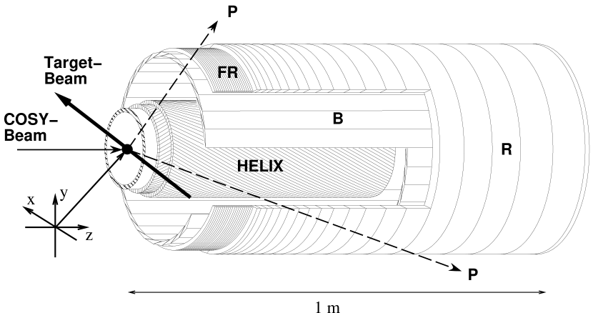
Figure 1: Scheme of the EDDA detector. The outer hodoscope consists of scintillator bars B, scintillator semi-rings R and semi-rings made of scintillating fibers FR. The inner hodoscope HELIX consists of four layers of scintillating fibers helically wound in opposing directions.

For the measurement of spin observables, however, a polarized atomic beam target shall be used. The interaction region of such a target is far from being pointlike. The polarized hydrogen beam has a finite diameter of about 12 mm (FWHM). It is superimposed on a background of unpolarized hydrogen atoms which are due to the residual gas in the beam pipe vacuum. Therefore, a second inner detector shell is required to provide an appropriate vertex reconstruction.

The inner detector shell (HELIX) is a cylindrical hodoscope consisting of four layers of 2.5 mm diameter plastic scintillating fibers which are helically wound in opposing directions so that coincidence of hits in the lefthanded and righthanded helices gives the point at which the ejectile traversed the hodoscope. The 640 scintillating fibers are connected to 16-channel multianode photomultipliers and read out individually using the LeCroy proportional chamber operation system PCOS III. A detailed description of the helical fiber detector can be found in Altmeier et al. (1999). Its purpose is (i) vertex reconstruction of elastic proton-proton scattering events in conjunction with the outer shell, (ii) background suppression of scattering events from the background of unpolarized hydrogen atoms surrounding the polarized hydrogen beam and (iii) improved angular resolution. Combined with the spatial resolution of the outer detector shell, the helix fiber detector provides for vertex reconstruction with a FWHM resolution of 1.3 mm in the x- and y-direction and 0.9 mm in the z-direction. Using a fit of the vertex and scattering angles with constraints imposed by $pp$ elastic scattering kinematics the resulting polar and azimuthal angular resolutions are about 0.3^∘ and 1.3^∘ FWHM.

2.3 Polarized Atomic Hydrogen Beam Target

The polarized atomic hydrogen beam target Eversheim et al. (1997) is shown in Fig. 2. Hydrogen atoms with nuclear polarization are prepared in an atomic-beam source with dissociator, cooled nozzle, permanent sixpole magnets and RF-transition unit. The design of the atomic beam target had to meet constraints imposed by the EDDA experiment. First, the space close to the interaction region is limited: target components must be outside the angular acceptance of the EDDA detector. This dictates a rather large distance of about 30 cm between the second sixpole magnet and the interaction region. Second, in view of the closed orbit distortions in COSY only weak guide fields are allowed such that only one pure hyperfine state can be used. Third, the COSY beam width at injection and the change of the horizontal beam position during acceleration makes the use of a storage cell (typical apertures 10 mm x 10 mm) unfavorable. Reducing the beam width with beam scrapers, and thus the injected beam current would at least partly offset the benefit of higher target densities and lead to increased background.

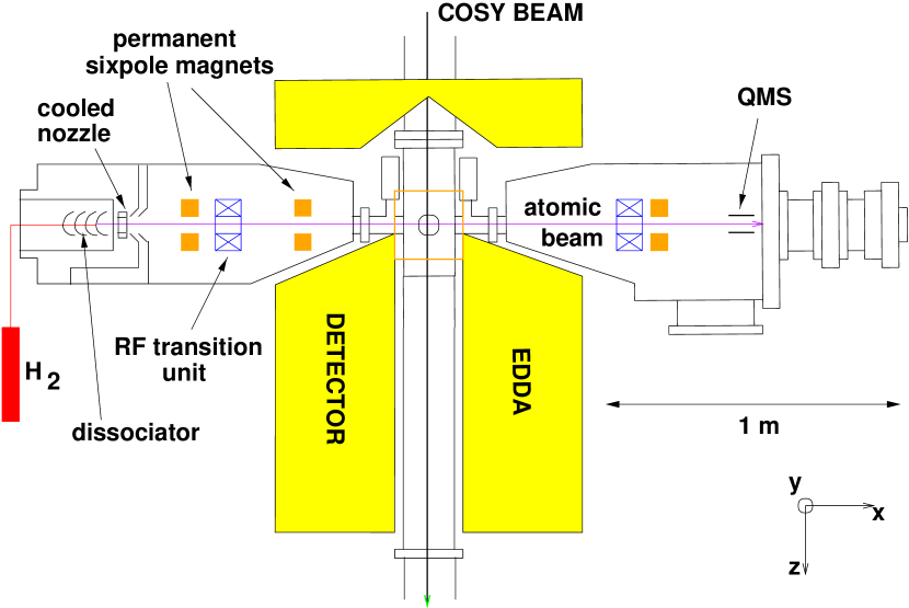
Figure 2: Scheme of the polarized atomic hydrogen beam target.

In the dissociator, hydrogen is dissociated in an inductively coupled 350 W RF-discharge and passes through an aluminum nozzle cooled to about 30 K and a skimmer. About $5\cdot 10^{16}$ hydrogen atoms per second are produced. For the differential pumping a turbomolecular pump of 600 liter/s is used in the first vacuum chamber between nozzle and skimmer and four turbomolecular pumps of 1000 liter/s in the subsequent vacuum chambers. In addition, a cryopump with a pumping speed of about 2300 liter/s is installed in the second sixpole vacuum chamber. In the beam dump turbomolecular pumps of 360 and 600 liter/s and a cryopump of 1000 liter/s are installed. The comparable low temperature of the nozzle leads to a decreased velocity (most probable velocity 1.3 km/s) of the atomic beam and thus an increased target thickness. The atomic beam target is usually operated at 0.5 mbar liter/s hydrogen flow. A small amount of oxygen flow is mixed into the hydrogen flow yielding a thin layer of H₂O-molecules in the region of the cooled nozzle. Thus, the recombination of hydrogen atoms by the cooled nozzle is minimized resulting in an increased target density.

The atomic beam source selects hydrogen atoms in a pure hyperfine state ($m_{j}$=$+1/2$, $m_{I}$=$+1/2$), in order to achieve a high polarization in a weak magnetic holding field. Here, $m_{j}$ and $m_{I}$ are the magnetic quantum numbers of the electron and proton spins, respectively. Hydrogen atoms in the $m_{j}$=$+1/2$ state are focused by the sixpole magnets while those in the $m_{j}$=$-1/2$ state are defocused. The first sixpole magnet removes the two hyperfine states with $m_{j}$=$-1/2$ and the Abragam-Winter RF-transition unit induces an intermediate field transition (IF-transition) to a depopulated hyperfine state, ($m_{j}$=$+1/2$, $m_{I}$=$-1/2$)$\rightarrow$ ($m_{j}$=$-1/2$, $m_{I}$=$+1/2$), which is removed by the subsequent sixpole magnet.

Figure 3: (a) Elastic proton-proton scattering rates to the left and right of the detector and (b) the derived polarization profile as a function of the longitudinal vertex position $z_{v}$ measured with vertical target polarization at $T_{lab}{=}793$ MeV. The polarized atomic hydrogen beam stands out at $z_{v}{=}0$ on an unpolarized background of the residual hydrogen gas in the beam pipe vacuum. The dashed lines indicate the $z_{v}$ vertex cut [-15,+20] mm. The decreasing number of events at $z_{v}{<}-15$ mm is due to the decreasing detector acceptance.

In Fig. 3 typical intensity and polarization distributions are shown as a function of the longitudinal position $z_{v}$. The plot shows the elastic proton-proton scattering rates to the left and right of the detector (a) and the derived polarization (b). The polarized atomic hydrogen beam stands out at $z=0$ on an unpolarized background which is due to the residual hydrogen gas in the beam pipe vacuum. Polarizations of about 90 % are deduced when the unpolarized background is subtracted. The atomic beam width (FWHM) is about 12 mm at the intersection with the COSY beam. A guide field in the interaction region of 1.0 mT pointing up or down was used to align the target spins in the vertical direction. The decrease in rate below $z{<}{-}15$ mm is due to the acceptance of the EDDA hardware trigger. Including the unpolarized background, the effective polarization is about 73% for a $z$-vertex cut [-15 mm, +20 mm] and the effective target thickness is 1.8$\cdot$10¹¹ atoms/cm². The background of unpolarized hydrogen depends on the quality of the COSY vacuum. Therefore, in addition to the standard ion getter pumps, titanium sublimation pumps are switched on. Then, the resulting vacuum in the region of the EDDA-target is $<1\cdot 10^{-9}$ mbar without and about $1\cdot 10^{-8}$ mbar with hydrogen beam target.

The atomic beam profile in $y$-direction has been measured at a fixed flattop energy (796 MeV) by sweeping the COSY beam by steerer magnets across the target and measuring the vertex distribution of elastic proton-proton scattering events. The target density distribution was deduced by fitting a Gaussian distribution for the polarized atomic beam plus a constant unpolarized hydrogen background. The finite width of the COSY beam and the detector resolution function were taken into account by an appropriate folding of the distributions. The resulting atomic beam width (FWHM) in $y$-direction of about 12 mm compares well with the corresponding width in $z$-direction. Similarly, the polarization profile in $y$-direction which was deduced from the measured left-right asymmetries compares well with the corresponding profile in $z$-direction.

Due to the background of unpolarized hydrogen atoms the effective polarization depends on the overlap of the COSY beam with the polarized atomic beam. Fortunately, variations of the vertical position and width of the COSY beam during the acceleration are very small, see Figs. 5 and 6. In addition, the COSY beam is much smaller than the polarized atomic beam. Therefore, the effective target polarization is practically constant during the acceleration and deceleration.

In the beam dump the polarization of the atomic beam is continuously monitored using an additional RF-transition unit and a permanent sixpole magnet as Breit-Rabi polarimeter.

2.4 Magnetic Guide Field

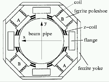
Figure 4: Magnet for the guide field of the target polarization. Magnetic guide fields of 1.0 mT in $\pm x$- and $\pm y$-direction are produced near the beam axis by linear superposition of A- and B-fields.

The magnet for the guide field of the target polarization is shown schematically in Fig. 4. It consists of a ferrite yoke and ferrite pole shoes located external to the vacuum chamber. The magnetic fields in $x$- and $y$-direction are produced by superposing two fields of equal strength along the azimuthal directions 45^∘ and 135^∘. The earth magnetic field is shielded to a high degree by the ferrite yoke. The residual magnetic field is compensated by a small correction field using the magnet for the guide field. The currents for the magnetic guide fields and the field corrections are controlled by a personal computer. The direction of the target polarization was changed from cycle to cycle by changing the direction of the guide field from $+x$ to $-x$ and $+y$ to $-y$. Using a flux gate probe the resulting field distributions were measured as a function of $x$, $y$ and $z$. These measurements proved a high magnetic field homogeneity across the fiducial vertex volume.

The strength of the magnetic field was chosen to be 1.0 mT. This value is sufficiently large compared to the field distortion produced by the circulating beam particles at the interaction point. On the other hand, the resulting distortion of the closed orbit is sufficiently small. It can be calculated using the COSY lattice parameters at the target point. For beam momenta between 1.0 and 3.3 GeV/c the resulting angle kick varies between 60 and 18 $\mu$rad yielding a horizontal closed orbit shift $\Delta x$ between 51 and 16 $\mu$m for guide fields along the $y$-direction. Similar values are obtained for the vertical closed orbit distortions. The closed orbit distortions deduced from the vertex reconstruction of the data are in good agreement with these estimates.

2.5 COSY Beam

The ramping speed of COSY was changed from the usual value 1.1 (GeV/c)/s to 0.55 (GeV)/s and data were taken during acceleration as well as deceleration of the COSY beam. The time period of one cycle was about 15 s. With an average of 2.8$\cdot$10¹⁰ protons in the ring, luminosities of about 8$\cdot$10²⁷cm^-2s^-1 were achieved and accumulated to an integrated luminosity of $\sim$10³⁴ cm^-2. The beam parameters were continuously measured during the acceleration ramp. The beam momentum is derived from the RF of the cavity and the circumference of the closed orbit with an uncertainty of 0.25 to 2.0 MeV/c for the lowest and highest momentum, respectively.

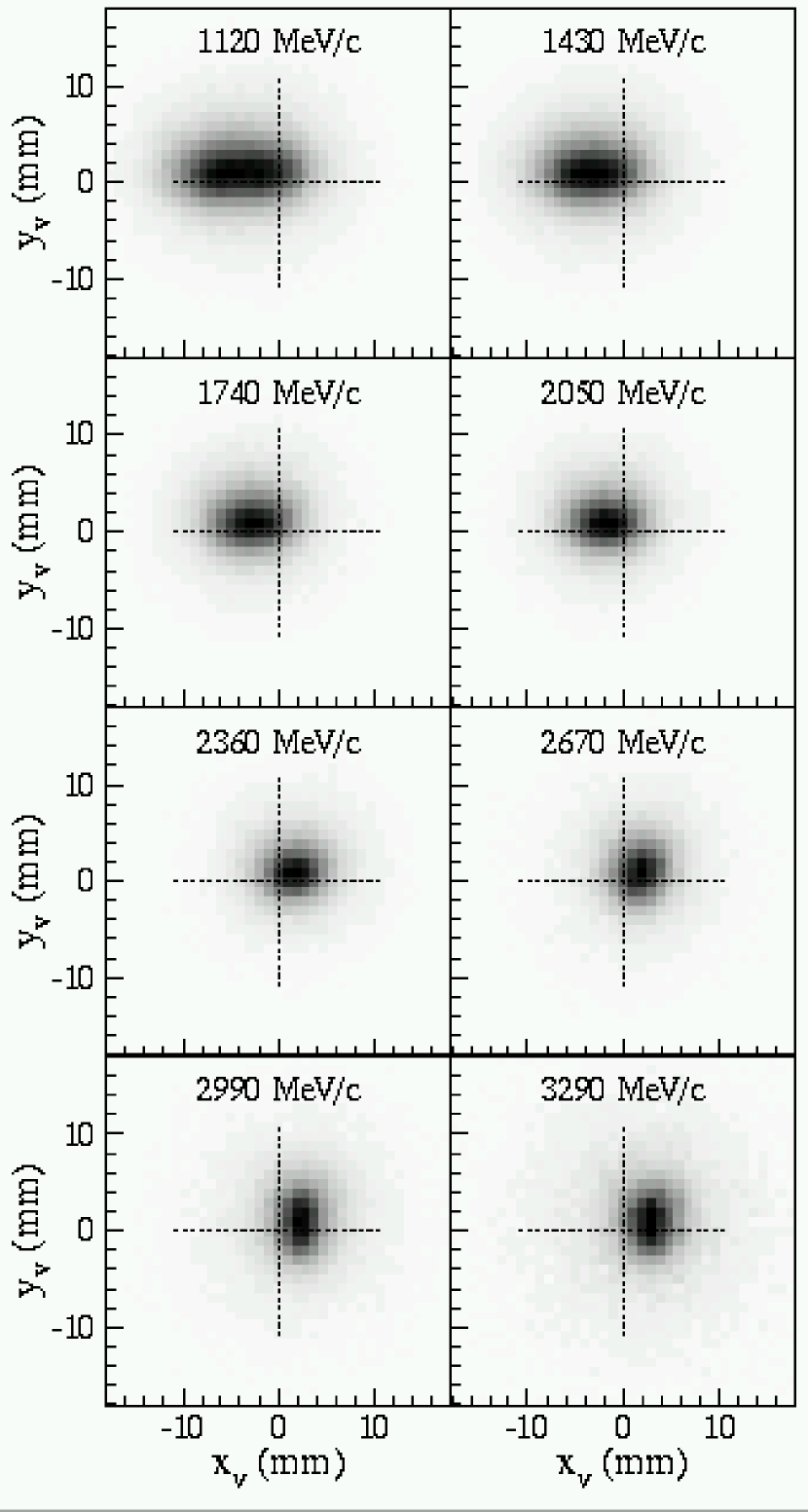
Figure 5: Vertex distributions in the $(x,y)$-plane for the running period November 98.

The $x$-$y$ density distributions of the COSY beam can be deduced from the measured vertex distributions. Thus, beam position and width can be reconstructed as a function of the beam momentum. Typical vertex distributions are shown in Fig. 5 in the form of two-dimensional scatter plots. Since the polarized atomic beam target is directed in $x$-direction and its width in $y$-direction is rather large these distributions resemble approximately the COSY beam density. Interestingly, the horizontal beam position and width change slowly during the acceleration and deceleration whereas the vertical beam position and width stay nearly constant. This behaviour can be seen more clearly by plotting the mean values and $\bar{x}$, $\bar{y}$ and the FWHM-widths $\Delta x{=}2.35\sigma_{x}$, $\Delta y{=}2.35\sigma_{y}$ as a function of the COSY cycle time $t$, see Fig. 6.

The deviations from the nominal beam position $\bar{x}=0$ and $\bar{y}=0$ indicate (i) misalignments of the detector and (ii) closed orbit distortions of the COSY beam which are caused by small deviations from the nominal magnetic dipole fields in the accelerator ring. In all three running periods the horizontal deviations $\bar{x}$ vary systematically as a function of beam momentum between at most -5 mm and +2 mm. Vertically, a small but constant offset of $\bar{y}\approx+1.5$ mm was observed, see Fig. 6.

Figure 6: Beam position (thick lines) and beam width (FWHM, thin lines) in x- and y-direction as a function of the accelerator time for three running periods. The horizontal lines mark the start of data taking in the acceleration ramp, the beginning of the flattop momentum region and the beginning of the deceleration ramp.

Variations of the horizontal and vertical beam widths $\sigma_{x}$ and $\sigma_{y}$ are expected since the adiabatic damping causes a $1/p_{lab}$ dependence of the beam emittances $\epsilon_{x}$ and $\epsilon_{y}$. In addition the optics of the accelerator ring, i.e. the amplitude functions $\beta_{x}$ and $\beta_{y}$ may depend on $p_{lab}$. The equations for $\sigma_{x}$ and $\sigma_{y}$ read

$$\sigma_{x}=\sqrt{\epsilon_{x}\beta_{x}},\;\;\;\sigma_{y}=\sqrt{\epsilon_{y}\beta_{y}}.$$ (1)

If the amplitude functions $\beta_{x}$ and $\beta_{y}$ are constant a $1/\sqrt{p_{lab}}$ dependence of the beam widths is expected. However, in the chosen mode of operation $\beta_{x}$ was decreasing and $\beta_{y}$ increasing with $p_{lab}$. As a consequence, the horizontal beam width $\sigma_{x}$ was rather strongly decreasing with $p_{lab}$ whereas the vertical beam width $\sigma_{y}$ was nearly constant.

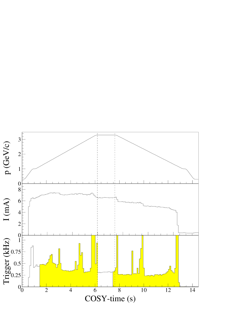
Figure 7: Typical COSY machine cycle: beam momentum $p{=}p_{lab}$, beam current $I$ and trigger rate as a function of the COSY cycle time. The dashed vertical lines denote the flattop region.

The approximate constancy of the vertical beam profile is of great importance for the effective target polarization which depends on the overlap between beam and target. The vertical width of the target beam (12 mm, FWHM) is about a factor two larger than the vertical width of the COSY beam and the variations of the vertical beam position and beam width during the acceleration and deceleration are negligibly small with respect to the vertical width of the target beam.

3 Data Acquisition and Processing

3.1 Measuring Cycle

Measurements of the excitation functions $A_{N}$($p_{lab}$, $\Theta_{c.m.}$) were performed in cycles of about 15 s duration with data acquisition extending over the acceleration, the flattop at 3.3 GeV/c, and the deceleration as well. A typical machine cycle is shown in Fig. 7. The beam current is nearly constant during the acceleration and slowly decreasing during the deceleration. The trigger rate and the dead time show huge excursions at certain COSY-times which are caused by increased background due to beam losses. Fortunately, these excursions occured at different COSY-times in the three running periods. The direction of the target polarization was changed cyclewise yielding the sequence $+x$, $-x$, $+y$, $-y$. The target was operating very stable and with constant polarization during subsequent acceleration cycles.

3.2 Identification of Elastic pp Events

The outer detector shell provides a fast and efficient trigger based on (i) the coplanarity and (ii) the kinematic correlation of two-prong events that fulfill the kinematics of elastic proton-proton scattering. Elastic proton-proton scattering events are identified by coplanarity with the beam axis

$$|\varphi_{1}-\varphi_{2}|=180^{\circ}$$ (2)

and kinematic correlation

$$\tan\Theta_{1}\tan\Theta_{2}=\frac{2m_{p}}{2m_{p}+T_{lab}}.$$ (3)

Here, $\Theta$ and $\varphi$ are the polar and azimuthal angles in the lab system, $m_{p}$ is the mass of the proton and $T_{lab}$ its laboratory kinetic energy.

Figure 8: Definition of the kinematic deficit $\alpha$ in the c.m. system.

In contrast to measurements of d$\sigma$/d$\Omega$ with CH₂ fiber targets Albers et al. (1997, 2004) the data rate with an atomic beam target was rather low. Therefore, only the coplanar trigger, i.e. the coincidence of two opposite bars, was applied in the on-line trigger for the analyzing power measurements. The kinematic correlation was established in the off-line analysis.

The signature of an elastic event can be represented by one variable, the so-called kinematic deficit $\alpha$, which gives the spatial angle deviation from back-to-back scattering in the c.m.-system (see Fig. 8). The kinematic deficit $\alpha$ can be determined in the off-line analysis by transforming the trajectories of two coincident particles into the c.m.-system assuming the kinematics of elastic proton-proton scattering. The resulting distributions of the spatial angle $\alpha$ start with zero at $\alpha=0^{\circ}$ and show a narrow peak followed by a long tail, see Fig. 9. The finite width of the elastic peak is due to the effects of small angle scattering and the finite angle resolution of the detector. Elastic $pp$ scattering events can be identified using a momentum dependent cut,

$$\alpha<\alpha_{cut},\;\;\;\alpha_{cut}=[11.0-p/(1\;{\rm GeV/c})]^{\circ}.$$ (4)

Figure 9: Measured distributions of the kinematic deficit $\alpha$ at two beam momenta. The vertical lines show the momentum dependent cut for the selection of elastic pp scattering events.

3.3 Vertex Reconstruction

In the off-line analysis the coordinates of two kinematically correlated trajectories are deduced from the hit pattern in the inner and outer detector shells. The vertex is determined geometrically by the subroutine FINDTRACKS as the point of closest approach of two outgoing trajectories in the target region.

In order to improve the vertex reconstruction the data are reanalyzed in a kinematic vertex fit with the kinematic constraints of elastic proton-proton scattering. The kinematic fit of two proton trajectories to the hit pattern of an event under the constraint of elastic scattering kinematics is used to define a $\chi^{2}$ criterion for a further event selection. This method yields for instance at $T_{lab}{=}1500$ MeV and $\Theta_{c.m.}{=}40^{\circ}$ a vertex resolution with $\sigma_{x}{=}0.6$ mm, $\sigma_{y}{=}0.6$ mm and $\sigma_{z}{=}0.4$ mm and an angle resolution with $\sigma_{\Theta_{c.m.}}{=}0.6^{\circ}$ and $\sigma_{\varphi}{=}0.8^{\circ}$.

The $\chi^{2}$-distribution is equivalent to the $\alpha$-distribution with respect to the identification of elastic scattering events. The upper part of Fig. 10 shows an example of a $\chi^{2}$-distribution from a kinematic vertex fit at $p_{lab}{=}2280$ MeV/c and $\Theta_{c.m.}{=}89^{\circ}$. The dashed line is an extrapolation in order to estimate an upper limit of the background contribution. A momentum dependent cut

$$\chi^{2}<\chi^{2}_{cut},\;\;\;\chi^{2}_{cut}=28.0-5.5p/{\rm GeV/c}$$ (5)

was chosen as final selection criterion for an elastic $pp$ scattering event, see vertical lines in Fig. 10.

3.4 Background

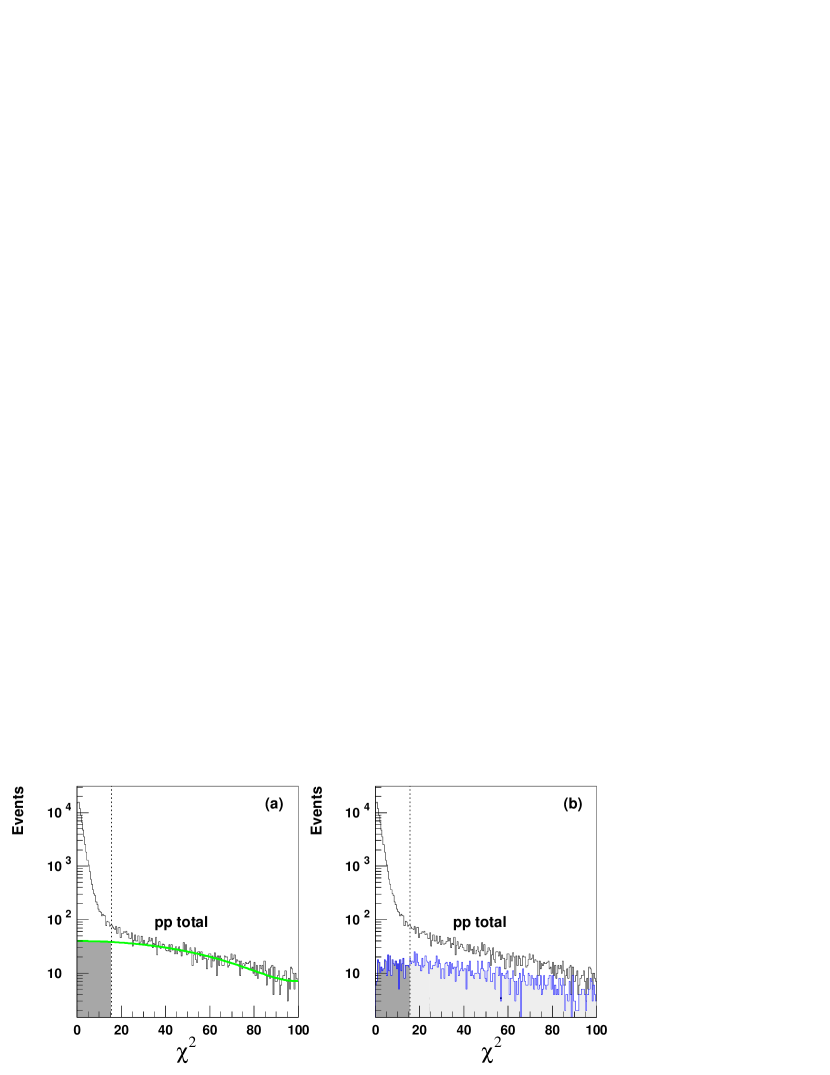
Figure 10: Upper part: Example of a $\chi^{2}$-distribution. The dashed line is an extrapolation from $\chi^{2}{>}30$ to zero. The vertical line shows the cut for the selection of elastic pp scattering events. Lower part: Monte Carlo simulation of a $\chi^{2}$-distribution at 2.3 GeV/c. (a) Extrapolation from $\chi^{2}{>}30$ to zero. (b) The inelastic background contribution (lower histogram)

The reduction of background takes advantage of the reconstructed vertex and the multiplicity patterns in both detector layers. Narrow cuts were applied to the hit pattern and to the vertex coordinate $z$ in COSY beam direction, [-15 mm, +20 mm], a wider one in the $x,y$ plane around the beam profile (3$\sigma$ limits) along an ellipse following the slow drift and shape variation of the COSY beam during acceleration, see Figs. 5,6. The remaining inelastic background was estimated guided by Monte Carlo simulations of elastic and inelastic $pp$ interactions. For the simulation of the hadronic reactions the code MICRES Ackerstaff et al. (2002) was used.

Monte Carlo simulations show that the long tail of the $\alpha$- and $\chi^{2}$-distributions is mainly due to misidentified elastic scattering events suffering from a secondary reaction in the beam pipe and the inner detector shell. This is in accordance with the fact that events with $\alpha{>}\alpha_{cut}$ ($\chi^{2}{>}\chi_{cut}^{2}$) show analyzing powers very similar to the elastic scattering. Therefore, extrapolating the $\alpha$- and $\chi^{2}$-distributions from large $\chi^{2}$-values to zero as shown in Fig. 10 overestimates the inelastic background under the elastic peak. This background of inelastic reactions like $pp\rightarrow pp\pi^{0}$, $pp\rightarrow pn\pi^{+}$, $pp\rightarrow pp\pi^{+}\pi^{-}$, $pp\rightarrow pp\pi^{0}\pi^{0}$, and $pp\rightarrow pn\pi^{+}\pi^{0}$ is rather small. It was estimated to be mostly $\leq$ 2% and only at highest energies near $\Theta_{c.m.}{=}90^{\circ}$ up to 4.5%.

3.5 Determination of Analyzing Power

Figure 11: Definition of four detector sectors for the determination of the analyzing power with, looking along the beam axis, L (Left), R (Right), B (Bottom) and T (Top). The azimuthal angle $\varphi$ gives the rotation of the scattering plane and it’s coordinate system $(S,N,L)$ with respect to the fixed coordinate system $(x,y,z)$ of beam and target. The sectors with $75^{\circ}{<}\varphi{<}105^{\circ}$ and $255^{\circ}{<}\varphi{<}285^{\circ}$ are not used since the angle reconstruction is affected by the readout of the half rings, see Fig. 1.

We denote the target polarization by $\vec{Q}{=}(Q_{x},Q_{y},Q_{z})$. In order to eliminate systematic errors the direction of the target polarization was changed from cycle to cycle between $\pm x$ and $\pm y$,

$$+x : \vec{Q}=(+|\vec{Q}|,0,0),\;\;Q^{+}_{x}=+|\vec{Q}|$$

$$-x : \vec{Q}=(-|\vec{Q}|,0,0),\;\;Q^{-}_{x}=-|\vec{Q}|$$

$$+y : \vec{Q}=(0,+|\vec{Q}|,0),\;\;Q^{+}_{y}=+|\vec{Q}|$$

$$-y : \vec{Q}=(0,-|\vec{Q}|,0),\;\;Q^{-}_{y}=-|\vec{Q}|.$$ (6)

The polarized differential cross section may be written

$$\frac{{\rm d}\sigma}{{\rm d}\Omega}=\frac{{\rm d}\sigma_{0}}{{\rm d}\Omega}[1+A_{N}(Q_{y}\cos{\varphi}-Q_{x}\sin{\varphi})].$$ (7)

Here, ${\rm d}\sigma_{0}/{\rm d}\Omega$ is the unpolarized differential cross section, $A_{N}$ the analyzing power with respect to a polarization component in the direction N normal to the scattering plane. The azimuthal angle $\varphi$ gives the rotation of the scattering plane and it’s coordinate system $(S,N,L)$ with respect to the fixed coordinate system (x,y,z) of beam and target, see Fig. 11.

In order to eliminate false asymmetries arising from differences of the luminosities, efficiencies and solid angles of the detector and from misalignments, the geometric mean method of Ohlsen and Keaton Ohlsen (1973) is used. Two sets of cycles with opposite polarizations, e.g. $Q^{+}_{y}$ and $Q^{-}_{y}$, were combined to apply a “proper spin flip” correction for false asymmetries. Indicating the number of events obtained simultaneously for the detector elements in the angle position $(\Theta,\varphi)$ with $N^{+}(\Theta,\varphi)$ for spin up and $N^{-}(\Theta,\varphi)$ for spin down we define

$$L=\sqrt{N^{+}(\Theta,\varphi)N^{-}(\Theta,\varphi+\pi)}$$ (8)

and

$$R=\sqrt{N^{-}(\Theta,\varphi)N^{+}(\Theta,\varphi+\pi)}$$ (9)

to calculate the left–right asymmetry

$$\epsilon_{LR}=\frac{L-R}{L+R}$$ (10)

for a pair of detector elements in the azimuthal positions $\varphi$ and $\varphi+\pi$ with $-\pi/2<\varphi<+\pi/2$. The analyzing power $A_{N}(\Theta)$ is deduced as weighted mean over all $\varphi$-bins using

$$A_{N}(\Theta)=\frac{1}{\cos\varphi}\frac{\epsilon_{LR}(\Theta,\varphi)}{Q_{y}},\;\;\;-\pi/2<\varphi<\pi/2.$$ (11)

Here, the moduli of the target polarizations are assumed to be equal, $|Q^{+}_{y}|=|Q^{-}_{y}|=|\vec{Q}|$.

Similarly the runs with $Q^{\pm}_{x}$ were used to deduce $A_{N}$ from the bottom–top asymmetries $\epsilon_{BT}$ for a pair of detector elements in the azimuthal positions $\varphi$ and $\varphi+\pi$ with $-\pi<\varphi<0$,

$$A_{N}(\Theta)=-\frac{1}{\sin\varphi}\frac{\epsilon_{BT}(\Theta,\varphi)}{Q_{x}},\;\;\;-\pi<\varphi<0,$$ (12)

assuming $|Q^{+}_{x}|=|Q^{-}_{x}|=|\vec{Q}|$. The terms Left (L), Right (R), Bottom (B) and Top (T) always refer to the scattered proton detected at forward scattering angles with $\Theta_{c.m.}\leq 90^{\circ}$.

This method eliminates exactly all false asymmetries that means asymmetries which would still be observed with no target polarization. Thus, the result is independent of relative detector efficiencies and solid angles, since they do not vary with time over the period of two adjacent cycles. It is also independent of time fluctuations in the beam current or target density as well as differences in the integrated charge and target thickness.

Misalignments of the beam axis with respect to the detector axis yield small deviations from the nominal scattering angles $\Theta_{c.m.}$ and small variations of the solid angles. These misalignments depend on the closed orbit distortions during the beam acceleration and deceleration. Again, there is exact cancellation of false asymmetries due to deviations of the solid angles. But since the analyzing power $A_{N}$ depends on the scattering angle $\Theta_{c.m.}$ the determination of the effective scattering angle becomes an important experimental task. Fortunately, the EDDA detector allows to reconstruct the scattering angle $\Theta$ for each event with high accuracy. Thus, systematic errors from these deviations are also avoided.

The geometric mean correction method assumes the moduli of the target polarizations $Q^{\pm}_{y}$ and $Q^{\pm}_{x}$ to be equal. This assumption is very well fulfilled since the polarization vector follows adiabatically the direction of the magnetic guide field and the spin flip is realized by flipping the direction of the guide field. Small deviations that may occur cause negligible effects. For instance deviations with $|Q^{+}_{y}|-|Q^{-}_{y}|\leq 0.02$ influence $A_{N}$ by at most $7\cdot 10^{-5}$.

3.6 Absolute Target Polarization

Figure 12: Angular distribution at 1379 MeV/c (730 MeV) in comparison to the LAMPF data McNaughton et al. (1990) which were used for the absolute normalization. The momentum bin width of the EDDA data is here 60 MeV/c.

The absolute values of the effective target polarizations $Q_{x}$ and $Q_{y}$ are established in each running period for one momentum bin $\Delta p_{lab}$ = 60 MeV/c around the energy $T_{lab}=730$ MeV ($p_{lab}=1379$ MeV/c). The absolute values of $Q_{x}$ and $Q_{y}$ are deduced as weighted means over all $\varphi$-bins from the measured asymmetries,

$$Q_{x}=-\frac{\epsilon_{BT}(\Theta,\varphi)}{\sin\varphi A_{N}(\Theta)},\;\;\;-\pi<\varphi<0,$$ (13)

$$Q_{y}=\frac{\epsilon_{LR}(\Theta,\varphi)}{\cos\varphi A_{N}(\Theta)},\;\;\;-\pi/2<\varphi<\pi/2.$$ (14)

The precise angular distribution $A_{N}(\Theta)$ from McNaughton et al. McNaughton et al. (1990) with an absolute normalization error of 1 % is taken as reference value, see Fig. 12. Taking the relative errors of the data into account the overall normalization error of the present data is 1.2 %. The effective target polarization is constant during the acceleration and deceleration since the overlap between COSY beam and polarized atomic beam target is constant. The observed small variations of the vertical beam width (see Fig. 6) cause variations of the effective target polarization of less than 0.3 %.

3.7 Effective Target Polarization at Forward Angles

The influence of the restrictions by the detector acceptance has been studied separately. It yields small modifications of the effective target polarization at low energies and small scattering angles. There, events with negative $z$-values of the vertex point cannot be detected if the recoil protons are outside the detector acceptance. As a consequence the effective target volume is reduced in the $z$-direction from $[-15\;{\rm mm},+20\;{\rm mm}]$ to $[z_{min},+20\;{\rm mm}]$ and the average polarization within this reduced volume, subsequently called the effective polarization, differs from the full-acceptance value. This modification is due to the background of unpolarized hydrogen atoms, see Fig. 3. It can be studied in a systematic way by artificially restricting the vertex range in $z$-direction for all $(\Theta_{c.m.},p_{lab})$-bins with full acceptance and deducing the weighted mean of the resulting asymmetry ratios $\epsilon([z_{min},+20\;{\rm mm}])/\epsilon([-15\;{\rm mm},+20\;{\rm mm}])$ as a function of $z_{min}$. These asymmetry ratios can directly be used as correction factors of the effective target polarization at low energies and small scattering angles where the $z$-range is restricted.

4 Results

4.1 Consistency Checks

The COSY beam changes its shape and position during acceleration and deceleration, though very reproducible in each cycle. Prior to merging all data in one final set it was necessary to perform consistency checks on subsets obtained under different conditions of polarization and acceleration cycle. They demonstrated that the guide field is properly aligned to the detector coordinates (x,y), and that during acceleration and deceleration the same analyzing powers are obtained Altmeier et al. (2000). This implies that vertex reconstruction and proper flip elimination of false asymmetries work well. A comparison of analyzing powers $A_{N}$ at $\Theta_{c.m.}{=}60^{\circ}$ acquired during the running periods June 98, November 98 and May 99 is shown in Fig. 13. Since all data are compatible they are combined in one set. Altogether 3.1$\cdot$10⁷ elastic scattering events were collected.

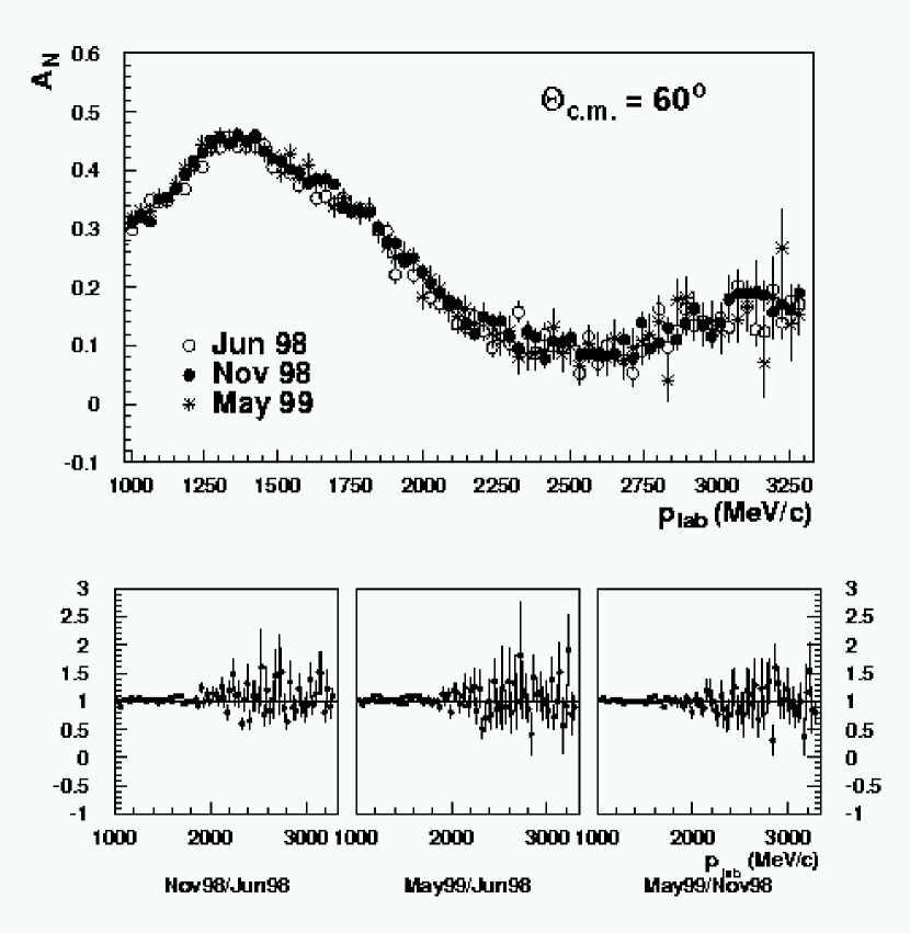
Figure 13: Comparison of analyzing powers $A_{N}$ at $\Theta_{c.m.}{=}60^{\circ}$ acquired during the running periods June 98, November 98 and May 99.

4.2 Errors

Error estimates for $A_{N}$ include contributions from the maximum deviations between data subsets ($\leq$ 2.1%), and the impact of the background on the asymmetry ($\leq$ 0.008). Errors due to closed orbit distortions by the variation of the magnetic guide field with changes of the proton beam position and angle are negligible, see Sect. 2.4.

Figure 14: Excitation functions of $A_{N}$ from the present work at eight out of 15 c.m. angles in comparison to the phase shift solutions SP00 (dashed curve) and FA00 (solid curve) Arndt et al. (2000). The bin widths are $\Delta p_{lab}{=}30$ MeV/c and $\Delta\Theta_{c.m.}{=}4^{\circ}$. The data at the flattop momentum 3.3 GeV/c exhibit an especially small statistical error.

The overall absolute normalization uncertainty of the excitation functions is $\pm 1.2$ % in the full energy range 0.45–2.5 GeV. It is due to the absolute normalization uncertainty of $\pm 1$ % from the reference data McNaughton et al. (1990) and the relative errors of the data at 730 MeV. This systematic uncertainty is not included in Figs. 14 and 16 and the tables available upon request Dat , and must be applied to all data.

4.3 Excitation Functions

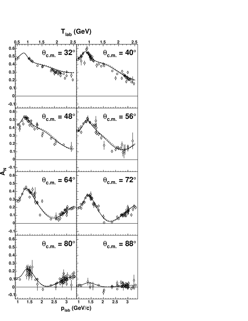
Figure 15: Collection of published data from the data base of Arndt et al. (2000) without EDDA data of Altmeier et al. Altmeier et al. (2000) plotted as excitation functions at eight c.m. angles in comparison to the phase shift solutions SP00 (dashed curve) and FA00 (solid curve) Arndt et al. (2000). $\circ$ SATURNE II Allgower et al. (1999a, b); Ball et al. (1999); Allgower et al. (1998); Arvieux et al. (1997); Perrot et al. (1987), $\triangle$ KEK Kobayashi et al. (1994), $\diamond$ ZGS Parry et al. (1973); Miller et al. (1977); Bell et al. (1980), $\star$ LAMPF McNaughton et al. (1990); Bevington et al. (1978); McNaughton et al. (1982), $\square$ IUCF von Przewoski et al. (1998), $+$ SIN Besset et al. (1980); Berdoz et al. (1983); Aprile et al. (1986).

Excitation functions $A_{N}(p_{lab},\Theta_{c.m.}$) with about 1150 data have been deduced from our experimental results by grouping them into $\Delta\Theta_{c.m.}{=}4^{\circ}$ and $\Delta p_{lab}{=}30$ MeV/c wide bins. They supersede the results of the EDDA Collaboration reported in Altmeier et al. (2000) and are available upon request Dat . Here, excitation functions at eight out of 15 c.m. angles are displayed in Fig. 14.

4.4 Angular Distributions

Figure 16: Angular distributions of $A_{N}$ from the present work at eight out of 77 beam momenta in comparison to the phase shift solutions SP00 (dashed curve) and FA00 (solid curve) Arndt et al. (2000). The bin widths are $\Delta p_{lab}{=}30$ MeV/c and $\Delta\Theta_{c.m.}{=}4^{\circ}$. The data at the flattop momentum 3.3 GeV/c exhibit a small statistical error.

The data can also be presented in the form of angular distributions. In Fig. 16 eight out of 77 angular distributions for $\Delta\Theta_{c.m.}{=}4^{\circ}$ and $\Delta p_{lab}{=}30$ MeV/c wide bins are shown. Again, these data supersede the results of the EDDA Collaboration reported in Altmeier et al. (2000) and are available upon request Dat .

Figure 17: Collection of published data from the data base of Arndt et al. (2000) without EDDA data of Altmeier et al. Altmeier et al. (2000) plotted as angular distributions at eight momenta in comparison to the phase shift solutions SP00 (dashed curve) and FA00 (solid curve) Arndt et al. (2000). $\circ$ SATURNE II Allgower et al. (1999a, b); Ball et al. (1999); Allgower et al. (1998); Arvieux et al. (1997); Perrot et al. (1987), $\triangle$ KEK Kobayashi et al. (1994), $\diamond$ ZGS Parry et al. (1973); Miller et al. (1977); Bell et al. (1980), $\star$ LAMPF McNaughton et al. (1990); Bevington et al. (1978); McNaughton et al. (1982), $\square$ IUCF von Przewoski et al. (1998), $+$ SIN Besset et al. (1980); Berdoz et al. (1983); Aprile et al. (1986).

5 Discussion

5.1 Comparison to other data

Previous $A_{N}$ data were mainly measured at discrete energies. A collection of published data from the SAID data base Arndt et al. (2000) is shown in Figs. 15 and 17. The most recent results in the kinetic energy range 0.8–2.8 GeV are from SATURNE II Allgower et al. (1999a, b); Ball et al. (1999); Allgower et al. (1998); Arvieux et al. (1997). They are in good agreement with the present data. The same holds true for the results from SATURNE II of Perrot et al. Perrot et al. (1987) at the kinetic energies (momenta) 0.874 (1.550), 1.095 (1.804), 1.295 (2.027), 1.596 (2.354), 1.796 (2.568), 2.096 (2.886) and 2.396 GeV (3.200 GeV/c). The ZGS data of Parry et al. Parry et al. (1973) at 1.73 (2.5), 1.97 (2.75), 2.14 (2.93) and 2.44 GeV (3.25 GeV/c) and Miller et al. Miller et al. (1977) at 1.27 (2.0) and 2.21 GeV (3.0 GeV/c) show considerable deviations in the angular distributions.

In the kinetic energy range 0.45–0.8 GeV the world data set exhibits several high precision measurements at discrete energies. The absolute normalization of our $A_{N}$ excitation functions was established at $T_{lab}{=}730$ MeV ($p_{lab}{=}1379$ MeV/c) by taking the precise angular distribution $A_{N}(\Theta)$ of McNaughton et al. McNaughton et al. (1990) as reference value. Our data below and above 730 MeV (1379 MeV/c) are in very good agreement with other precise LAMPF measurements of McNaughton et al. McNaughton et al. (1982) at 643 MeV (1273 MeV/c) and Bevington et al. Bevington et al. (1978) at 787 (1448) and 796 MeV (1459 MeV/c) as well as with precise IUCF measurements of Przewoski et al. von Przewoski et al. (1998) at 448.9 MeV (1022 MeV/c), SIN measurements of Besset et al. Besset et al. (1980), Berdoz et al. Berdoz et al. (1983), Aprile et al. Aprile et al. (1986) between 400 and 600 MeV (954 and 1219 MeV/c) and SATURNE measurements of Allgower et al. Allgower et al. (1999b) at 795 MeV (1457 MeV/c).

5.2 Comparison to Partial-Wave Analyses

After the publication of the first unpolarized differential cross section data from EDDA Albers et al. (1997) the VPI group extended their energy dependent phase shift analysis from 1.6 GeV (2.36 GeV/c) up to 2.5 GeV (3.3 GeV/c) laboratory kinetic energy (beam momentum) with the solution SM97 Arndt et al. (1997). Meanwhile energy dependent phase shift solutions are available with a maximum beam energy (beam momentum) of 3.0 GeV (3.82 GeV/c) Arndt et al. (2000). The solution SP00 includes the recent $A_{N}$ data from IUCF Haeberli et al. (1997); Rathmann et al. (1998); von Przewoski et al. (1998); Lorentz et al. (2000) and Saclay Allgower et al. (1999a, b). The recent $A_{N}$ data from EDDA Altmeier et al. (2000) are included in the solution FA00.

The comparison of the present data to the phase shift solution FA00 Arndt et al. (2000) yields agreement in the size and the general angle and momentum dependence of the excitation functions and angular distributions, see Figs. 14 and 16. Small systematic deviations can be seen in the excitation functions, in particular for momenta from 1.8 – 2.5 GeV/c. As can be seen in Fig. 14 the difference between the solutions FA00 and SP00 is small and the systematic deviations in the momentum range 1800 – 2500 MeV/c remain. It is interesting to note that the analyzing power data are slightly negative in the region around $p_{lab}{=}2.0$ GeV/c and $\Theta_{c.m.}{=}80^{\circ}$ whereas the the phase shift solutions remain positive. This observation is in agreement with previous Saclay data Perrot et al. (1987) in that region.

Including the EDDA data into the solution FA00 turned out that the agreement of the phase shift solution with the new $A_{N}$ data was slightly improved. The spin triplet phases, e.g. those of the ${}^{3}F_{2}$ partial wave experienced significant changes. This is due to the fact, that the analyzing power times differential cross section is equal to the real part $Re(a^{\star}\cdot e)$, where the invariant amplitudes $a$ and $e$ Lechanoine-LeLuc and Lehar (1993); Bystricky et al. (1978) include only triplet partial waves.

5.3 Sensitivity to narrow resonances

All excitation functions of the analyzing powers show a smooth dependence on beam momentum. There is no evidence for narrow resonances.

A previous internal target experiment at KEK Kobayashi et al. (1994) observed two narrow structures in the excitation function of the analyzing power $A_{N}$ at a laboratory kinetic energy near 632 MeV corresponding to $\sqrt{s}=2.17$ GeV. Those measurements were performed using a polarized proton beam in the KEK ring and a 30 $\mu$m thick polyethylene fiber target. The outgoing protons were detected at a fixed backward angle of 68^∘ in coincidence with a forward detector. The corresponding c.m. angle near 632 MeV was 38.4^∘. In the present work all excitation functions including those near 38^∘ are smooth. Our result is in agreement with the measurements of Beurty et al. Beurtey et al. (1992).

The fact that $A_{N}d\sigma/d\Omega=Re(a^{\star}\cdot e)$ includes only triplet partial waves implies that the excitation functions for $A_{N}$ are more sensitive to resonant excursions in triplet than to those in singlet partial waves. However, the excitation functions measured here exhibit no evidence for energy–dependent structures. It should be noted that also the excitation functions of $d\sigma/d\Omega$ did not show any evidence for energy–dependent structures Albers et al. (1997, 2004). A more detailed discussion of sensitivities to and upper limits for such structures will be given in a forthcoming paper.

6 Conclusions

In conclusion, we report on the first measurement of analyzing power excitation functions $A_{N}(p_{lab},\Theta_{c.m.})$ in the laboratory momentum range 1.0–3.3 GeV/c and the c.m. angle range $30^{\circ}$–$90^{\circ}$ for proton-proton scattering during acceleration and deceleration in a synchrotron. The data provide a new polarization standard and can be used for calibration purposes in the full energy range 0.45–2.5 GeV. The excitation functions agree with fixed energy data and close the gaps in between with data of high precision and consistency. The phase shift analysis including our data yields a global phase shift solution for $T_{lab}$ up to 2.5 GeV (FA00) showing distinct deviations from previous phase shift solutions that occur mainly in the spin triplet phases. Further progress can be expected from the new excitation functions of the spin correlation parameters $A_{NN}$, $A_{SS}$ and $A_{SL}$ measured by the EDDA experiment.

References

- Albers et al. [1997] D. Albers et al. (EDDA), Phys. Rev. Lett. 78, 1652 (1997).
- Altmeier et al. [2000] M. Altmeier et al. (EDDA), Phys. Rev. Lett. 85, 1819 (2000).
- Albers et al. [2004] D. Albers et al. (EDDA), Eur. Phys. J. Axx, yy (2004).
- Maier [1987] R. Maier, Nucl. Instr. and Meth. A390, 1 (1987).
- Bourrely et al. [1980] C. Bourrely, J. Soffer, and E. Leader, Phys. Rept. 59, 95 (1980).
- Bystricky et al. [1978] J. Bystricky, F. Lehar, and P. Winternitz, J. Phys. (Paris) 39, 1 (1978).
- Lechanoine-LeLuc and Lehar [1993] C. Lechanoine-LeLuc and F. Lehar, Rev. Mod. Phys. 65 (1993).
- Stoks et al. [1993] V. G. J. Stoks, R. A. M. Klomp, M. C. M. Rentmeester, and J. J. de Swart, Phys. Rev. C48, 792 (1993).
- Bystricky et al. [1987] J. Bystricky, C. Lechanoine-LeLuc, and F. Lehar, J. Phys. (Paris) 48, 199 (1987).
- Bystricky et al. [1990] J. Bystricky, C. Lechanoine-LeLuc, and F. Lehar, J. Phys. (Paris) 51, 2747 (1990).
- Nagata et al. [1996] J. Nagata, H. Yoshino, and M. Matsuda, Prog. Theor. Phys. 95, 691 (1996).
- Arndt et al. [1994] R. A. Arndt, I. I. Strakovskii, and R. L. Workman, Phys. Rev. C50, 2731 (1994).
- Arndt et al. [1997] R. A. Arndt, C. H. Oh, I. I. Strakovsky, R. L. Workman, and F. Dohrmann, Phys. Rev. C56, 3005 (1997).
- Arndt et al. [2000] R. A. Arndt, I. I. Strakovsky, and R. L. Workman, Phys. Rev. C 62, 34005 (2000).
- Lacombe et al. [1980] M. Lacombe et al., Phys. Rev. C21, 861 (1980).
- Stoks et al. [1994] V. G. J. Stoks, R. A. M. Klomp, C. P. F. Terheggen, and J. J. de Swart, Phys. Rev. C49, 2950 (1994).
- Wiringa et al. [1995] R. B. Wiringa, V. G. J. Stoks, and R. Schiavilla, Phys. Rev. C51, 38 (1995).
- Machleidt et al. [1987] R. Machleidt, K. Holinde, and C. Elster, Phys. Rept. 149, 1 (1987).
- Machleidt et al. [1996] R. Machleidt, F. Sammarruca, and Y. Song, Phys. Rev. C53, 1483 (1996).
- Machleidt [1989] R. Machleidt, in Adv. Nucl. Phys., edited by J. W. Negele and E. Vogt (Plenum Press, New York, 1989), vol. 19, chap. 2, pp. 189–376.
- Eyser et al. [2003] K. O. Eyser, R. Machleidt, and W. Scobel (2003), nucl-th/03110062.
- Weinberg [1991] S. Weinberg, Nucl. Phys. B363, 3 (1991).
- Ordonez et al. [1996] C. Ordonez, L. Ray, and U. van Kolck, Phys. Rev. C53, 2086 (1996).
- Kaplan et al. [1998] D. B. Kaplan, M. J. Savage, and M. B. Wise, Nucl. Phys. B534, 329 (1998).
- Epelbaum et al. [1998] E. Epelbaum, W. Glöckle, and U.-G. Meissner, Nucl. Phys. A637, 107 (1998).
- Epelbaum et al. [2000] E. Epelbaum, W. Glöckle, and U.-G. Meissner, Nucl. Phys. A671, 295 (2000).
- Kaiser et al. [1997] N. Kaiser, R. Brockmann, and W. Weise, Nucl. Phys. A625, 758 (1997).
- Kaiser et al. [1998] N. Kaiser, S. Gerstendorfer, and W. Weise, Nucl. Phys. A637, 395 (1998).
- Walzl et al. [2001] M. Walzl, U. G. Meissner, and E. Epelbaum, Nucl. Phys. A693, 663 (2001).
- Kaiser [2001] N. Kaiser, Phys. Rev. C63, 044010 (2001).
- Jackson et al. [1985] A. Jackson, A. D. Jackson, and V. Pasquier, Nucl. Phys. A432, 567 (1985).
- Vinh Mau et al. [1985] R. Vinh Mau, M. Lacombe, B. Loiseau, W. N. Cottingham, and P. Lisboa, Phys. Lett. B150, 259 (1985).
- Walhout and Wambach [1992] T. S. Walhout and J. Wambach, Int. J. Mod. Phys. E1, 665 (1992).
- Pepin et al. [1996] S. Pepin, F. Stancu, W. Koepf, and L. Wilets, Phys. Rev. C53, 1368 (1996).
- Oka and Yazaki [1981a] M. Oka and K. Yazaki, Prog. Theor. Phys. 66, 556 (1981a).
- Oka and Yazaki [1981b] M. Oka and K. Yazaki, Prog. Theor. Phys. 66, 572 (1981b).
- Fässler et al. [1983] A. Fässler, F. Fernandez, G. Lubeck, and K. Shimizu, Nucl. Phys. A402, 555 (1983).
- Maltman and Isgur [1984] K. Maltman and N. Isgur, Phys. Rev. D29, 952 (1984).
- Myhrer and Wroldsen [1988] F. Myhrer and J. Wroldsen, Rev. Mod. Phys. 60, 629 (1988).
- Takeuchi et al. [1989] S. Takeuchi, K. Shimizu, and K. Yazaki, Nucl. Phys. A504, 777 (1989).
- Fernandez et al. [1993] F. Fernandez, A. Valcarce, U. Straub, and A. Faessler, J. Phys. G19, 2013 (1993).
- Entem et al. [2000] D. R. Entem, F. Fernandez, and A. Valcarce, Phys. Rev. C62, 034002 (2000).
- Shimizu and Glozman [2000] K. Shimizu and L. Y. Glozman, Phys. Lett. B477, 59 (2000).
- Wu et al. [2000] G.-h. Wu, J.-L. Ping, L.-j. Teng, F. Wang, and T. Goldman, Nucl. Phys. A673, 279 (2000).
- Faessler et al. [2001] A. Faessler, V. I. Kukulin, I. T. Obukhovsky, and V. N. Pomerantsev, J. Phys. G27, 1851 (2001).
- Machleidt and Slaus [2001] R. Machleidt and I. Slaus, J. Phys. G27, R69 (2001).
- Perrot et al. [1987] F. Perrot et al., Nucl. Phys. B294, 1001 (1987).
- Arvieux et al. [1997] J. Arvieux et al., Z. Phys. C76, 465 (1997).
- Allgower et al. [1998] C. E. Allgower et al., Nucl. Phys. A637, 231 (1998).
- Allgower et al. [1999a] C. E. Allgower et al., Phys. Rev. C60, 054001 (1999a).
- Allgower et al. [1999b] C. E. Allgower et al., Phys. Rev. C60, 054002 (1999b).
- Ball et al. [1999] J. Ball et al., Eur. Phys. J. C10, 409 (1999).
- Bevington et al. [1978] P. R. Bevington et al., Phys. Rev. Lett. 41, 384 (1978).
- McNaughton et al. [1982] M. W. McNaughton et al., Phys. Rev. C25, 2107 (1982).
- McNaughton et al. [1990] M. W. McNaughton, S. Penttila, K. H. McNaughton, P. J. Riley, D. L. Adams, J. Bystricky, E. Guelmez, and A. G. Ling, Phys. Rev. C41, 2809 (1990).
- Haeberli et al. [1997] W. Haeberli et al., Phys. Rev. C55, 597 (1997).
- Rathmann et al. [1998] F. Rathmann et al., Phys. Rev. C58, 658 (1998).
- von Przewoski et al. [1998] B. von Przewoski et al., Phys. Rev. C58, 1897 (1998).
- Lorentz et al. [2000] B. Lorentz et al., Phys. Rev. C61, 054002 (2000).
- Shimizu et al. [1990] H. Shimizu et al., Phys. Rev. C 42, 483 (1990).
- Kobayashi et al. [1994] Y. Kobayashi et al., Nucl. Phys. A569, 791 (1994).
- Beurtey et al. [1992] R. Beurtey et al., Phys. Lett. B293, 27 (1992).
- Ohlsen [1973] G. G. Ohlsen, Nucl. Instr. and Meth. 109, 41 (1973).
- Bisplinghoff et al. [1993] J. Bisplinghoff et al. (EDDA), Nucl. Instr. and Meth. A329, 151 (1993).
- Altmeier et al. [1999] M. Altmeier et al. (EDDA), Nucl. Instr. Meth. A431, 428 (1999).
- Eversheim et al. [1997] P. D. Eversheim, M. Altmeier, and O. Felden, Nucl. Phys. A626, 117c (1997).
- Ackerstaff et al. [2002] K. Ackerstaff et al. (EDDA), Nucl. Instrum. Meth. A491, 492 (2002).
- [68] Access via http://kaa.desy.de and http://www.iskp.uni-bonn.de/gruppen/edda.
- Parry et al. [1973] J. Parry, N. Booth, G. Conforto, R. Esterling, J. Scheid, D. Sherden, and A. Yokosawa, Phys. Rev. D8, 45 (1973).
- Miller et al. [1977] D. Miller, C. Wilson, R. Giese, D. Hill, K. Nield, P. Rynes, B. Sandler, and A. Yokosawa, Phys. Rev. D16, 2016 (1977).
- Bell et al. [1980] D. A. Bell et al., Phys. Lett. B94, 310 (1980).
- Besset et al. [1980] D. Besset et al., Nucl. Phys. A345, 435 (1980).
- Berdoz et al. [1983] A. Berdoz, B. Favier, F. Foroughi, and C. Weddigen, J. Phys. G9, L261 (1983).
- Aprile et al. [1986] E. Aprile et al., Phys. Rev. D34, 2566 (1986).