Measurement of the $\pi^{+}$-meson polarizabilities via the $\gamma p\to\gamma\pi^{+}n$ reaction

J. Ahrens¹, V.M. Alexeev², J.R.M. Annand³, H.J. Arends¹, R. Beck¹, G. Caselotti¹, S.N. Cherepnya², D. Drechsel¹, L.V. Fil’kov², K. Föhl⁴, I. Giller⁵, P. Grabmayr⁶, T. Hehl⁶, D. Hornidge⁷, V.L. Kashevarov², M. Kotulla⁸, D. Krambrich¹, B. Krusche⁸, M. Lang¹, J.C. McGeorge³, I.J.D. MacGregor³, V. Metag⁹, M. Moinester⁵, R. Novotny⁹, M. Pfeiffer⁹, M. Rost¹, S. Schadmand⁹, S. Scherer¹, A. Thomas¹, C. Unkmeir¹, and Th. Walcher¹

1 Institut für Kernphysik der Johannes-Gutenberg-Universität, Mainz, Germany
2 P.N.Lebedev Physical Institute, Moscow, Russia
3 Department of Physics and Astronomy, Glasgow University, Glasgow, UK
4 School of Physics, University of Edinburg, Edinburg, UK
5 School of Physics and Astronomy, Tel Aviv University, Tel Aviv, Israel
6 Physikalisches Institut, Universität Tübingen, Germany
7 Mount Allison University, Sackville, NB, Canada
8 Institut für Physik, Basel, Switzerland
9 II. Physikalisches Institut, Universität Giessen, Giessen, Germany

An experiment on the radiative $\pi^{+}$-meson photoproduction from the proton ($\gamma p\to\gamma\pi^{+}n$) was carried out at the Mainz Microtron MAMI in the kinematic region 537 MeV $<E_{\gamma}<817$ MeV, $140^{\circ}\leq\theta_{\gamma\gamma^{\prime}}^{cm}\leq 180^{\circ}$. The $\pi^{+}$-meson polarizabilities have been determined from a comparison of the data with the predictions of two different theoretical models, the first one being based on an effective pole model with pseudoscalar coupling while the second one is based on diagrams describing both resonant and nonresonant contributions. The validity of the models has been verified by comparing the predictions with the present experimental data in the kinematic region where the pion polarizability contribution is negligible ($s_{1}<5m_{\pi}^{2}$) and where the difference between the predictions of the two models does not exceed 3%. In the region, where the pion polarizability contribution is substantial ($5<s_{1}/m_{\pi}^{2}<15$, $-12<t/m_{\pi}^{2}<-2$), the difference $(\alpha-\beta)_{\pi^{+}}$ of the electric ($\alpha$) and the magnetic ($\beta$) polarizabilities has been determined. As a result we find: $(\alpha-\beta)_{\pi^{+}}=(11.6\pm 1.5_{stat}\pm 3.0_{syst}\pm 0.5_{mod})\times 10^{-4}{\rm fm}^{3}$. This result is at variance with recent calculations in the framework of chiral perturbation theory.

PACS: 12.38.Qk Experimental tests – 13.40.-f Electromagnetic processes and properties – 13.60.Le Meson production

1 Introduction

The pion polarizabilities characterize the deformation of the pion in an external electromagnetic field. The values of the electric ($\alpha$) and magnetic ($\beta$) polarizabilities depend on the rigidity of the composite particle and provide important information of the internal structure. Very different values for the pion polarizabilities have been predicted in the past. All predictions agree, however, that the sum of the two polarizabilities of the $\pi^{\pm}$-meson is very small. On the other hand, the value of the difference of the polarizabilities is very sensitive to the theoretical models. The investigations within the framework of chiral perturbation theory (ChPT) predict $(\alpha-\beta)_{\pi^{\pm}}\approx 5.4$ [1, 2] at one-loop and $4.4\pm 1.0$ at two-loop order [3]. Note that here and in the following the polarizabilities are given in units of $10^{-4}$fm³. The calculation in the extended Nambu-Jona-Lasino model with a linear realization of chiral $U(3)\times U(3)$ symmetry [4] results in $\alpha_{\pi^{\pm}}=-\beta_{\pi^{\pm}}=3.0\pm 0.6$. The application of dispersion sum rules (DSR) at a fixed value of the Mandelstam variable $u=m_{\pi}^{2}$ [5, 6] leads to $(\alpha-\beta)_{\pi^{\pm}}=10.3\pm 1.9$ and $(\alpha-\beta)_{\pi^{0}}=-3.01\pm 2.06$. DSR at finite energy [7] gave a similar result for the charged pion ($(\alpha-\beta)_{\pi^{\pm}}=10.6$) and a smaller value with large uncertainties for the neutral pion, $(\alpha-\beta)_{\pi^{0}}=0.3\pm 5$. A calculation using the linear $\sigma$ model with quarks and vector mesons to one loop order predicts $(\alpha-\beta)_{\pi^{\pm}}=20$ [8], and the Dubna quark confinement model [9] results in $(\alpha-\beta)_{\pi^{\pm}}=7.05$ and $(\alpha-\beta)_{\pi^{0}}=1.05$.

The experimental information available so far for the polarizability of the pion is summarized in table 1. The scattering of high energy pions off the Coulomb field of heavy nuclei [10] resulted in $\alpha_{\pi^{-}}=-\beta_{\pi^{-}}=6.8\pm 1.4\pm 1.2$ assuming $(\alpha+\beta)_{\pi^{-}}=0$. This value agrees with the prediction of DSR but is about 2.5 times larger than the ChPT result. The experiment of the Lebedev Institute on radiative pion photoproduction from the proton [11] has given $\alpha_{\pi^{+}}=20\pm 12$. This value has large error bars and shows the largest discrepancy with regard to the ChPT predictions. The attempts to determine the polarizability from the reaction $\gamma\gamma\to\pi\pi$ suffer greatly from theoretical [20] and experimental [21] uncertainties. The analysis of MARK II and Crystal Ball data in ref. [18] finds no evidence for a violation of the ChPT predictions. However, even changes of polarizabilities by $100\%$ and more are still compatible with the present error bars. As seen from table 1, our present experimental knowledge about the pion polarizability is still quite unsatisfactory.

The present work is devoted to the investigation of the radiative $\pi^{+}$-meson photoproduction from the proton with the aim to determine the $\pi^{+}$-meson polarizability. The experiment on this process has been carried out at the Mainz Microtron MAMI.

The content of this paper is as follows. The connection of pion polarizability with Compton scattering on the pion and radiative photoproduction of the $\pi^{+}$-meson and calculations of the cross section for this process are given in sect. 2. The experimental setup is described in sect. 3. The analysis of the experimental data and the determination of the $\pi^{+}$-meson polarizability are given in sect. 4. The discussion of the results obtained is in sect. 5. Conclusions are presented in sect. 6. The details of the calculations of baryon resonances and the description of the orthogonal amplitudes method are given in Appendices A, B, and C.

2 Radiative pion photoproduction from the proton and the pion polarizability (theory)

2.1 Compton Scattering on the pion and pion polarizabilities

Expanding the Compton scattering amplitude on the pion with respect to the photon energy and taking account of terms up to second order, we have [22, 23, 24]

$$T_{\gamma\pi\to\gamma\pi}=T_{B}+8\pi m_{\pi}\omega_{1}\omega_{2}[\vec{\varepsilon}_{2}\cdot\vec{\varepsilon}_{1}\alpha_{\pi}+(\vec{\kappa}_{2}\times\vec{\varepsilon}_{2})\cdot(\vec{\kappa}_{1}\times\vec{\varepsilon}_{1})\beta_{\pi}]+\cdots,$$ (1)

where $\vec{\varepsilon}_{1}(\vec{\varepsilon}_{2})$, $\omega_{1}(\omega_{2})$ and $\vec{\kappa}_{1}(\vec{\kappa}_{2})$ are the polarization vector, the energy and the direction of the initial (final) photon, respectively, $m_{\pi}$ is the $\pi^{\pm}$ meson mass, and $T_{B}$ is the Born amplitude. The low energy expansion for the helicity amplitudes $M_{++}$ and $M_{+-}$ can be written as [25]:

$$M_{++} = M_{++}^{({\rm B})}+2\pi m_{\pi}(\alpha-\beta)_{\pi^{\pm}},$$

$$M_{+-} = M_{+-}^{({\rm B})}+\frac{2\pi}{m_{\pi}}(\alpha+\beta)_{\pi^{\pm}}.$$ (2)

The low energy expressions for the differential and total cross sections for Compton scattering on charged pions take the form [25, 26]

$$\frac{d\sigma_{\gamma\pi}}{d\Omega} = \left(\frac{d\sigma_{\gamma\pi}}{d\Omega}\right)_{\rm B}-\frac{e^{2}}{4\pi}\frac{m_{\pi}^{3}(s_{1}-m_{\pi}^{2})^{2}}{4s_{1}^{2}[(s_{1}+m_{\pi}^{2})+(s_{1}-m_{\pi}^{2})z]}$$ (3)

$$\times\left\{(1-z)^{2}(\alpha_{\pi^{\pm}}-\beta_{\pi^{\pm}})+\frac{s_{1}^{2}}{m_{\pi}^{4}}(1+z)^{2}(\alpha_{\pi^{\pm}}+\beta_{\pi^{\pm}})\right\},$$

$$\sigma_{\gamma\pi} = \sigma_{\rm B}-\frac{e^{2}}{4\pi}\frac{2\pi m_{\pi}}{s_{1}}\left\{\left[\frac{(s_{1}-m_{\pi}^{2})^{3}-6s_{1}m_{\pi}^{4}+2m_{\pi}^{6}}{2m_{\pi}^{2}s_{1}}\right.\right.$$ (4)

$$+\left.\left.\frac{2m_{\pi}^{2}s_{1}}{s_{1}-m_{\pi}^{2}}\ln\left(\frac{s_{1}}{m_{\pi}^{2}}\right)\right]\alpha_{\pi^{\pm}}+\frac{(s_{1}-m_{\pi}^{2})^{3}}{2m_{\pi}^{2}s_{1}}\beta_{\pi^{\pm}}\right\}$$

where $z=\cos\theta_{\gamma\gamma^{\prime}}^{cm}$, the index $B$ indicates the Born cross sections and $s_{1}$ is the square of the total energy in the center-of-mass system (c.m.s.) for the $\gamma\pi\to\gamma\pi$ reaction (see eq. (2.2)).

The differential Born cross sections is given by

$$\left(\frac{d\sigma_{\gamma\pi}}{d\Omega}\right)_{\rm B}=\frac{1}{2}\left(\frac{e^{2}}{4\pi}\right)^{2}\frac{1}{s_{1}}\left[1+\left(\frac{(s_{1}-m_{\pi}^{2})+(s_{1}+m_{\pi}^{2})z}{(s_{1}+m_{\pi}^{2})+(s_{1}-m_{\pi}^{2})z}\right)^{2}\right].$$ (5)

We work at values of $s_{1}$ up to $15m_{\pi}^{2}$. It has been shown in ref. [6] that the contributions of the scalar-isoscalar two-pion correlations ($\sigma$ meson) are noticeable at such high values of $s_{1}$. On the other hand, the contribution of other mesonic resonances $(\rho,\;a_{1},\;b_{1},\;a_{2})$ is negligible in this region. The $\sigma$ meson was considered in ref. [6] as an effective description of the strong $S$-wave $\pi\pi$ interaction using the broad Breit-Wigner resonance expression.

Therefore, we will take account of the $\sigma$ meson by using the dispersion relation from [6]

$$M_{++}=M_{++}^{({\rm B})}+2\pi m_{\pi}(\alpha-\beta)_{\pi^{\pm}}+\frac{t_{1}}{\pi}P\!\!\int\limits_{4m_{\pi}^{2}}^{\infty}\frac{ImM_{++}^{\sigma}(t_{1}^{\prime})dt_{1}^{\prime}}{t_{1}^{\prime}(t_{1}^{\prime}-t_{1})},$$ (6)

where

$$ImM_{++}^{\sigma}(t_{1})=\frac{g_{\sigma}\Gamma}{(M^{2}_{\sigma}-t_{1})^{2}+\Gamma^{2}},$$

$$g_{\sigma}=8\pi\frac{M_{\sigma}+\sqrt{t_{1}}}{\sqrt{t_{1}}}\left(\frac{\frac{2}{3}\Gamma_{\sigma}\Gamma_{\sigma\to\gamma\gamma}}{M_{\sigma}\sqrt{M_{\sigma}^{2}-4m_{\pi}^{2}}}\right)^{\frac{1}{2}},$$

$$\Gamma=\frac{\Gamma_{\sigma}}{2}(\sqrt{t_{1}}+M_{\sigma})\left(\frac{t_{1}-4m_{\pi}^{2}}{M^{2}_{\sigma}-4m_{\pi}^{2}}\right)^{\frac{1}{2}},$$

and $t_{1}$ is the momentum transfer of the process $\gamma\pi\to\gamma\pi$.

The parameters of the $\sigma$ meson have been determined in [6] from a fit of the experimental data for the process $\gamma\gamma\to\pi^{0}\pi^{0}$:

$$M_{\sigma}=547\pm 45\;{\rm MeV},\quad\Gamma_{\sigma}=1204\pm 362\;{\rm MeV},\quad\Gamma_{\sigma\to\gamma\gamma}=0.62\pm 0.19\;{\rm keV}.$$ (7)

2.2 Kinematics of radiative $\pi^{+}$-meson photoproduction from the proton.

Radiative pion photoproduction from the proton is described by five independent kinematical invariants, which are expressed in the laboratory system:

$$s = (p_{1}+k_{1})^{2}=m_{p}^{2}+2m_{p}E_{\gamma},$$

$$t = (p_{2}-p_{1})^{2}=(m_{n}-m_{p})^{2}-2m_{p}(E_{n}-m_{n}),$$

$$t_{1} = (k_{2}-k_{1})^{2}=-2E_{\gamma}E_{\gamma^{\prime}}(1-\cos\theta_{\gamma\gamma^{\prime}}),$$ (8)

$$s_{1} = (k_{2}+q_{2})^{2}=m_{\pi}^{2}+2E_{\gamma^{\prime}}(q_{20}-\mid\vec{q}_{2}\mid\cos\theta_{\gamma^{\prime}\pi^{+}}),$$

$$s_{2} = (p_{2}+q_{2})^{2}=s+t_{1}-2m_{p}E_{\gamma^{\prime}},$$

where $E_{\gamma}$ and $E_{\gamma^{\prime}}$ are the energies of the initial and final photons, respectively, $m_{n}$ is the mass and $E_{n}$ is the energy of the neutron, $q_{20}$ and $\vec{q}_{2}$ are the energy and the momentum of the pion, and $m_{p}$ is the proton mass (see fig. 1).

The variable $s_{2}$ can be expressed in terms of the so-called Treiman-Yang angle $\varphi_{b}$ as [27]

$$s_{2}=s-\frac{1}{(s_{1}-t)^{2}}\left\{2\sqrt{F_{1}F_{2}}\cos\varphi_{b}+(s_{1}-t)\times\right.$$ (9)

$$\left.\left[(s_{1}-m_{\pi}^{2})(s-m_{p}^{2})-t_{1}(s-m_{n}^{2}+s_{1})\right]+2t_{1}s_{1}(s-m_{p}^{2})\right\},$$

where

$$F_{1}=t_{1}\left[s_{1}t_{1}+(s_{1}-m_{\pi}^{2})(s_{1}-t)\right],$$ (10)

$$F_{2}=t\left[s(s-m_{p}^{2}-m^{2}_{n}-s_{1}+t)+m_{p}^{2}(m_{n}^{2}-s_{1})\right]+s_{1}\left[s_{1}m_{p}^{2}+(s-m_{p}^{2})(m_{n}^{2}-m_{p}^{2})\right]$$ (11)

and

$$\cos\varphi_{b}=\frac{(\vec{k}_{1}\times\vec{p}_{1})\cdot(\vec{k}_{1}\times\vec{q}_{2})}{|\vec{k}_{1}\times\vec{p}_{1}||\vec{k}_{1}\times\vec{q}_{2}|}.$$ (12)

The Treiman-Yang angle $\varphi_{b}$ is defined as the angle between the planes formed by the momenta $\vec{k}_{1}$, $\vec{p}_{1}$ and $\vec{k}_{1}$, $\vec{q}_{2}$ in the c.m.s. of the $\gamma\pi$ scattering. The conditions $F_{1}\leq 0$ and $F_{2}\leq 0$ determine the physical region of the process under investigation.

The pion polarizability can be extracted from experimental data on radiative pion photoproduction, either by extrapolating these data to the pion pole [26, 28, 29, 30], or by comparing the experimental cross section with the predictions of different theoretical models. The extrapolation method was first suggested in [31] and has been widely used for the determination of cross sections and phase shifts of elastic $\pi\pi$-scattering from the reaction $\pi N\rightarrow\pi\pi N$. For investigations of $\gamma\pi^{+}$-scattering this method was first used in [32, 11].

However, in order to obtain a reliable value of the pion polarizability, it is necessary to obtain the experimental data on pion radiative photoproduction with small errors over a sufficiently wide region of $t$, in particular, very close to $t=0$ [33, 34, 35].

It should be noted that there is an essential difference in extrapolating the data of the processes $\pi N\to\pi\pi N$ and $\gamma p\to\gamma\pi N$. In the former case, the pion pole amplitude gives the main contribution in a certain energy region. This permits to constrain the extrapolation function to be zero at $t=0$ providing a precise determination of the amplitude. In the case of radiative pion photoproduction, the pion pole amplitude alone is not gauge invariant and we must take into account all pion and nucleon pole amplitudes. However, the sum of these amplitudes does not vanish at $t=0$. This complicates the extrapolation procedure by increasing the requirements on the accuracy of the experimental data.

As the accuracy of the present data is not sufficient for a reliable extrapolation, the values of the pion polarizabilities have been obtained from a fit of the cross section calculated by different theoretical models to the data.

2.3 Calculations of the cross section for the
reaction $\gamma p\to\gamma\pi^{+}n$

The theoretical calculations of the cross section for the reaction $\gamma p\to\gamma\pi^{+}n$ show that the contribution of nucleon resonances is suppressed for photons scattered backward in the c.m.s. of the reaction $\gamma\pi\to\gamma\pi$. Moreover, integration over $\varphi$ and $\theta_{\gamma\gamma^{\prime}}^{cm}$ essentially decreases the contribution of resonances from the crossed channels. On the other hand, the difference $(\alpha-\beta)_{\pi^{+}}$ gives the biggest contribution to the cross section for $\theta_{\gamma\gamma^{\prime}}^{cm}$ in the region of $140^{\circ}-180^{\circ}$. Therefore, we will consider the cross section of radiative pion photoproduction integrated over $\varphi$ from $0^{\circ}$ to $360^{\circ}$ and over $\theta_{\gamma\gamma^{\prime}}^{cm}$ from $140^{\circ}$ to $180^{\circ}$,

$$\int_{0}^{360^{\circ}}d\varphi\int_{-1}^{-0.766}d\cos\theta_{\gamma\gamma^{\prime}}^{cm}\;\frac{d\sigma_{\gamma p\to\gamma\pi^{+}n}}{dtds_{1}d\Omega_{\gamma\gamma}},$$ (13)

where the angle $\varphi$ is equal to the angle $\varphi_{b}$ in (12).

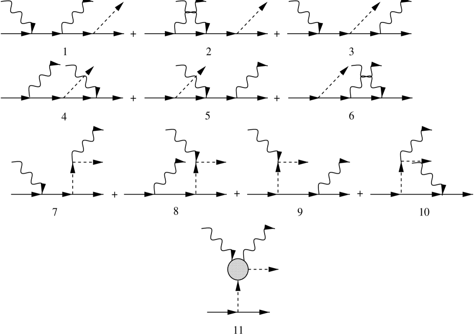
The cross section of the process $\gamma p\to\gamma\pi^{+}n$ has been calculated in the framework of two different models. In the first model (model-1) the contribution of all the pion and nucleon pole diagrams is taken into account using pseudoscalar pion-nucleon coupling (fig. 2) [35].

In the second model (model-2), we include the nucleon and the pion pole diagrams without the anomalous magnetic moments of the nucleons (fig. 3a-e), and in addition the contributions of the resonances $\Delta(1232)$, $P_{11}(1440)$, $D_{13}(1520)$, and $S_{11}(1535)$ according to fig. 3f. The amplitude of the $\gamma\pi^{+}$ elastic scattering in this model is described by eq. (6). We will determine the pion polarizability by comparing the experimental data with predictions of these theoretical models in different regions of $s_{1}$. Therefore, we limited ourselves to describing the baryon resonances by the diagram fig. 3f only, because this diagram has a pole at $s_{1}=m_{\pi}^{2}$. The details of the calculations of these resonance contributions are given in the Appendices.

It should be noted that the contribution of the sum of the pion polarizabilities is very small in the considered region of $140^{\circ}\lesssim\theta^{cm}_{\gamma\gamma`}\lesssim 180^{\circ}$ . The estimate shows that the contribution of $(\alpha+\beta)_{\pi^{\pm}}=0.4$ to the value of $(\alpha-\beta)_{\pi^{\pm}}$ is less than 1%.

3 Experimental setup

The experiment has been performed at the continuous-wave electron accelerator MAMI B [36, 37] using Glasgow-Mainz photon tagging facility [38, 39]. The quasi-monochromatic photon beam covered an energy range from 537 to 819 MeV with an intensity $\sim 0.6\times 10^{6}\gamma/$s in the tagger channel with a 2.3 MeV wide bite for the lowest photon energy. The average energy resolution was 2 MeV. The tagged photons entered a scattering chamber, containing a 3 cm diameter and 11.4 cm long liquid hydrogen target with Kapton windows. The target was aligned along the photon beam direction. The emitted photon $\gamma^{\prime}$, the $\pi^{+}$-meson, and the neutron were detected in coincidence. The experimental setup is shown in fig. 4.

The photons were detected by the spectrometer TAPS [40, 41], assembled in a special configuration (fig. 5). The TAPS spectrometer consists of 528 BaF₂ crystals, each 250 mm long (corresponding to 12 radiation lengths) and hexagonally shaped with an inner diameter of 59 mm. All crystals were arranged into three blocks. Two blocks (A,B) consisted of 192 crystals arranged in 11 columns and the third block (C) had 144 crystals arranged in 11 columns. These three blocks were located in the horizontal plane around the target at central angles $68^{\circ}$, $124^{\circ}$, $180^{\circ}$ with respect to the beam axis. Their distances to the target center were 55 cm, 50 cm and 55 cm, respectively. All BaF₂ modules were equipped with 5 mm thick plastic veto detectors for the identification of charged particles.

The neutrons were detected by a wide aperture time-of-flight spectrometer (TOF) [42]. It consisted of 111 scintillation-detector bars of dimensions $50\times 200\times 3000$ mm³ and 16 counters ($10\times 230\times 3000$ mm³) which were used as charged-particles veto detectors. The bars are made from NE110 plastic scintillator and each bar is read out at each end by a $3^{\prime\prime}$ phototube type XP2312B. All bars were assembled in planes 8 deep, each plane having 16 detectors (fig. 4). This block of plastic scintillators and detected neutrons in the energy region 10-100 MeV with efficiencies varying between $30$ to $50\%$ depending on energy. The neutron energy determination was by time of flight and for the present energy range and path the FWHM resolution was $\sim 10\%$. Accuracy of the horizontal position of TOF was $\pm 10$ cm and the FWHM resolution of its vertical position was 29 cm [43].

In order to detect the $\pi^{+}$-meson two two-coordinate multi-wire proportional chambers (MWPC) and a forward scintillator detector (FSD) have been developed and constructed (fig. 6), which provided a fast trigger signal. The MWPCs were located at $0^{\circ}$ with respect to the beam direction. Their sensitive areas covered angles in the laboratory system $\theta\cong 2^{\circ}-20^{\circ}$, $\varphi\cong 0^{\circ}-360^{\circ}$. The MWPCs have the following characteristics:

• sensitive region: $292\times 292$ mm²,

• photon-beam aperture: $40\times 40$ mm²,

• anode wires: gold plated tungsten $20~{}\mu$m,

• distance between wires: 2 mm,

• cathode planes: $25~{}\mu$m aluminum foil,

• gas windows: $50~{}\mu$m mylar foil,

• anode-cathode gap: 5 mm,

• maximum current for all wires: $100~{}\mu$A.

Each MWPC has two perpendicular planes each with 128 wires.

The MWPCs operated with a gas mixture of Argon ($60\%$) and Isobutane ($30\%$). The gas mixture was blown through the chambers at a flow rate of 180 ml/min. MWPCs were read by LeCroy 2735 DC cards. The FSD had 16, $1\times 2\times 30$ cm³ plastic scintillator strips with a $4\times 4$ cm² hole in the middle for the photon beam. Each strip was read out by a single photomultiplier tube.

The MWPCs were optimized for high count rates and good efficiency, described as follows. The measurement of the efficiency was carried out with a ⁹⁰Sr beta source. The MWPC was placed between two $190\times 20\times 5$ mm³ plastic scintillators. This detector arrangement was irradiated by a radioactive source, viewed through a two millimeter collimator. Thresholds of the discriminators for the plastic detectors were fixed at 30 mV. Double coincidence rates between the plastic detectors and triple coincidences which included the MWPC were measured simultaneously at different thresholds of the LeCroy 2735 DC cards, for different values of the MWPC high voltage. A high voltage for MWPC of 3.25 kV with 3 V threshold for the LeCroy 2735 DC cards was chosen where the maximum efficiency was about 98 % and the noise was suppressed.

In order to optimize the MWPC and FSD for high counting rates, a test measurement was carried out with untagged bremsstrahlung produced at the tagger radiator ($E_{e}=855$ MeV). The first MWPC was positioned at a distance of 131 cm from the end of the vacuum beam pipe. A mylar target of 3 mm thickness was placed at a distance of 45 cm from the foil covering the first chamber. Thresholds of the FSD discriminators were set to $500\pm 50$ keV on the basis of the Compton electron response to ⁶⁰Co $\gamma$ rays. The test run results are presented in table 2. We found that at the maximum intensity in the tagging system (beam current $\sim 150$ nA) the current of the MWPC was $76~{}\mu$A, well within operational limits.

In the experiment on the radiative pion photoproduction the first MWPC was centered at a polar angle of $0^{\circ}$ with respect to the beam axis, and at a distance of 46 cm from the center of the target to the first wire plane. The second MWPC was placed $\sim 10$ cm behind the first one and was rotated $45^{\circ}$ in azimuth with the respect to the front chamber. The FSD was positioned between the first and second MWPCs. After the commissioning of this experiment in the A2 Tagger Hall at Mainz, triple coincidence of $\gamma$, $\pi^{+}$, and $n$ were taken over a period of 1150 hours.

4 Determination of the $\pi^{+}$-meson polarizability

4.1 Analysis of the experimental data

In order to determine an efficiency of the $\gamma$ and $\pi^{+}$ detectors and to check the normalization of the experimental data, $\pi^{0}$-meson photoproduction from the proton has been measured and the obtained cross section was compared with the well-known values [44].

Neutral pions produced in the liquid hydrogen target were detected via their two-photon decay with the TAPS spectrometer. The MWPC and FSD were used to detect the protons, triggered by a coincidence between TAPS and FSD. About $2.5\times 10^{6}$ raw events were collected and after kinematic selection $\sim 5\times 10^{5}$ events remained. The background of multiple pion production was removed by reconstructing the missing mass spectrum for the reaction $\gamma p\to\pi^{0}X$. Random coincidences were subtracted by samples selected outside the prompt coincidence time window with the photon tagger.

The cross section was obtained using the detector yields, the detection efficiency of each detector arm, the thickness of the liquid hydrogen target, and the intensity of the photon beam. The photon intensity was determined by counting the electrons detected in the tagging spectrometer focal plane detector. The tagging efficiency, i.e. the probability of a bremsstrahlung photon passing through the collimator giving an $e^{-}$ hit in the focal plane, was determined by comparing the number of electrons detected in the tagger to the number of photons detected in a 100% efficient lead glass detector, which was moved into the photon beam during special runs at very low beam intensity. The angle and energy dependent detection efficiency of TAPS and FSD+MWPC was calculated by Monte Carlo using GEANT3 [45], in which all relevant properties of the setup are taken into account. As result we obtained experimental data for the process $\gamma p\to\pi^{0}p$ for the angles $140^{\circ}$, $150^{\circ}$, $160^{\circ}$, and $170^{\circ}$ in the energy region $290-810$ MeV.

The angular distribution data in the energy region $480-530$ MeV are shown in fig. 7. The filled circles are the data of the present work. The open circles are the data obtained in [44]. The results of the theoretical models MAID and DMT are depicted by the solid and dashed curves, respectively. The dotted lines are the results of the partial wave analysis SAID of the world data.

The present angular distributions are in a good agreement with those of ref. [44] and with the predictions of MAID, DMT and SAID for incoming photon energy up to $\sim 650$ MeV. This result shows that the efficiencies of the $\gamma$ and $\pi^{+}$-meson detectors correspond well to the simulation result.

To determine the efficiency of the TOF detector, GEANT was improved by the STANTON program package [46], which allowed one to consider more correctly an interaction of the low energy neutrons with the plastic scintillator and to convert the ionization losses of different charged particles into the electron equivalent. The accuracy of this simulation is limited by the uncertainty of the cross sections of the elastic scattering of the neutrons with the protons in the scintillators of 2%. This has to be added to the inaccuracy of GEANT for the efficiency calculation of the whole setup. In ref. [44] a similar setup has been investigated with GEANT and the results have been compared to the accurately measured $p(\gamma,\pi^{0})p$ reaction giving an uncertainty of 3%. Adding these two contributions quadratically results in 4% for the systematic error of the overall efficiency of the experimental setup.

In order to check the functioning of the neutron detector, data on double pion photoproduction $\gamma p\to\pi^{0}\pi^{+}n$ were selected and analyzed. To this aim, the $\pi^{0}$-meson was reconstructed via the invariant mass of the two decay photons and then, using the reconstructed momentum of the neutron, the missing mass spectrum for the $\pi^{+}$-meson was constructed. Alternatively, the invariant mass of the $\pi^{0}$ and neutron gave a prominent peak, the width and the position of which corresponded to the $\Delta^{0}(1232)$ resonance. The analysis of the data obtained for the process $\gamma p\to\pi^{0}\pi^{+}n$ indicated that it proceeds mainly through excitation of the $\Delta^{0}(1232)$ resonance in our kinematical region in agreement with the finding of ref. [47]. The investigation of this process showed that the selection of the neutrons and determination of their parameters was correct.

The process $\gamma p\to\gamma\pi^{+}n$ was detected by counting the triple coincidences of the emitted photon, the $\pi^{+}$-meson, and the neutron. Coincident pulses from TAPS and FSD were used as a pre-trigger. This signal was a ”stop” for the tagger focal plane and a ”start” for TAPS and TOF Time Digital Convertors (TDC). Slightly later coincidence information from the tagger and TOF then determined if the event was stored or cleared.

The main source of spurious correlated contributions to $\gamma p\to\gamma\pi^{+}n$ comes from the $\gamma p\to\pi^{0}\pi^{+}n$ reaction. This background was simulated using the total cross section measured at MAMI [48] and was suppressed by using conservation of energy and momentum. To this end we compared in the analysis the invariant variables $t$, $s_{1}$ and $t_{1}$ with the variables $t^{\prime}$, $s_{1}^{\prime}$, and $t_{1}^{\prime}$ determined from the measured data by two different methods [49]. The values of $t$ were determined according to eq. (2.2) when the neutron energy was measured by the TOF detector. In the case of $t^{\prime}$ this energy was calculated from the equations of the energy and momentum conservation and $t^{\prime}=f_{1}(E_{\gamma},E_{\gamma^{\prime}},\theta_{\gamma\gamma^{\prime}},\theta_{\gamma\pi^{+}},\theta_{\gamma^{\prime}\pi^{+}})$. The variable $t_{1}$ was evaluated as function of $E_{\gamma}$, $E_{\gamma^{\prime}}$, and $\theta_{\gamma\gamma^{\prime}}$. For $t_{1}^{\prime}$ the energy and the angle of the final photon were expressed through other measured variables and $t_{1}^{\prime}=f_{2}(E_{\gamma},E_{n},\theta_{\gamma n},\theta_{\gamma\pi^{+}},\theta_{\pi^{+}n})$. In the case of $s_{1}$ and $s_{1}^{\prime}$ we had $s_{1}=f_{3}(E_{\gamma},E_{n},\theta_{\gamma n})$ and $s_{1}^{\prime}=f_{4}(E_{\gamma},E_{\gamma^{\prime}},\theta_{\gamma\gamma^{\prime}},\theta_{\gamma\pi^{+}},\theta_{\gamma^{\prime}\pi^{+}})$.

The constraint that $(t-t^{\prime})<0.5m_{\pi}^{2}$, $(s_{1}-s_{1}^{\prime})<0.5m_{\pi}^{2}$, $(t_{1}-t_{1}^{\prime})<0.7m_{\pi}^{2}$ was applied. Such a kinematic cut, which was chosen on the basis of the simulation, suppressed the background to the $3\%$ level relative to the $\gamma p\to\gamma\pi^{+}n$ process.

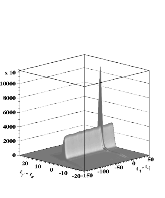
Prompt and random coincidence regions were determined from a two dimensional triple-coincidence spectrum (fig. 8) where the time difference between the initial $\gamma$ and the final $\gamma^{\prime}$ photons $(t_{\gamma}-t_{\gamma^{\prime}})$, detected by the tagger and TAPS, and the difference between the final $\gamma^{\prime}$ photon and the $\pi^{+}$-meson $(t_{\gamma^{\prime}}-t_{\pi^{+}})$, detected by TAPS and FSD, are displayed at the horizontal axes. The sharp peak in this figure corresponds to the triple coincidence of the reaction under study. The ridge along the $(t_{\gamma}-t_{\gamma^{\prime}})$ axis and the plateau are the contributions of random double coincidences for the initial $\gamma$ and final $\gamma^{\prime}$ photons and for TAPS–FSD, respectively. The yield was calculated by subtracting the numbers of the random coincidences for two photons and TAPS–FSD with appropriate weights given by the relative width of the cuts, from the number of the events under the sharp peak.

A missing-mass spectrum of the reaction $\gamma p\to\gamma nX$, constructed using the photon and the neutron momenta measured in this experiment, is shown in fig. 9. This spectrum shows a peak at $M_{X}=139.7$ MeV with a resolution $\sigma=20$ MeV corresponding to the $\pi^{+}$-meson. It agrees well with the simulation results. As seen from this figure, a clean separation of radiative $\pi^{+}$-meson photoproduction on the proton from the competing background reaction $\gamma p\to\pi^{0}\pi^{+}n$ is obtained.

As result we have identified about $4\times 10^{5}$ radiative $\pi^{+}$-meson photoproduction events in the kinematic region: $E_{\gamma}=537-817MeV$, $1.5m_{\pi}^{2}\leq s_{1}\leq 15m_{\pi}^{2}$, $-12m_{\pi}^{2}<t<t_{max}$, $140^{\circ}\leq\theta_{\gamma\gamma^{\prime}}^{cm}<180^{\circ}$.

4.2 Derivation of the polarizability

In order to reduce the influence of the nucleon resonances, the differential cross section was integrated over the angles $\theta_{\gamma\gamma^{\prime}}^{cm}$ from $140^{\circ}$ to $180^{\circ}$ and $\varphi_{b}$ from $0^{\circ}$ to $360^{\circ}$.

To increase our confidence that the model dependence of the result is under control we limited ourselves to kinematic regions where the difference between model-1 and model-2 did not exceed $3\%$ when $(\alpha-\beta)_{\pi^{+}}$ is constrained to zero. First, we consider the kinematic region where the contribution of the pion polarizability is negligible, i.e. the region $1.5m_{\pi}^{2}\leq s_{1}<5m_{\pi}^{2}$.

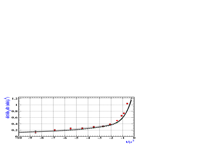
In fig. 10, the experimental data for the differential cross section, averaged over the full photon beam energy interval from 537 MeV up to 817 MeV and over $s_{1}$ in the indicated interval, are compared to predictions of model-1 (dashed curve) and model-2 (solid curve). The dotted curve is the fit of the experimental data in the region of $-10m_{\pi}^{2}<t<-2m_{\pi}^{2}$. As seen from this figure, the theoretical curves are very close to the experimental data. This means that the dependence of the differential cross section on the square of the four momentum transfer $t$ which is basically the kinetic energy of the neutron (see eq. (2.2)) is well reproduced by using the mentioned GEANT simulations for the efficiency. On the other side, there is a small difference of less than 10% in the absolute overall efficiency which could be due to a theoretical, an experimental, or both deviation from the true cross section. However, since we are only interested in the change of the curves with $(\alpha-\beta)_{\pi^{\pm}}$ we slightly adjusted the experimental cross section to the theoretical.

Then we investigated the kinematic region where the polarizability contribution is biggest. This is the region $5m_{\pi}^{2}\leq s_{1}<15m_{\pi}^{2}$ and $-12m_{\pi}^{2}<t<-2m_{\pi}^{2}$. In the range $t>-2m_{\pi}^{2}$ the polarizability contribution is small and also the efficiency of the TOF is not well known here. Therefore, we have excluded this region.

In the considered region of the phase space, with maximum sensitivity of the cross section to the polarizability but small differences between the considered theoretical models, we obtained the cross section of the process $\gamma p\to\gamma\pi^{+}n$ integrated over $s_{1}$ and $t$. All events are divided into 12 bins of the initial photon energy. For each bin $i$, the cross section $\sigma^{i}$ is calculated from

$$\sigma^{i}=Y^{i}/\varepsilon^{i}N^{i}_{\gamma}N_{t},$$ (14)

where $Y^{i}$ is the number of the selected events after background subtractions, $\varepsilon^{i}$ the detection efficiency for the $\gamma p\to\gamma\pi^{+}n$ channel, $N_{t}$ the number of protons per area in the 11.4 cm of the $LH_{2}$ target, and $N^{i}_{\gamma}$ the number of photons passing through the target in the same time interval as for the integration of $Y^{i}$.

The cross sections are calculated according to model-1 and model-2 for two different values of $(\alpha-\beta)$ within the phase space covered by the experiment. The obtained experimental cross sections and their theoretical predictions for $(\alpha-\beta)_{\pi^{+}}=0$ and $14\times 10^{-4}{\rm fm}^{3}$ are presented in fig. 11. The error bars are the quadratic sum of statistical and systematic errors.

The systematic error is due to the uncertainties of the time and kinematic cuts ($\pm 1\%$ for each cut), the number of target protons ($\pm 1.5\%$), the photon flux ($\pm 2\%$), and the detection efficiency calculations ($\pm 4\%$). As a result, we get the limiting systematic deviation for the cross section of $\pm 5\%$. This is equivalent to a rectangular error distribution with a $\pm 5\%$ limit. The root-mean square error of this distribution is then $\sigma_{syst}=5/\sqrt{3}\%\simeq 3\%$.

Comparing these experimental data with predictions of the models we find values of $(\alpha-\beta)^{i}_{\pi^{+}}$ and corresponding errors $\Delta_{stat}(\alpha-\beta)^{i}_{\pi^{+}}$ and $\Delta_{syst}(\alpha-\beta)^{i}_{\pi^{+}}$ for each experimental point $i$.

As an example of such a procedure, fig. 12 shows the experimental value of the cross section at $E_{\gamma}=653$ MeV with statistical and systematic errors and the dependence of the cross section on $(\alpha-\beta)_{\pi^{+}}$ calculated in the framework of model-1. Comparing these experimental data with the model predictions we obtain for this energy bin

$$(\alpha-\beta)_{\pi^{+}}=9.03^{+3.58(stat)+3.12(syst)}_{-3.28(stat)-2.89(syst)}.$$ (15)

This result has slightly asymmetric errors, but making the approximation that they are symmetrical and taking their average values, the value of $(\alpha-\beta)_{\pi^{+}}$ is obtained by averaging over all 12 bins of $E_{\gamma}$ as

$$(\alpha-\beta)_{\pi^{+}}=\frac{\sum_{i}(\alpha-\beta)^{i}_{\pi^{+}}w_{i}}{\sum_{i}w_{i}},$$ (16)

where $w_{i}=1/(\Delta_{stat}(\alpha-\beta)^{i}_{\pi^{+}})^{2}$.

The statistical error for the averaged value $(\alpha-\beta)_{\pi^{+}}$ is calculated as

$$\Delta_{stat}(\alpha-\beta)_{\pi^{+}}=(\sum_{i}w_{i})^{-1/2}.$$ (17)

The systematic errors are correlated for the cross sections at the different values of the energy $E_{\gamma}$. They give contributions to the systematic errors for $(\alpha-\beta)^{i}_{\pi^{+}}$ at different $i$ having different statistical weights. Therefore, the systematic error $\Delta_{syst}(\alpha-\beta)_{\pi^{+}}$ is determined by calculating a weighted average as follows:

$$\Delta_{syst}(\alpha-\beta)_{\pi^{+}}=\frac{\sum_{i}\Delta_{syst}(\alpha-\beta)^{i}_{\pi^{+}}w_{i}}{\sum_{i}w_{i}}.$$ (18)

Using this procedure separately for each model, we obtain:

$$(\alpha-\beta)_{\pi^{+}}=(12.2\pm 1.6_{stat}\pm 3.3_{syst})\times 10^{-4}{\rm fm}^{3}\qquad{\rm(model-1)},$$ (19)

$$(\alpha-\beta)_{\pi^{+}}=(11.1\pm 1.4_{stat}\pm 2.8_{syst})\times 10^{-4}{\rm fm}^{3}\qquad{\rm(model-2)}.$$ (20)

As indicated above, the dominant systematic error is caused by the uncertainties in the neutron detector efficiency. However, this is a difficult problem to overcome because better neutron detectors are hardly possible.

An additional independent analysis [50] of the experimental data was carried out by a constrained $\chi^{2}$ fit [51]. The reaction $\gamma p\to\gamma\pi^{+}n$ is identified by 15 quantities for the momenta of all five participating particles. In this experiment 14 quantities were measured for each event, the complete 4-momenta of all particle except the pion for which only the direction angles were measured. Considering the over-determined situation, a constrained $\chi^{2}$ fit was employed to determine how well the measured event detection angles $(\theta,\,\varphi)$ agreed with the measured momenta magnitudes $P$, and as well to give the optimum $(\theta,\,\varphi,\,P)$ values for each event for all five participating particles. To assure convergence, the variations were done only for the magnitudes of the final state momenta. All combinations of measured particles were tested to see which best satisfy the $\gamma p\to\gamma\pi^{+}n$ reaction. This method allows us for each event to find the combination of measured particles which best fit the $\gamma p\to\gamma\pi^{+}n$ reaction kinematics. The $P$ values best fitting $(\theta,\,\varphi)$ correspond to the minimum of the constructed constrained $\chi^{2}$ functional.

Simulation studies of the constrained fit method showed that the described reconstruction algorithm based on the kinematic fit $\chi^{2}$ selection criteria can be successfully used for the suppression of the double pion photoproduction background and reconstruction of the $\gamma p\to\gamma\pi^{+}n$ reaction.

A series of seven analyses with $\chi^{2}<4,\,5,\,6,\,7,\,8,\,9,\,10$ has been performed. The value for $(\alpha-\beta)_{\pi^{+}}$ stabilizes for $\chi^{2}<5$ and the values for $\chi^{2}<4$:

$$(\alpha-\beta)_{\pi^{+}}=(10.1\pm 2.6_{stat}\pm 3.0_{syst})\times 10^{-4}{\rm fm}^{3}\qquad{\rm(model-1)},$$ (21)

$$(\alpha-\beta)_{\pi^{+}}=(10.3\pm 2.3_{stat}\pm 2.7_{syst})\times 10^{-4}{\rm fm}^{3}\qquad{\rm(model-2)}$$ (22)

agree very well with the first analysis giving it additional support. However the statistical accuracy of this method is less significant and, therefore, we give the result of the optimized cut analysis (19), (20), averaged for model-1 and model-2:

$$(\alpha-\beta)_{\pi^{+}}=(11.6\pm 1.5_{stat}\pm 3.0_{syst}\pm 0.5_{model})\times 10^{-4}{\rm fm}^{3}.$$ (23)

5 Discussion

The experimental result (23) for the difference $(\alpha-\beta)_{\pi^{+}}$ of the electric and magnetic polarizabilities provides an important piece of information about the hadronic structure of the pion as tested with soft external electromagnetic fields. Moreover, from a theoretical point of view, there is another reason for the extraordinary interest in and importance of a precise experimental determination of the charged-pion polarizabilities. The approximate $\mbox{SU}(2)_{L}\times\mbox{SU(2)}_{R}\times\mbox{U}(1)_{V}$ chiral symmetry in the two-flavor sector of QCD results in a Ward identity which relates Compton scattering on a charged pion, $\gamma\pi^{+}\to\gamma\pi^{+}$, to radiative charged-pion beta decay, $\pi^{+}\to e^{+}\nu_{e}\gamma$. The corresponding low-energy theorem was originally derived by Terentev [52] in the framework of the partially conserved axial-vector current (PCAC) hypothesis in combination with current algebra. This PCAC prediction is equivalent to the result obtained using chiral perturbation theory at leading non-trivial order (${\cal O}(p^{4})$) and can be written in the form

$$\alpha_{\pi^{+}}=-\beta_{\pi^{+}}=2\frac{e^{2}}{4\pi}\frac{1}{(4\pi F_{\pi})^{2}\mu}\frac{\bar{l}_{6}-\bar{l}_{5}}{6},$$ (24)

where $F_{\pi}=92.4$ MeV is the pion decay constant and $(\bar{l}_{6}-\bar{l}_{5})$ is a linear combination of scale-independent parameters of the Gasser and Leutwyler Lagrangian [53]. At lowest non-trivial order $({\cal O}(p^{4}))$ this difference is related to the ratio $\gamma=F_{A}/F_{V}$ of the pion axial-vector form factor $F_{A}$ and the vector form factor $F_{V}$ of radiative pion beta decay [53]:

$$\gamma=\frac{1}{6}(\bar{l}_{6}-\bar{l}_{5}).$$

Once this ratio is known, chiral symmetry makes an absolute prediction for the polarizabilities. This situation is similar to the case of $\pi\pi$ scattering [54], where the $s$-wave $\pi\pi$-scattering lengths are predicted once $F_{\pi}$ has been determined from pion decay. Using the most recent determination $\gamma=0.443\pm 0.015$ by the PIBETA Collaboration [55] (assuming $F_{V}=0.0259$ obtained from the conserved vector current hypothesis) results in the ${\cal O}(p^{4})$ prediction

$$\alpha_{\pi^{+}}=(2.64\pm 0.09)\times 10^{-4}\,\mbox{fm}^{3},$$

where the estimate of the error is only the one due to the error of $\gamma$ and does not include effects from higher orders in the quark mass expansion. Clearly, there will be corrections to the prediction of eq. (24). The results of a two-loop analysis (${\cal O}(p^{6})$) of the charged-pion polarizabilities have been worked out in ref. [3]:

$$(\alpha+\beta)_{\pi^{+}} = (0.3\pm 0.1)\times 10^{-4}\,\mbox{fm}^{3},$$ (25)

$$(\alpha-\beta)_{\pi^{+}} = (4.4\pm 1.0)\times 10^{-4}\,\mbox{fm}^{3}.$$ (26)

First of all, we note that the degeneracy $\alpha=-\beta$ has been removed at ${\cal O}(p^{6})$. The corresponding corrections amount to an 11% (22%) change of the ${\cal O}(p^{4})$ result for $\alpha_{\pi^{+}}$ ($\beta_{\pi^{+}}$), indicating a similar rate of convergence as for the $\pi\pi$-scattering lengths [53, 56]. The effect of the new low-energy constants appearing at ${\cal O}(p^{6})$ on the pion polarizability was estimated via resonance saturation by including vector- and axial-vector mesons. The contribution was found to be about 50% of the two-loop result. However, one has to keep in mind that ref. [3] could not yet make use of the improved analysis of radiative pion decay which, in the meantime, has also been evaluated at two-loop accuracy [57, 58]. Taking higher orders in the quark mass expansion into account, Bijnens and Talavera obtain $(\bar{l}_{6}-\bar{l}_{5})=2.98\pm 0.33$ [57], which would slightly modify the leading-order prediction to $\alpha_{\pi^{+}}=(2.96\pm 0.33)\times 10^{-4}\,\mbox{fm}^{3}$ instead of $\alpha_{\pi^{+}}=(2.7\pm 0.4)\times 10^{-4}\,\mbox{fm}^{3}$ used in ref. [3]. Accordingly, the difference $(\alpha-\beta)_{\pi^{+}}$ of eq. (26) would increase to $4.9\times 10^{-4}\,\mbox{fm}^{3}$ instead of $4.4\times 10^{-4}\,\mbox{fm}^{3}$, whereas the sum would remain the same as in eq. (25). A value of $4.9\times 10^{-4}\,\mbox{fm}^{3}$ deviates by 2 standard deviations from the experimental result of eq. (23). Nevertheless, both the precision measurement of radiative pion beta decay [55] and of radiative pion photoproduction indicate that further theoretical and experimental work is needed. In particular, the analysis of ref. [55] suggests an inadequacy of the present $V-A$ description of the radiative beta decay, which would also reflect itself in an inadequacy of the ChPT description in its present form.

A different approach for obtaining a theoretical prediction for the difference $(\alpha-\beta)$ is the application of dispersion sum rules (DSR). In ref. [5] dispersion relations at a fixed value of the Mandelstam variable $u=\mu^{2}$ without subtraction were applied to the helicity amplitude $M_{++}$ of elastic $\gamma\pi$ scattering:

$$(\alpha-\beta)=\frac{1}{2\pi^{2}\mu}\left\{\int\limits_{4\mu^{2}}^{\infty}\frac{ImM_{++}(t^{\prime},u=\mu^{2})\,dt^{\prime}}{t^{\prime}}+\int\limits_{4\mu^{2}}^{\infty}\frac{ImM_{++}(s^{\prime},u=\mu^{2})\,ds^{\prime}}{s^{\prime}-\mu^{2}}\right\}.$$ (27)

The biggest contribution to this DSR is given by the strong $s$-wave $\pi\pi$ interaction in the $t$ channel. This interaction can be effectively described by the $\sigma$ meson using a broad Breit-Wigner resonance expression. The parameters of such a $\sigma$ meson have been determined in ref. [6] from a fit to the experimental data for the $\gamma\gamma\to\pi^{0}\pi^{0}$ process (see eq. (7)). A saturation of the DSR (27) by the $\rho(770)$, $b_{1}(1235)$, $a_{1}(1260)$, and $a_{2}(1320)$ mesons in the $s$ channel and the $\sigma$, and $f_{0}(980)$ mesons in the $t$ channel leads to [6]

$$\quad\rho\qquad a_{1}\qquad b_{1}\quad\;a_{2}\quad\;\;f_{0}\qquad\sigma$$

$$(\alpha-\beta)^{DSR}_{\pi^{+}} = -1.2+2.1+0.9-1.4+0.4+9.5=(10.3\pm 1.9)\times 10^{-4}{\rm fm}^{3},$$ (28)

where the error indicated for this value is caused by the error for the $\sigma$ meson parameters. This value of $(\alpha-\beta)_{\pi^{+}}$ is in agreement with the experimental result of eq. (23) but differs significantly from the ChPT result of eq. (26). On the other hand, the DSR for $(\alpha-\beta)_{\pi^{0}}$ yields [6]

$$\quad\;\rho\qquad\;\;\omega\qquad\;\;\varphi\qquad\;f_{0}\qquad\;\;\;\sigma$$

$$(\alpha-\beta)^{DSR}_{\pi^{0}} = -1.79-11.69-0.04+0.44+10.07=(-3.01\pm 2.06)\times 10^{-4}{\rm fm}^{3}$$ (29)

which, within the errors, is not in conflict with the two-loop ChPT predictions $\alpha_{\pi^{0}}=(-0.35\pm 0.10)\times 10^{-4}\,\mbox{fm}^{3}$ and $\beta_{\pi^{0}}=(1.50\pm 0.20)\times 10^{-4}\,\mbox{fm}^{3}$ [2] and with the experimental values $(\alpha-\beta)_{\pi^{0}}=(-1.6\pm 2.2)\times 10^{-4}{\rm fm}^{3}$ and $(-0.6\pm 1.8)\times 10^{-4}{\rm fm}^{3}$ obtained in refs. [6] and [19], respectively.

One might ask for explanations of the difference between ChPT and our experiment without questioning the validity of ChPT. The most obvious idea is to consider the ”off-shellness” of the initial pion. Clearly, this issue cannot be addressed consistently as an independent effect [59, 60] and would require a more sophisticated analysis such as, e.g., a full ChPT calculation at the one-loop level which is beyond the scope of the present work. However, in order to obtain an estimate of this effect, we have calculated $(\alpha-\beta)_{\pi^{+}}$ with the help of dispersion relations for a mass of the initial pion equal to $t$ and found that such a correction is less than 5%.

6 Conclusion

A measurement of radiative $\pi^{+}$ photoproduction from the proton ($\gamma p\to\gamma\pi^{+}n$) was carried out at the Mainz tagged photon facility in the kinematic region 537 MeV $<E_{\gamma}<~{}817$ MeV, $140^{\circ}~{}\leq\theta_{\gamma\gamma^{\prime}}^{cm}\leq~{}180^{\circ}$. The difference of the electric and magnetic $\pi^{+}$-meson polarizabilities has been determined from a comparison of the experimental data with predictions of two different theoretical models which included or neglected baryon resonances. In order to reduce the contribution of the baryon resonances, the differential cross section was integrated over $\theta_{\gamma\gamma^{\prime}}^{cm}$ from $140^{\circ}$ to $180^{\circ}$ and over $\varphi$ from $0^{\circ}$ to $360^{\circ}$. To further reduce the model dependence, the kinematic region was chosen such that the difference between the predictions of the two considered models did not exceed $3\%$ for $(\alpha-\beta)_{\pi^{+}}=0$.

The experimental detection efficiency was normalized by comparing the theoretical predictions with the experimental differential cross sections in the kinematic region where the pion polarizability contribution is negligible $(1.5<s_{1}/m_{\pi}^{2}<5)$.

In the region, where the pion polarizability contribution is substantial ($5<s_{1}/m_{\pi}^{2}<15$, $-12<t/m_{\pi}^{2}<-2$), the difference of the electric and magnetic $\pi^{+}$-meson polarizabilities was determined by the comparison of the experimental data for the cross section of radiative pion photoproduction with the predictions of two theoretical models under consideration. As a result we have obtained: $(\alpha-\beta)_{\pi^{+}}=(11.6\pm 1.5_{stat}\pm 3.0_{syst}\pm 0.5_{model})\times 10^{-4}{\rm fm}^{3}$. This result is consisted with the result of ref. [10] and at variance with recent calculations in the framework of chiral perturbation theory.

Appendix A

The contribution of the diagram in fig. 3 for the $\Delta(1232)$ resonance to the amplitude of the process under consideration can be written as

$$T_{\Delta} = \frac{-2e^{2}(\varepsilon_{2}q_{2})g_{0}(s)/m_{\pi}}{(s_{1}-m_{\pi}^{2})(s-M^{2}_{\Delta}+iM_{\Delta}\Gamma(s))}\bar{u}(p_{2})q^{\mu}\Delta_{\mu\nu}(p)\gamma_{5}$$

$$\times\left[-(g_{1}(s)/m)(k_{1}^{\nu}\hat{\varepsilon}_{1}-\varepsilon_{1}^{\nu}\hat{k}_{1})+(g_{2}(s)/m^{2})(k_{1}^{\nu}(p_{1}\varepsilon_{1})-\varepsilon_{1}^{\nu}(p_{1}k_{1}))\right]u(p_{1}),$$

where

$$\Delta_{\mu\nu}(p)=(1/3M^{2}_{\Delta})(\hat{p}+M_{\Delta})(2p_{\mu}p_{\nu}-3M^{2}_{\Delta}g_{\mu\nu}+M^{2}_{\Delta}\gamma_{\mu}\gamma_{\nu}+M_{\Delta}(\gamma_{\mu}p_{\nu}-\gamma_{\nu}p_{\mu})),$$ (A2)

$p=p_{1}+k_{1}$, $q=q_{2}+k_{2}$ and $\Gamma$ is the decay width of the $\Delta(1232)$ resonance.

In accordance with refs. [61, 62] the following parametrization is used:

$$\Gamma(s)=\Gamma_{0}\left(\frac{|q|}{|q_{\Delta}|}\right)^{3}\frac{M_{d}}{\sqrt{s}}\frac{1+R^{2}|q_{\Delta}|^{2}}{1+R^{2}|q|^{2}},$$

$$g_{0}(s)=g_{0}((1+R^{2}|q_{\Delta}|^{2})/(1+R^{2}|q|^{2}))^{1/2},\qquad|q_{\Delta}|=|q(s=M^{2}_{\Delta})|,$$

$$g_{1,2}(s)=g_{1,2}((1+R^{2}|k_{\Delta}|^{2})/(1+R^{2}|k|^{2}))^{1/2},\qquad|k_{\Delta}|=|k(s=M^{2}_{\Delta})|,$$

$M_{\Delta}=1232$ MeV,  $\Gamma_{0}=109$ MeV,  $R=5.5$ GeV^-1.

According to ref. [62] the coupling constants are taken to be $g_{0}g_{1}/m_{\pi}m=19.78$ GeV^-2 and $g_{0}g_{2}/m_{\pi}m^{2}=-21.2$ GeV^-3.

Since the term at the coupling $g_{2}$ in eq. (Appendix A) gives a major contribution to the $E_{1+}$ electric quadrupole [61], we represent the contribution of the $D_{13}$ resonance as

$$T_{D_{13}} = \frac{-2e^{2}(\varepsilon_{2}q_{2})\bar{g}_{0}(s)/m_{\pi}}{(s_{1}-m_{\pi}^{2})(s-M^{2}_{D}+iM_{D}\bar{\Gamma}(s))}\bar{u}(p_{2})q^{\mu}\gamma_{5}\bar{\Delta}_{\mu\nu}(p)$$ (A3)

$$\times(\bar{g}_{2}(s)/m^{2})[k_{1}^{\nu}(p_{1}\varepsilon_{1})-\varepsilon_{1}^{\nu}(p_{1}k_{1})]u(p_{1}).$$

The propagator $\bar{\Delta}_{\mu\nu}(p)$ is obtained from $\Delta_{\mu\nu}(p)$ by replacing the mass $M_{\Delta}$ by $M_{D}$. We use the same parametrization as for the $\Delta(1232)$ resonance but with the following values of the mass, width, and coupling constants: $M_{D}=1520$ MeV, $\bar{g}_{0}\bar{g}_{2}=0.5g_{0}g_{2}$, $\bar{\Gamma}_{0}=\Gamma_{0}=109$ MeV.

The contribution of the $P_{11}(1440)$ resonance can be written as [62]

$$T_{P_{11}} = \frac{-2e^{2}(\varepsilon_{2}q_{2})g_{0}^{*}}{(s_{1}-m_{\pi}^{2})(s-M^{2}_{P}+iM_{P}\Gamma_{P}(s))}\bar{u}(p_{2})\gamma_{5}(\hat{p}_{1}+\hat{k}_{1}+M_{P})$$ (A4)

$$\left[(g_{1}^{*}/2M_{P})\hat{k}_{1}\hat{\varepsilon}_{1}+(g_{2}^{*}/M^{2}_{P})\left((p_{1}\varepsilon_{1})\hat{k}_{1}-(p_{1}k_{1})\hat{\varepsilon}_{1}\right)\right]u(p_{1}),$$

where $M_{P}$ is the mass of the $P_{11}(1440)$ resonance,

$$\Gamma_{P}(s)=\Gamma_{P0}\frac{(s-m^{2})M_{P}}{(M^{2}_{P}-m^{2})\sqrt{s}},$$

and with the following values of mass, width, and coupling constants [62]: $M_{P}=1440$ MeV, $\Gamma_{P0}=200$ MeV, $g^{*}_{0}g^{*}_{1}/2M_{P}=-2.7$ GeV^-1, and $g^{*}_{0}g^{*}_{2}/M_{P}^{2}=-21.3$ GeV^-2.

The amplitude of the $S_{11}(1535)$ resonance is taken as

$$T_{S_{11}}=\frac{-g_{1S}g_{2S}(\varepsilon_{2}q_{2})}{(s_{1}-m_{\pi}^{2})(s-M^{2}_{S}+iM_{S}\Gamma_{S}(s))}\bar{u}(p_{2})\left[\hat{p}_{2}+\hat{q}+M_{S}\right]\gamma_{5}\hat{\varepsilon}_{1}u(p_{1}),$$ (A5)

where $M_{S}$ is the mass of the $S_{11}(1535)$ resonance and

$$g^{2}_{1S}=\frac{8\pi\Gamma_{S\to\gamma p}M_{S}^{3}}{(M^{2}_{S}-m^{2})(M^{2}_{S}+m^{2}+4mM_{S})},$$

$$g^{2}_{2S}=\frac{8\pi\Gamma_{S\to\pi n}M^{2}_{S}}{q(M_{S})[(M_{S}+m)^{2}-m_{\pi}^{2}]},$$

with $M_{S}$=1535 MeV, $\Gamma_{S}$=150 MeV, $\Gamma_{S\to\gamma p}$=375 MeV, and $\Gamma_{S\to\pi n}$=75 MeV.

However, the considered amplitudes of the nucleon resonances are not gauge invariant and besides the calculations with them are cumbersome. These problems are solved by using the method of orthogonal amplitudes [63, 64, 65].

Appendix B

Let us choose the following basis of orthogonal vectors

$$K = k_{1}+k_{2},$$

$$Q = k_{1}-k_{2},$$

$$P^{\prime} = P-\frac{(PK)}{K^{2}}K-\frac{(PQ)}{Q^{2}}Q,$$ (B1)

$$N_{\mu} = \varepsilon_{\mu\nu\lambda\sigma}P^{\prime\nu}K^{\lambda}Q^{\sigma},$$

where $P=p_{1}+p_{2}$ and $\varepsilon_{0123}=+1$

Let us write the amplitude of the process as

$$\bar{u}(p_{2})Tu(p_{1})=\bar{u}(p_{2})\varepsilon_{2}^{\mu}T_{\mu\nu}\varepsilon_{1}^{\nu}u(p_{1})$$ (B2)

and expand $T_{\mu\nu}$ in terms of the basis vectors $\eta_{\mu}^{\sigma}$

$$T_{\mu\nu}=\sum_{\sigma\sigma\prime}\eta^{\sigma}_{\mu}C_{\sigma\sigma\prime}\eta^{\sigma\prime}_{\nu}.$$ (B3)

Eight products can be constructed from the vectors $\varepsilon_{2}$, $\varepsilon_{1}$, $K$, $Q$, $P^{\prime}$, and $N$:

$$(\varepsilon_{2}K),\quad(\varepsilon_{1}K),\quad(\varepsilon_{2}Q),\quad(\varepsilon_{1}Q),\quad(\varepsilon_{2}P^{\prime}),\quad(\varepsilon_{1}P^{\prime}),\quad(\varepsilon_{2}N),\quad(\varepsilon_{1}N).$$

To reduce the number of possible combinations, we use the gauge invariance conditions:

$$(\varepsilon_{2}k_{2})=(\varepsilon_{1}k_{1})=0,$$ (B4)

$$T_{\mu\nu}k_{1}^{\nu}=k_{2}^{\mu}T_{\mu\nu}=0.$$ (B5)

Then it is evident from (B5) that

$$T_{\mu\nu}(K-Q)^{\nu}=0\quad{\rm or}\quad T_{\mu\nu}K^{\nu}=T_{\mu\nu}Q^{\nu}.$$

If $\eta_{\nu}=K_{\nu}$, then

$$K^{2}=(KQ)=0,$$

and similarly, if $\eta_{\nu}=Q_{\nu}$, then

$$(QK)=Q^{2}=0.$$

However, $K^{2}$ and $Q^{2}$ do not vanish identically. Therefore, the products $(\varepsilon_{i}K)$ and $(\varepsilon_{i}Q)$ are forbidden and as a consequence, only the following combinations remain:

$$(\varepsilon_{2}P^{\prime})(\varepsilon_{1}P^{\prime}),\quad(\varepsilon_{2}N)(\varepsilon_{1}N),$$

$$(\varepsilon_{2}P^{\prime})(\varepsilon_{1}N)\pm(\varepsilon_{2}N)(\varepsilon_{1}P^{\prime}).$$ (B6)

It follows from parity conservation that the coefficients of the first two terms are scalars, and those of the last two are pseudoscalars.

To consider the Dirac structure of the operator $C_{\sigma\sigma^{\prime}}$, we construct the following set of orthogonal vectors:

$$P = (p_{1}+p_{2}),$$

$$L = (p_{1}-p_{2}),$$

$$V = K-\frac{(KP)}{P^{2}}P-\frac{(KL)}{L^{2}}L,$$ (B7)

$$R_{\mu} = \varepsilon_{\mu\nu\lambda\sigma}V^{\nu}P^{\lambda}L^{\sigma}.$$

The quantities $\hat{P}$ and $\hat{L}$ are effectively $c$–numbers by virtue of the Dirac equation and the commutation relations. An additional $\hat{R}$ and $\hat{R}\hat{V}$ may be eliminated since they can be expressed through $\gamma_{5}\hat{V}$ and $\gamma_{5}$.

In conclusion, the gauge invariant amplitude of the process $\gamma p\to\gamma\pi^{+}n$ may be written in the orthogonal basis as

$$\bar{u}(p_{2})Tu(p_{1})=\bar{u}(p_{2})\gamma_{5}\left\{\frac{(\varepsilon_{2}P^{\prime})(\varepsilon_{1}P^{\prime})}{(P^{\prime})^{2}}\left[T_{1}+\hat{V}T_{2}\right]\right.$$

$$+\frac{(\varepsilon_{2}N)(\varepsilon_{1}N)}{N^{2}}\left[T_{3}+\hat{V}T_{4}\right]$$

$$+\frac{(\varepsilon_{2}P^{\prime})(\varepsilon_{1}N)-(\varepsilon_{2}N)(\varepsilon_{1}P^{\prime})}{\sqrt{(P^{\prime})^{2}N^{2}}}i\gamma_{5}\left[T_{5}+\hat{V}T_{6}\right]$$

$$+\left.\frac{(\varepsilon_{2}P^{\prime})(\varepsilon_{1}N)+(\varepsilon_{2}N)(\varepsilon_{1}P^{\prime})}{\sqrt{(P^{\prime})^{2}N^{2}}}i\gamma_{5}\left[T_{7}+\hat{V}T_{8}\right]\right\}u(p_{1}).$$

As a result, the differential cross section of the process under consideration is

$$\frac{d\sigma_{\gamma p\to\gamma\pi^{+}n}}{dtds_{1}d\Omega_{\gamma\gamma}^{cm}}=\frac{1}{64\pi^{2}}(\frac{e^{2}}{4\pi})^{2}\frac{(s_{1}-m_{\pi}^{2})}{s_{1}(s-m^{2})^{2}}$$

$$\times\left\{-t\left(|T_{1}|^{2}+|T_{3}|^{2}\right)-V^{2}P^{2}\left(|T_{2}|^{2}+|T_{4}|^{2}\right)\right.$$ (B9)

$$\left.+2P^{2}\left(|T_{5}|^{2}+|T_{7}|^{2}\right)+2V^{2}t\left(|T_{6}|^{2}+|T_{8}|^{2}\right)\right\}.$$

An obvious advantage of this method is that the amplitude (Appendix B) is gauge invariant. Moreover, in this case the amount of calculations is proportional to the number $N$ of diagrams considered and not to $N^{2}$ which is usually the case in ordinary calculations of the cross section.

Appendix C

In this appendix we present the method of a projection of amplitudes of any diagram on the scalar amplitudes $T_{i}$ of eq. (Appendix B). With this aim we expand the amplitude for the diagram under consideration in terms of the full set of the basis vectors (Appendix B),

$$\bar{u}(p_{2})A_{\mu\nu}u(p_{1})=\bar{u}(p_{2})\sum_{\sigma\sigma^{\prime}}\eta_{\mu}^{\sigma}C_{\sigma\sigma^{\prime}}\eta_{\nu}^{\sigma^{\prime}}u(p_{1}).$$ (C1)

Taking account of the orthogonality of the vectors, we obtain the coefficients of the expansion as

$$\bar{u}(p_{2})C_{\sigma\sigma^{\prime}}u(p_{1})=\bar{u}(p_{2})\frac{\eta^{\sigma\mu}A_{\mu\nu}\eta^{\sigma^{\prime}\nu}}{(\eta^{\sigma})^{2}(\eta^{\sigma^{\prime}})^{2}}u(p_{1}).$$ (C2)

The functions $C_{\sigma\sigma^{\prime}}$ may depend on the matrices $\gamma_{5}$, $\hat{V}$, and $\gamma_{5}\hat{V}$. In order to determine the scalar amplitudes $T_{i}$, we multiply eq. (C2) from the left by $u(p_{2})$ and from the right by $\bar{u}(p_{1})$ and use the relation $u(p)\bar{u}(p)=(\hat{p}+m)/2m$. Then, multiplying the left and the right sides of the equation by the operator $O$ ($O=1$, $\gamma_{5}$, $\hat{V}$, $\gamma_{5}\hat{V}$) and calculating the traces of these expressions, we find a set of linear equations that determine the $T_{i}$ of eq. (Appendix B),

$$Tr\left\{O(\hat{p}_{2}+m)C_{\sigma\sigma^{\prime}}(\hat{p}_{1}+m)\right\}=\frac{1}{(\eta^{\sigma})^{2}(\eta^{\sigma^{\prime}})^{2}}Tr\left\{O(\hat{p}_{2}+m)\eta^{\sigma\mu}A_{\mu\nu}\eta^{\sigma^{\prime}\nu}(\hat{p}_{1}+m)\right\}.$$ (C3)

Table captions

1. The experimental data presently available for the pion polarizabilities.

2. Test run results for counting rates measurements of each MWPC plane at 8 mm collimator, 3.25 kV MWPC high voltage and for a tagged interval of $520-795$ MeV.

Figure captions

1. The diagram for the radiative pion photoproduction from the proton.

2. The nucleon and pion pole diagrams in the model with pseudoscalar coupling.

3. The nucleon and pion pole diagrams as well nucleon resonance contributions to radiative $\pi^{+}$ photoproduction from the proton.

4. Floor plan of the experimental setup showing the location of the detectors. A, B, C are TAPS blocks, MWPC+FSD show multi-wire proportional chambers and the forward scintillation detector, TOF indicates the block of the neutron detector bars, and LH₂ stands for the liquid hydrogen target in its vacuum scattering chamber.

5. Enlarged view showing the details of the TAPS configuration.

6. The arrangement of the planes of the multi-wire proportional chambers.

7. The angular dependence of the differential cross section for $\gamma p\to\pi^{0}p$ in the energy range $480-530$ MeV. The open circles are the data from ref. [44], the filled circles are the data of the present work. The solid, dashed, and dotted lines are results of the MAID, DMT, and SAID analysis, respectively.

8. A typical triple coincidence time spectrum taken after the kinematical cuts; $t_{\gamma}$ is defined by the electron ladder in the tagger, $t_{\gamma^{\prime}}$ is given by TAPS, and $t_{\pi}$ by the forward hodoscope.

9. The missing-mass spectrum of the reactions $\gamma p\to\gamma nX$ taken after applying the kinematical and time cuts and subtraction of the random background. The solid line is the experimental spectrum and the dashed line is the result of the simulation.

10. The differential cross section of the process $\gamma p\to\gamma\pi^{+}n$ averaged over the full photon beam energy interval and over $s_{1}$ from $1.5m_{\pi}^{2}$ to $5m_{\pi}^{2}$. The solid and dashed lines are the predictions of model-1 and model-2, respectively, for $(\alpha-\beta)_{\pi^{+}}=0$. The dotted line is a fit to the experimental data (see text).

11. The cross section of the process $\gamma p\to\gamma\pi^{+}n$ integrated over $s_{1}$ and $t$ in the region where the contribution of the pion polarizability is biggest and the difference between the predictions of the theoretical models under consideration does not exceed 3%. The dashed and dashed-dotted lines are predictions of model-1 and the solid and dotted lines of model-2 for $(\alpha-\beta)_{\pi^{+}}=0$ and $14\times 10^{-4}{\rm fm}^{3}$, respectively.

12. The dependence of the cross section $\sigma$ for $\gamma p\to\gamma\pi^{+}n$ on $(\alpha-\beta)_{\pi^{+}}$ at $E_{\gamma}=653$ MeV as obtained in the framework of model-1. The experimental values of the cross section are given with their statistical and systematic errors.

Experiments		$\alpha_{\pi^{\pm}}/10^{-4}{\rm fm}^{3}$	$\alpha_{\pi^{0}}/10^{-4}{\rm fm}^{3}$
$\pi^{-}Z\rightarrow\gamma\pi^{-}Z$, Serpukhov (1983) [10]		$6.8\pm 1.4\pm 1.2$
$\gamma p\to\gamma\pi^{+}n$, Lebedev Phys.Inst. (1984) [11]		$20\pm 12$
D. Babusci et al. (1992) [12]
$\gamma\gamma\rightarrow\pi^{+}\pi^{-}$:	PLUTO (1984) [13]	$19.1\pm 4.8\pm 5.7$
	DM 1 (1986) [14]	$17.2\pm 4.6$
	DM 2 (1986) [15]	$26.3\pm 7.4$
	MAPK II (1990) [16]	$2.2\pm 1.6$
$\gamma\gamma\to\pi^{0}\pi^{0}$:	Crystal Ball (1990) [17]		$\pm 0.69\pm 0.11$
F. Donoghue, B. Holstein (1993) [18]
$\gamma\gamma\to\pi^{+}\pi^{-}$:	MARK II	$2.7$
$\gamma\gamma\to\pi^{0}\pi^{0}$:	Crystal Ball		$-0.5$
		$(\alpha+\beta)_{\pi^{0}}/10^{-4}{\rm fm}^{3}$	$(\alpha-\beta)_{\pi^{0}}/10^{-4}{\rm fm}^{3}$
A. Kaloshin, V. Serebryakov (1994) [19]
$\gamma\gamma\to\pi^{0}\pi^{0}$:	Crystal Ball	$1.00\pm 0.05$	$-0.6\pm 1.8$
L. Fil’kov, V. Kashevarov (1999) [6]
$\gamma\gamma\to\pi^{0}\pi^{0}$:	Crystal Ball	$0.98\pm 0.03$	$-1.6\pm 2.2$

Table 1:

MWPC	BEAM	MWPC1	MWPC2	singl	max.	FSD	max.
plane	current	current	current	plane	wire	rate	strip
number	nA	$\mu$A	$\mu$A	rate	rate	MHz	rate
				MHz	MHz		MHz
1	155.4	75.0	73.0	7.78	0.159	9.59	1.44
2	155.4	75.0	73.0	6.09	0.137	9.53	1.41
3	158.7	76.0	74.0	6.35	0.176	9.64	1.42
4	155.6	75.0	73.0	7.63	0.199	9.44	1.40

Table 2:

Figure 1:

Figure 2:

Figure 3:

Figure 4:

Figure 5:

Figure 6:

Figure 7:

Figure 8:

Figure 9:

Figure 10:

Figure 11:

Figure 12:

References

- [1] J.F. Donoghue, B.R. Holstein, Phys. Rev. D40, 2378 (1989); J. Bijnens, F. Cornet, Nucl. Phys. B296, 557 (1988); B.R. Holstein, Comments Nucl. Part. Phys. 19, 221 (1990).
- [2] S Bellucci, J. Gasser, M.E. Sainio, Nucl. Phys. B423, 80 (1994) [Erratum-ibid. bf B431, 413 (1994)].
- [3] U. Bürgi, Nucl. Phys. B479, 392 (1997).
- [4] A.N. Ivanov, N.I. Troitskaya, M. Nagy, Mod. Phys. Lett. A7, 1997 (1992).
- [5] L.V. Fil’kov, I. Guiasu, E.E. Radescu, Phys. Rev. D26, 3146 (1982).
- [6] L.V. Fil’kov, V.L. Kashevarov, Eur. Phys. J. A5, 285 (1999).
- [7] V.A. Petrun’kin, Sov. J. Part. Nucl. 12, 278 (1981); A.I. L’vov and V.A. Petrun’kin, Sov. Phys.–Lebedev Inst. Reports 12, 39 (1985).
- [8] V. Bernard, B. Hiller, W. Weise, Phys. Lett. B205, 16 (1988).
- [9] M.A. Ivanov, T. Mizutani, Phys. Rev. D45, 1580 (1992).
- [10] Yu.M. Antipov et al., Phys. Lett. B121, 445 (1983).
- [11] T.A. Aybergenov et al., Sov. Phys.–Lebedev Inst. Reports 6, 32 (1984); Czech. J. Phys. B36, 948 (1986).
- [12] D. Babusci et al., Phys. Lett. B277, 158 (1992).
- [13] PLUTO Collaboration (C. Berger at al.), Z. Phys. C26, 199 (1984).
- [14] DM1 Collaboration (A. Courau et al.), Nucl. Phys. B271, 1 (1986).
- [15] DM2 Collaboration (Z. Ajaltoni et al.), in Prceedings of the VII International Workshop on Photon-Photon Collisions, Paris 1-5 April 1986, edited by A. Courau, P. Kessler (World Scientific, Singapore, 1986).
- [16] MARK II Collaboration (J. Boger et al.), Phys. Rev. D42, 1350 (1990).
- [17] Crystal Ball Collaboration (H. Marsiske et al.), Phys. Rev. D41, 3324 (1990).
- [18] F. Donoghue, B. Holstein, Phys. Rev. D48, 137 (1993).
- [19] A.E. Kaloshin, V.V. Serebrykov, Z. Phys. C64, 689 (1994); A.E. Kaloshin, V.M. Persikov, V.V. Serebrykov, Phys. At. Nucl. 57, 2207 (1994).
- [20] J. Portolés, M.R. Pennington, The Second Physics Handbook, edited by L. Maiani, G. Pancheri, N. Paver, Vol. 2 (SIS-Frascati, 1995) p. 579 (1995); hep-ph/9407295.
- [21] J. Boyer et al., Phys. Rev. D42, 1350 (1990).
- [22] V.A. Petrun’kin, Sov. J. JETP, 13, 808 (1961); Nucl. Phys. 55, 197 (1964).
- [23] A. Klein, Phys. Rev. 99, 998 (1955).
- [24] H.F. Jones, M.D. Scadron, Nucl. Phys. B10, 71 (1969).
- [25] L.V. Fil’kov, Sov. J. Nucl. Phys. 41, 636 (1985).
- [26] D. Drechsel, L.V. Fil’kov, Z. Phys. A349, 177 (1994).
- [27] E. Byckling and K. Kajantie, Particle Kinematics, (Wiley, New York, 1973).
- [28] L.V. Fil’kov, Proceedings of the Lebedev Phys. Inst. 41, 1 (1967).
- [29] T.A. Aybergenov et al., Proceedings of the Lebedev Phys. Inst. 186, 169 (1988).
- [30] Th. Walcher, in Chiral Dynamics: Theory and Experiment III, Proceedings from the Institute for Nuclear Theory, Vol. 11 (World Scientific, 2000) p. 296.
- [31] G. Goebel, Phys. Rev. Lett. 1, 337 (1958); G.F. Chew, F.E. Low, Phys. Rev. 113, 1640 (1959).
- [32] T.A. Aybergenov et al., Sov. Phys.–Lebedev Inst. Reports 5, 28 (1982).
- [33] J. Ahrens et al., Few-Body Syst.Suppl. 9, 449 (1995).
- [34] J. Ahrens et al., Preprint of Lebedev Phys. Inst. No 52 (1996).
- [35] Ch. Unkmeir, PhD Thesis, Mainz University, (2000).
- [36] Th. Walcher, Prog. Part. Nucl. Phys. 24, 189 (1990).
- [37] J. Ahrens et al., Nuclear Physics News 4, 5 (1994).
- [38] I. Anthony et al., Nucl. Inst. Meth. A301, 230 (1991).
- [39] S. Hall et al., Nucl. Inst. Meth. A368, 698 (1996).
- [40] R. Novotny, IEEE Trans. Nucl. Scie. 38, 379 (1991).
- [41] A.R. Gabler et al., Nucl. Inst. Meth. A346, 168 (1994).
- [42] P. Grabmayr et al., Nucl. Inst. Meth. A402, 85 (1998).
- [43] D. Krambrich, Dipolomarbeit, Institut für Kernphysik, Mainz, (2001).
- [44] R. Leukel, PhD Thesis, Mainz University, (2001).
- [45] R. Brun, et al., GEANT, Cern/DD/ee/84-1, 379 (1986).
- [46] N.R. Stanton, Ohio State University Report C00-1545-92 (1971).
- [47] W. Langgärtner et al., Phys. Rev. Lett. 87, 052001 (2001).
- [48] A. Braghieri et al., Phys. Lett. B363, 46 (1995).
- [49] J. Caselotti, PhD Thesis, Mainz University, (2002).
- [50] I. Giller, Ph.D. thesis, Tel Aviv University, (2004).
- [51] S.N. Dymov, V.S. Kurbatov, I.N. Silin, and S.V. Yaschenko, Nucl. Inst. Meth. A440, 431 (2000).
- [52] M.V. Terentev, Sov. J. Nucl. Phys. 16, 87 (1973).
- [53] J. Gasser H. Leutwyler, Annals Phys. 158, 142 (1984).
- [54] S. Weinberg, Phys. Rev. Lett. 17, 616 (1966).
- [55] E. Frlez̆ et al., hep-ex/0312029.
- [56] J. Bijnens, G. Colangelo, G. Ecker, J. Gasser, M.E. Sainio, Phys. Lett. B 374, 210 (1996).
- [57] J. Bijnens, P. Talavera, Nucl. Phys. B489, 387 (1997).
- [58] C.Q. Geng, I.L. Ho, T.H. Wu, Nucl. Phys. B684, 281 (2004).
- [59] S. Scherer and H.W. Fearing, Phys. Rev. C51, 359 (1995).
- [60] H.W. Fearing and S. Scherer, Phys. Rev. C62, 034003 (2000).
- [61] I. Blomquist, J.M. Laget, Nucl. Phys. A280, 405 (1977).
- [62] S.P. Baranov, A.A. Shikanyan, Sov. J. Nucl. Phys. 46, 1068 (1988).
- [63] R. Prange, Phys. Rev. 110, 240 (1958).
- [64] A.C. Hearn, Novo Cimento 21, 333 (1961).
- [65] S.P. Baranov, Phys. Atom. Nucl. 60, 1322 (1997).