Detailed discussion of a linear electric field frequency shift induced in confined gases by a magnetic field gradient: Implications for neutron electric dipole moment experiments.

Abstract

The search for particle electric dipole moments (EDM) is one of the best places to look for physics beyond the Standard Model of electroweak interaction because the size of time reversal violation predicted by the Standard Model is incompatible with present ideas concerning the creation of the Baryon-Antibaryon asymmetry. As the sensitivity of these EDM searches increases more subtle systematic effects become important. We develop a general analytical approach to describe a systematic effect recently observed in an electric dipole moment experiment using stored particles JMP . Our approach is based on the relationship between the systematic frequency shift and the velocity autocorrelation function of the resonating particles. Our results, when applied to well-known limiting forms of the correlation function, are in good agreement with both the limiting cases studied in recent work that employed a numerical/heuristic analysis. Our general approach explains some of the surprising results observed in that work and displays the rich behavior of the shift for intermediate frequencies, which has not been studied previously. In an appendix we give a new derivation of Egelstaf’s theorem which we used in our study of the Diffusion theory (low frequency) limit of the effect.

year number number identifier LABEL:FirstPage1

Introduction

The search for an electric dipole moment (EDM) of the neutron is perhaps unique in modern physics in that experimental work on this subject has been going on more or less continuously for over 50 years. In that period the experimental sensitivity has increased by more than a factor of $10^{6}$ without an EDM ever being observed. The reason for this apparently obsessive behavior by a small group of dedicated physicists is that the observation of a non-zero neutron EDM would be evidence of time reversal violation and for physics beyond the so-called Standard Model of electroweak interactions. An essential point is that the Standard Model predictions of the magnitude of time reversal violation are inconsistent with our ideas of the formation of the universe; namely the production of the presently observed matter -  anti-matter asymmetry requires time reversal violation many orders of magnitude greater than that predicted by the Standard Model.

In this type of experiment (null experiment) the control of systematic errors is of great significance. While the switch of experimental technique from beam experiments to experiments using stored Ultra-cold neutrons (UCN) has eliminated many of the sources of systematic error associated with the beam technique, the gain in sensitivity brought by the new UCN technique means that the experiments are sensitive to a new range of systematic errors. One of the most serious of these is associated with the interaction of gradients of the ever-present constant magnetic field with the well known motional magnetic field $\left(\frac{\overrightarrow{v}}{c}\times\overrightarrow{E}\right)$. As the particles move in the apparatus, these fields, as seen by the particles, will be time dependent. This effect was first pointed out by Commins commins and explained in terms of the geometrical phase concept. A more general description is in terms of the Bloch-Siegert shift of magnetic resonance frequencies due to the time dependent fields mentioned above JMP ,Ramsey .

The effect was apparently empirically identified in the ILL Hg comagnetometer EDM experiment and recently Pendlebury et al JMP have given a very detailed discussion of it, including intuitive models and analytical calculations for certain cases, the relation between and regions of applicability of the geometric phase and Bloch-Siegert models, numerical simulations and experimental verification of the most significant features. However this pioneering work has left certain questions unanswered. In particular the understanding of effects of collisions on the systematic frequency  shifts remains incomplete.

In this work we attempt to clarify several points concerning the influence of particle collisions. We explain the reason that in contrast to gas collisions, collisions with the walls were observed to have no effect on the magnitude of the systematic frequency shifts and show that this only applies to the limiting cases of high and low frequency. We show that the frequency shift is related to the velocity autocorrelation function of the resonating particles. Our solution, when applied to well known limiting forms of the correlation function, gives results in agreement with those obtained numerically in JMP . McGregor has taken a similar approach to the problem of relaxation due to static field gradients McGregor , whereas the approach taken by Cates et al to the problem of static field gradients Cates1 and gradients combined with oscillating perturbing fields Cates2 is somewhat different than ours.

.1 Brief description of the effect

Consider a case where, in a storage experiment, there is a radial magnetic field due to a magnetic field gradient in the $z$ direction ( $B_{0}$, the quantization axis, and the electric field $E$ are along $z$). Now consider roughly circular orbits, due to specular reflection around the bottle at a constant angle, in the $x-y$ plane with radius approximately the bottle radius $R$. The wall collisions occur at a frequency $1\//\tau_{c}$ while the orbital frequency is $\omega_{r}=2\alpha/\tau_{c}$ where $\alpha$ is the incidence angle relative to the surface. We can transform into a rotating frame at $\omega_{r}$ (note that this is not the Schwinger rotating frame that eliminates $B_{0}$) so that the problem is quasi-static Ramsey .

The radial field, with the barrel gradient plus $v\times E$ field, is

$$B_{R}=B_{r}\pm B_{E}=aR\pm{\frac{\omega_{r}RE}{c}}$$

where $B_{r}(r)=\left(r/2\right)\partial B_{z}/\partial z=ar$ is the radial field due to the axial gradient, and $\pm B_{E}=r\omega_{r}E/c$ is the radially directed $v\times E$ field and the $\pm$ refer to the rotation direction.

In the rotating frame,

$$B^{2}=(B_{0}-\omega_{r}/\gamma)^{2}+(B_{R})^{2}$$

where $\gamma$ is the gyromagnetic ratio. Expanding in the limit where $B_{R}<<B_{0}$ with transformation back to the lab frame we find

$$B=B_{0}+{\frac{1}{2}}{\frac{(aR-\omega_{r}RE/c)^{2}}{B_{0}-\omega_{r}/\gamma}}=B_{0}-{\frac{(aR^{2}\omega_{r}E/c)}{B_{0}-\omega_{r}/\gamma}}$$

keeping only terms linear in $B_{E}.$ Averaging over rotation direction (e.g., the sign of $\omega_{r}$, the net effect of the gradient field combined with a $v\times E$ yields a systematic (magnetic field) shift of

$$\delta\omega=\gamma\delta B=-{\frac{\gamma^{2}av^{2}E}{c\left(\omega_{0}^{2}-\omega_{r}^{2}\right)}}$$ (1)

equivalent to Eq. (18) of JMP . Taking the limit $\omega_{r}/\gamma\ll B_{0}$ we have

$$\delta B=-{\frac{aR^{2}\omega_{r}^{2}E}{\gamma cB_{0}^{2}}},\quad\delta\omega=-{\frac{aR^{2}\omega_{r}^{2}E}{cB_{0}^{2}}}$$ (2)

where which would seem to set the scale of the effect and is equivalent to Eq. (19) of JMP . In this limit, the frequency shift does not depend on $\gamma$, implying that it is the result of a geometric effect.

In the other limit, where the rotation frequency is much faster than the Larmor frequency, we similarly find that

$$\delta B=\gamma aR^{2}E/c,\quad\delta\omega=\gamma^{2}aR^{2}E/c$$ (3)

which is independent of the motional frequency $\omega_{r}$ of opposite sign from the previous limit and equivalent to Eq. (21) of JMP .

I
Frequency shift due to fluctuating fields in the x-y plane   

I.1 Density matrix approach to the problem

The issues of the effects of a weak fluctuating potential on the evolution of the density matrix have been well-addressed in the literature. However, these treatments generally assume that the perturbing potential has a short correlation time, and certain assumptions regarding averaging are not applicable to our problem. The effect of a static electric field $E$ by itself was treated in lam where the $E^{2}$ effect was related to the correlation time, and requirements on the field reversal accuracy were discussed.

So we therefore start from the beginning, following Abragam (p. 276).

The radial gradient and $v\times E$ fields can be treated as weak fluctuating perturbing fields $B_{x,y}(t)$ in the $x-y$ plane, with a constant $B_{0}$ applied along $z$. The perturbing fields $B_{x,y}^{\prime}(t)$ can be written as

$$B_{x}^{\prime}(t)=B_{x}(t)-\langle B_{x}(t)\rangle;\ \ \ \ \ B_{y}^{\prime}(t)=B_{y}(t)+\langle B_{y}(t)\rangle$$ (4)

where $\langle....\rangle$ represents a time average of $B_{x,y}(t)$. The constant component of the perturbing field are added to $B_{0}$,

$$B_{0}^{\prime}=\sqrt{(B_{0})^{2}+\langle B_{x}(t)\rangle^{2}+\langle B_{y}(t)\rangle^{2}}$$ (5)

leaving the perturbing fields with averages of zero. We define

$$\omega_{0}=\gamma B_{0}^{\prime};\ \ \ \ \omega_{x,y}(t)=\gamma B_{x,y}^{\prime}(t).$$ (6)

The Hamiltonian is thus

$$H=-{\frac{\omega_{0}}{2}}\sigma_{z}-{\frac{\omega_{x}}{2}}\sigma_{x}-{\frac{\omega_{y}}{2}}\sigma_{y}=H_{0}+H_{1}(t).$$ (7)

Defining

$$2b=\omega_{x}+i\omega_{y};\ \ \ \ 2b^{\ast}=\omega_{x}-i\omega_{y}$$ (8)

the perturbing Hamiltonian can be rewritten as

$$H_{1}(t)=b^{\ast}\sigma_{+}+b\sigma_{-}$$ (9)

where $\sigma_{\pm}$ are defined in the appendix, and it is understood that $b$ is intrinsically time-dependent. Furthermore, the density matrix can be expanded in the spherical Pauli basis,

$$\rho=1+\rho_{1,0}\sigma_{z}+\rho_{1,1}\sigma_{+}+\rho_{1,-1}\sigma_{-}$$ (10)

where $\rho_{11}=\rho_{1-1}^{\ast}$.

The time evolution of the density matrix is

$${\frac{d\rho}{dt}}=-i[H_{0}+H_{1}(t),\rho].$$ (11)

The explicit dependence on the constant $H_{0}$ can be eliminated by transforming to the rotating frame (also called the interaction representation), with

$$H_{1}(t)\rightarrow e^{iH_{0}t}H_{1}(t)e^{-iH_{0}t};\ \ \ \rho\rightarrow e^{iH_{0}t}\rho e^{-iH_{0}t}$$ (12)

where

$$e^{iH_{0}t}=\left(\begin{array}[c]{cc}e^{-i\omega_{0}t/2}&0\\ 0&e^{i\omega_{0}t/2}\end{array}\right)$$ (13)

We henceforth will work in the rotating frame, with

$$H_{1}(t)=e^{-i\omega_{0}t}b^{\ast}\sigma_{+}+e^{i\omega_{0}t}\sigma_{-}.$$ (14)

The time evolution of the density matrix in the rotating frame is

$${\frac{d\rho}{dt}}=-i[H_{1}(t),\rho]$$ (15)

which can be integrated by successive approximations to

$$\rho(t) =\rho(0)-i\int_{0}^{t}[H_{1}(t^{\prime}),\rho(0)]dt^{\prime}$$

$$-\int_{0}^{t}dt^{\prime}\int_{0}^{t^{\prime}}dt^{\prime\prime}[H_{1}(t^{\prime}),[H_{1}(t^{\prime\prime}),\rho(0)]].$$ (16)

We are interested in the relaxation rates and frequency shifts due to the perturbing fields, which can be found through the time derivative of $\rho$, which by introducing a new variable $\tau=t-t^{\prime\prime}$, is

$${\frac{d\rho}{dt}}=-i[H_{1}(t),\rho(0)]-\int_{0}^{t}d\tau[H_{1}(t),[H_{1}(t-\tau),\rho(0)]].$$ (17)

The first term on the r.h.s has an ensemble average of zero; furthermore, there is no correlation between $\rho$ and the fluctuating Hamiltonian (e.g., phases of the neutrons have no explicit spatial dependence, and $H_{1}(t)$ is different for every neutron in the system). In addition, if we assume the perturbation is weak, $\rho(0)$ can be replaced by $\rho(t)$ which introduces errors below second order.

We then have

$${\frac{d\rho}{dt}}=-\int_{0}^{t}d\tau[{{{{{{H_{1}(t),[H_{1}(t-\tau),\rho(t)]}}}}}}]\equiv\Gamma\rho(t)$$ (18)

where $\Gamma$ is the ”relaxation matrix”, the real parts of which describe decays of coherence, and the imaginary parts of the off-diagonal elements describe frequency shifts.

Using the relations in Appendix A together with the expansion of the density matrix Eq. (10), the time-derivative of $\rho$, correct to second-order and neglecting $2\omega_{0}$ terms, is

$$\dot{\rho}_{1,-1} =-\rho_{1,-1}\int_{0}^{t}2e^{i\omega_{0}\tau}b^{\ast}b^{\prime}d\tau$$ (19)

$$\dot{\rho}_{1,1} =-\rho_{1,1}\int_{0}^{t}2e^{-i\omega_{0}\tau}bb^{\prime}{}^{\ast}d\tau$$ (20)

$$\dot{\rho}_{1,0} =-\rho_{1,0}\int_{0}^{t}4\mathrm{Re}\left[e^{i\omega_{0}t}b^{\prime}{}^{\ast}b\right]d\tau$$ (21)

where

$$2b=\omega_{x}(t)+i\omega_{y}(t);\ \ \ \ 2b^{\prime}=\omega_{x}(t-\tau)+i\omega_{y}(t-\tau).$$ (22)

These equations describe both frequency shifts and relaxations of the density matrix. We are at present most interested in frequency shift, which is given by the difference in the off-diagonal components of $\Gamma$. Expanding $b$ and $b^{\prime}$ we find

$${\delta\omega(t)} =-{\frac{1}{2}}\int_{0}^{t}\big{[}\cos\omega_{0}\tau\left(\omega_{x}(t)\omega_{y}(t-\tau)-\omega_{x}(t-\tau)\omega_{y}(t)\right)$$

$$+\sin\omega_{0}\tau\left(\omega_{x}(t)\omega_{x}(t-\tau)+\omega_{y}(t)\omega_{y}(t-\tau)\right)\big{]}d\tau.$$ (23)

This is the general solution for the frequency shift given an arbitrary perturbing field. An ensemble average must be taken.

The identical result is obtained with appropriate $\left(\omega_{x,y},\delta\omega\ll\omega_{o}\right)$ approximations from the Bloch equation in the form given in Eqs. (46) and (47) of JMP . This is quite interesting given the different assumptions made in the two approaches.

Now $\omega_{x}=ax+bv_{y},\omega_{y}=ay-bv_{x}$ where

$$a =\frac{\gamma}{2}\frac{\partial B_{z}}{\partial z}$$ (24)

$$b =\gamma\frac{E}{c}$$ (25)

with $\gamma$ the gyromagnetic ratio and it is clear that only the cross-terms $\omega_{x}\omega_{y}$ will result in a non-zero linear E $\left(\varpropto b\right)$ shift,

$$\delta\omega =-\frac{1}{2}\int_{0}^{t}d\tau\left(\cos\omega_{o}\tau\right)\left\{\left\langle\omega_{x}\left(t\right)\omega_{y}\left(t-\tau\right)\right\rangle-\left\langle\omega_{x}\left(t-\tau\right)\omega_{y}\left(t\right)\right\rangle\right\}$$ (26)

$$=\frac{ab}{2}\int_{0}^{t}d\tau\left(\cos\omega_{o}\tau\right)R\left(\tau\right)$$

where

$$R(\tau)=\Big{\langle}y(t)v_{y}(t-\tau)+x(t)v_{x}(t-\tau)-y(t-\tau)v_{y}(t)-x(t-\tau)v_{x}(t)\Big{\rangle}$$ (27)

is the net correlation function, where $\langle...\rangle$ represents an ensemble and time average.

I.2 General solution for a radial magnetic field plus vxE

According to (26) the frequency shift is proportional to the Fourier transform of the correlation function $R\left(\tau\right),$ between $\left(y,v_{y}\right)$ and $\left(x,v_{x}\right)$ evaluated at the Larmor frequency, $\omega_{0}$. However this can be written in terms of the velocity autocorrelation function as follows:

$$y(t) =y_{o}+\int_{0}^{t}v_{y}\left(t^{\prime}\right)dt^{\prime}$$

$$y(t-\tau) =y_{o}+\int_{0}^{t-\tau}v_{y}\left(t^{\prime}\right)dt^{\prime}$$ (28)

Since there are no correlations between $y_{o}$ and $v_{y}$ the $y$ terms in (27) are

$$A =y(t)v_{y}(t-\tau)=\int_{0}^{t}\left\langle v_{y}\left(t^{\prime}\right)v_{y}(t-\tau)\right\rangle dt^{\prime}$$ (29)

$$B =y(t-\tau)v_{y}(t)=\int_{0}^{t-\tau}\left\langle v_{y}\left(t^{\prime}\right)v_{y}(t)\right\rangle dt^{\prime}$$ (30)

$$R_{y}\left(\tau\right) =A-B=$$

$$=\left(\int_{0}^{t}\left\langle v_{y}\left(t^{\prime}\right)v_{y}(t-\tau)\right\rangle dt^{\prime}-\int_{0}^{t-\tau}\left\langle v_{y}\left(t^{\prime}\right)v_{y}(t)\right\rangle dt^{\prime}\right)\left(ab\right)$$ (31)

$$=\int_{\tau-t}^{\tau}dx\psi\left(x\right)-\int_{\tau}^{t}dx\psi\left(x\right)$$ (32)

where $\psi\left(x\right)$ is the velocity autocorrelation function and we used the fact that it is an even function of $x$. Repeating the same argument for the $x$ axis we have

$$\psi\left(\tau\right) =\left\langle v_{y}\left(t\right)v_{y}(t-\tau)+v_{x}\left(t\right)v_{x}(t-\tau)\right\rangle$$

$$=\left\langle\overrightarrow{v}_{xy}\left(t\right)\cdot\overrightarrow{v}_{xy}(t-\tau)\right\rangle$$

$$R\left(\tau\right) =\int_{\tau-t}^{\tau}dx\psi\left(x\right)-\int_{\tau}^{t}dx\psi\left(x\right)$$ (33)

$$=2h\left(\tau\right)-h\left(t-\tau\right)-h\left(t\right)$$ (34)

$$=2h\left(\tau\right)$$ (35)

$$h\left(\tau\right)=\int_{0}^{\tau}dx\psi\left(x\right)$$ (36)

and we consider only cases where $\psi\left(x\right)\rightarrow 0$ as $x\rightarrow\infty$ so that we can take the limit $t\rightarrow\infty$ in Eq. (34) and we note that a constant term in $R$ will not have any effect on (26) contributing only a term $\propto\delta\left(\omega_{o}\right)=0.$

According to (26) we need the cosine Fourier transform of $R\left(\tau\right)$. This will involve $1/\omega$ times the FT of $\psi\left(x\right)$ which in turn is proportional to $\omega^{2}$ times the FT of the position correlation function as we shall see. Substituting (34) into (26) we have

$$\delta\omega=ab\int_{0}^{t}d\tau\left(\cos\omega_{o}\tau\right)h\left(\tau\right)$$ (37)

Writing the velocity correlation function as

$$\psi(t)=\int_{-\infty}^{\infty}\cos\omega t\psi\left(\omega\right)d\omega$$ (38)

we have

$$h\left(\tau\right)=\int_{0}^{\tau}\psi(t)dt=\int_{-\infty}^{\infty}\psi(\omega)\left(\frac{\sin\omega\tau-1}{\omega}\right)d\omega$$ (39)

so that according to (37) the frequency shift is given by (dropping the time independent term)

$$\delta\omega =ab\left[\begin{array}[c]{c}\int_{0}^{t}d\tau\cos\omega_{o}\tau\int_{-\infty}^{\infty}\psi(\omega)\frac{\sin\omega\tau}{\omega}d\omega\end{array}\right]$$ (41)

$$\delta\omega =-ab\begin{array}[c]{c}\int_{-\infty}^{\infty}\frac{\psi(\omega)}{\left(\omega_{o}^{2}-\omega^{2}\right)}d\omega\end{array}$$ (43)

The equation (43) represents the general solution to our problem which is simply the single frequency B-S result (Eq. 1, JMP Eq. (18)) summed over the frequency spectrum of the velocity autocorrelation function plus oscillating terms (omitted) that don’t contribute as long as $\psi\left(x\right)\rightarrow 0$ as $x\rightarrow\infty$.

I.2.1 Example: Particle in circular orbit

For a particle in an hypothetical circular orbit with orbital frequency $\omega_{r}\neq\omega_{o}$ we have

$$\psi(\tau) =v_{xy}^{2}\cos\omega_{r}\tau$$

$$\psi(\omega) =v_{xy}^{2}\delta\left(\omega-\omega_{r}\right)$$ (44)

and substituting in (43)

$$\delta\omega =-ab\int_{-\infty}^{\infty}v_{xy}^{2}\delta\left(\omega-\omega_{r}\right)\frac{1}{\omega_{o}^{2}-\omega^{2}}d\omega+oscillating\text{ }terms$$

$$=-\frac{abv_{xy}^{2}}{\omega_{o}^{2}-\omega_{r}^{2}}$$ (45)

in agreement with (1 and Eq. (18) of JMP ) and valid for the case when $\left(\omega_{o}-\omega_{r}\right)>\omega_{x,y}$.

II
Numerical calculations of the frequency shift

II.1 Numerical estimations of the correlation function

The problem of the neutron EDM experiment with a ¹⁹⁹Hg comagnetometer subject to a time-varying $v\times E$ field in combination with a spatially-varying magnetic field is described in JMP and in the Introduction. We assume a cylindrical volume with radial field $\overrightarrow{B}(r)=a^{\prime}r\hat{r}$. The electric field is constant everywhere and along the $\hat{z}$ direction. Assuming a constant velocity $v$, the $v\times E$ field is then fluctuating in direction but of spatially uniform magnitude.

A numerical calculation of the correlation function was performed for the two-dimensional case (UCN or Hg at a fixed $z$, moving only in $x-y$ plane). This problem can be parameterized in terms of the time between collisions $\tau_{c}=\lambda/v$, where the mean free path between collisions is $\lambda$ and the average velocity is $v$. For the numerical calculations, $v$ is assumed constant. Time can be parameterized in dimensionless units, $\tau/\tau_{c}$. The correlation function was calculated by statistically choosing a propagation distance for a fixed velocity direction, and taking time steps of  $0.025$, after which a new random velocity direction was chosen. Various degrees of specularity, parameterized by $\Delta\theta$ for the statistical degree of angular change for reflection from the bottle surface, were considered.

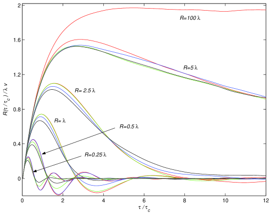
Figure 1: The position-velocity correlation function, $R\left(\tau\right)=2h\left(\tau\right)$ as a function of cell radius $R$ parameterized in terms of the mean free path $\lambda$ for different degrees of specularity as parameterized by the angular spread of the final angle compared to the incident angle. Red: specular; Green: $45^{\circ}$; Blue: $90^{\circ}$; Black: diffuse. For $R\gtrsim 2.5\lambda$, there was practically no effect due to the degree of specularity, as expected.

Results of a two-dimensional Monte Carlo calculation are shown in Figure 1. Taking $\lambda=1$ and fixed, we see the effect of wall collisions as the bottle radius approaches $\lambda$. We see in Fig. 1 that in all cases $R(\tau)$ initially increases linearly. The effect of the wall collisions when $R>\lambda$ is to limit the distance that the random walk can take, and this appears as an exponential decay in $R\left(\tau\right)$ at long times. This effect does not depend on the specularity of the wall collisions and is best seen as an effect on the whole ensemble of particles which can be described by classical diffusion theory. In this limit, the correlation function is well-described by

$$R(\tau)=(1-e^{-\tau/\tau_{c}})e^{-\tau/T}$$ (46)

where, from analysis of the plots,

$$T\approx{\frac{0.6R^{2}}{\lambda v}}.$$ (47)

In the other limit, $R<\lambda$, $R(\tau)$ oscillates with frequency

$$\omega\approx{\frac{2\pi v}{5.2R}}$$ (48)

and

$$R(\tau)=e^{-\tau/T}\sin\omega\tau$$ (49)

where $T$ depends on $\Delta\theta$, but is typically of order $2\pi/\omega$.

The frequency shift is determined by Eq. (26) and in the case of large $R$ we find ($\tau_{c}<<T$), using Eq. (47)

$$\delta\omega={\frac{abR^{2}}{T^{2}\omega_{0}^{2}+1}}={\frac{abR^{2}}{1+(0.6R^{2}\omega_{0}/v\lambda)^{2}}}.$$ (50)

These results are in good agreement with JMP , Fig. 10, for which $4/2\pi\approx 0.634$ replaces the factor $0.6$ above and with Eq. (75) below.

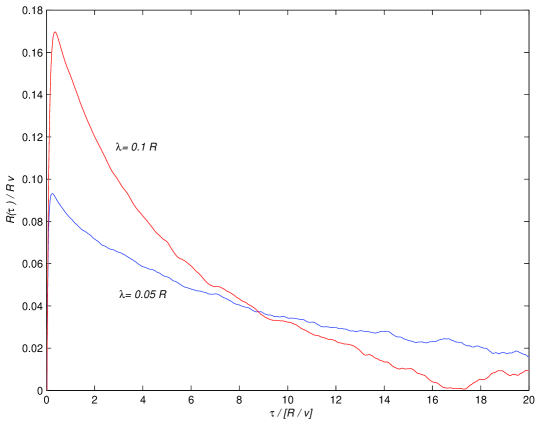
Figure 2: The position-velocity correlation function when $\lambda$ is very small. This represents the limit for slow diffusion.

Additional insight can be gained by considering the effects of varying $\lambda$ keeping $R$ fixed, as shown in Fig. 2 for very small $\lambda$. In this limit, the horizontal axis is multiplied by $\lambda/R$ to define time proportional to $R/v$. The correlation amplitude function is proportional to $\lambda v$ and the decaying exponential time constant is

$$T\propto{\frac{R^{2}}{\lambda v}}.$$ (51)

The time to reach the peak value is

$$\tau_{0}\propto\lambda^{2}/Rv$$ (52)

which approaches zero as $R\rightarrow\infty$.

This limit is further discussed in Sec. 4.1, and the frequency shift in this case is in general agreement with Fig. 10 of JMP .

The curves for large (relative to $R$) $\lambda$ in figure 1 show damped oscillations whose damping depends on the angular spread of the wall collisions. This is a manifestation of the resonance behavior discussed in ref. JMP for the case of perfectly specular wall collisions. Here we see the damping due to non-specular reflections.

II.2 Numerical estimations of the frequency shift for all values of $\omega_{o}/\omega_{r}$

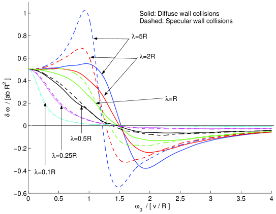
Figure 3: Results of numerically applying Eq. (37) to numerical calculations of the correlation function, for varying $\lambda$ with $R$ fixed.

Using Eq. (37), and the results of the previous section, the cosine transform of the numerically-determined correlation function can be calculated numerically. In order to reduce oscillations due to the finite time window, a Hamming window function was applied to the correlation function, and a slight correction due to the frequency dependent gain as imposed by the window function was applied. The results, as a function of mean free path $\lambda$ at fixed radius $R$, for specular and purely diffuse wall reflection, are shown in Fig. 3.

There are a few points worth noting. First, the curves for large $\lambda$ in the specular case are very similar to the Bloch-Siegert result. Second, at small and large frequencies, the results agree with the numerical semi-analytically determined results presented above, and in JMP and the theoretical analysis below. Third, the behavior at intermediate frequencies is seen to be very interesting: The shift goes to zero for $\omega_{o}/\omega_{r}\sim 1$ as it must because the effect changes sign between large and small frequencies.

Furthermore, it can be seen immediately that the effects of wall collision specularity is important when $\omega_{o}\approx\omega_{r}$, in contradiction to the statement in JMP that the degree of specularity does not affect the frequency shift. We discuss this point later in more detail (Sec. IV).

III Analytical results for the limiting cases of large and small frequencies $(\omega_{o}/\omega_{r}\gg 1,\omega_{o}/\omega_{r}\ll 1)$

Equation (43 ) represents the formal solution of the problem in all cases of interest here. Thus the frequency shift is determined entirely by the velocity auto-correlation function of the particles undergoing magnetic resonance. This function has been the subject of intense experimental and theoretical study (Egelstaff ; Lovesey ; squires ). In our case, involving macroscopic distances and times, it suffices to treat the motion classically. For relatively short times if the particles undergo collisions which are distributed according to a Poisson distribution with average time between collisions given by $\tau_{c}$, the velocity correlation function is well known to be given by

$$\psi\left(t\right)=\left\langle v^{2}\right\rangle e^{-t/\tau_{c}}$$ (53)

This form is known to be valid for relatively short times. According to Eq. (37) the frequency shift depends on the Fourier transform of the integral of the velocity correlation function evaluated at $\omega_{o}$. So the short time behavior of $\psi\left(t\right)$ determines the high frequency behavior of $\psi\left(\omega\right)$, and the result using this form is expected be valid in the case of large $\omega_{o}$, i.e. $\omega_{o}\gg\omega_{r}$.

For longer times the velocity correlation function is well described by classical diffusion theory. Thus the long time behavior will determine the low frequency region of the velocity spectrum and the result will apply to the case $\omega_{o}\ll\omega_{r}$. In this region the result will depend on the size of the containing vessel as the dynamics of the diffusion process are influenced by the boundary conditions.

III.1 Short correlation times ($\omega_{r}\ll\omega_{o}$)

Using (53) we have

$$\psi\left(\omega\right)=\frac{1}{\pi}\left\langle v^{2}\right\rangle\int_{0}^{\infty}\cos\omega te^{-t/\tau}dt=\frac{1}{\pi}\left\langle v^{2}\right\rangle\frac{1}{\tau\left(\omega^{2}+\frac{1}{\tau^{2}}\right)}$$ (54)

so that according to (43)

$$\delta\omega =-ab\int_{-\infty}^{\infty}\frac{\psi(\omega)}{\left(\omega_{o}^{2}-\omega^{2}\right)}d\omega$$ (55)

$$=ab\frac{1}{\pi}\frac{\left\langle v^{2}\right\rangle}{\tau}\int_{-\infty}^{\infty}\frac{1}{\left(\omega^{2}+\frac{1}{\tau^{2}}\right)\left(\omega^{2}-\omega_{o}^{2}\right)}d\omega$$ (56)

$$=-ab\frac{\left\langle v^{2}\right\rangle}{\omega_{o}^{2}}\frac{1}{\left(1+\frac{1}{\omega_{o}^{2}\tau^{2}}\right)}$$ (57)

This is in substantial agreement with  the expression given in the caption of JMP Fig. 12 when it is taken with JMP Eq. (19) or (3) applicable to the case when $\omega_{r}\ll\omega_{o}$. It is quite likely that the small discrepancy ($\sim 10\%$) in the 50% suppression point is due to the process of averaging over the velocity distribution in JMP Fig. 12.

III.2 Diffusion theory calculation of the long time behavior of the velocity correlation function. Frequency shifts for ($\omega_{r}\gg\omega_{o}$)

Whereas the previous case applies to UCN this case would apply to atoms used as a comagnetometer and is more relevant experimentally as it results in larger shifts JMP and in some cases RPPedm the collision rate can be simply adjusted by changing the experimental conditions.

In the following we review the solution of the diffusion equation in cylindrical geometry, obtain the velocity autocorrelation function from the solution and calculate the frequency shift. In the limit of small collision rate the result agrees with the known results for ($\omega_{r}\gg\omega_{o}$) and the effect of the collisions agrees with that found from numerical simulations (JMP Fig. 10)

III.2.1 Green’s function for the diffusion equation in cylindrical geometry

In this section we attempt to understand the effects of the vessel boundary on the velocity autocorrelation function, observed in the numerical simulations (section II.1), by  applying classical diffusion theory to the problem. Diffusion theory is expected to be valid for long times so that we expect the results to be valid for small $\omega_{o}$, i.e. $\omega_{o}\ll\omega_{r}$.

$$D\nabla^{2}\rho-\frac{\partial\rho}{\partial t} =0$$

$$\rho =u_{k}(r)e^{-Dk^{2}t}$$

$$\nabla^{2}u+k^{2}u =0$$ (58)

We consider a two dimensional problem, that is we neglect any $z$ dependence $\left(k_{z}=0\right).$ For the cases considered in JMP where the height of the bottle is much smaller than the radius higher $z$ modes will decay relatively quickly.

The boundary condition is $j\left(R\right)=-D\frac{\partial\rho}{\partial r}=0$ so the eigenfunctions satisfying the boundary conditions are

$$u_{m,n} =N_{m,n}J_{m}(k_{m,n}r)e^{im\theta}$$

$$k_{m,n}R =x_{m,n}^{\prime}\text{ (}n^{th}\text{ zero of }dJ_{m}(z)/dz\text{)}$$

where the normalization constant (which depends on the boundary conditions) is (Sommerfeld , p 322)

$$N_{m,n}=\frac{1}{\sqrt{2\pi}J_{m}(k_{m,n}R)}\sqrt{\frac{2k_{m,n}^{2}}{\left(k_{m,n}R\right)^{2}-m^{2}}}$$ (59)

The Greens’ function satisfying the boundary conditions is morsefesh

$$G(r,r^{\prime},t)=\sum_{m,n}\left(N_{m,n}\right)^{2}J_{m}(k_{m,n}r)J_{m}(k_{m,n}r^{\prime})e^{im\left(\theta-\theta^{\prime}\right)}e^{-Dk_{m,n}^{2}t}$$ (60)

This is the probability of finding a particle at $\overrightarrow{r}$ at time $t$, given that the particle was at $\overrightarrow{r}^{\prime}$ at time $t=0$. The spectrum of the velocity correlation function is related to $S\left(\overrightarrow{q},\omega\right)$ which in turn is the average over the system of the Fourier transform of this probability with respect to $\rho=\left(r-r^{\prime}\right)$. We use the cosine transform because we want the cosine transform of the velocity correlation function (38) $\psi\left(\omega\right)$.

$$S(q,\omega) =\frac{1}{\pi}\left\langle\int d^{2}\rho e^{i\overrightarrow{q}\cdot\overrightarrow{\rho}}\int_{0}^{\infty}dt\cos\omega tG(r,r^{\prime},t)\right\rangle$$ (61)

$$=\frac{1}{\pi}\int\int\frac{d^{2}r^{\prime}}{\pi R^{2}}d^{2}\rho e^{i\overrightarrow{q}\cdot\overrightarrow{\rho}}\int_{0}^{\infty}dt\cos\omega tG(r,r^{\prime},t)$$ (62)

$$=\frac{1}{\pi^{2}R^{2}}\sum_{m,n}\left(N_{m,n}\right)^{2}\int d^{2}re^{i\overrightarrow{q}\cdot\overrightarrow{r}}J_{m}(k_{m,n}r)e^{im\theta}\times$$ (63)

$$\int d^{2}r^{\prime}e^{-i\overrightarrow{q}\cdot\overrightarrow{r}^{\prime}}J_{m}(k_{m,n}r^{\prime})e^{-im\theta^{\prime}}\frac{Dk_{m,n}^{2}}{\omega^{2}+\left(Dk_{m,n}^{2}\right)^{2}}$$ (64)

Now we can evaluate the integrals using

$$J_{m}\left(x\right)=\frac{\left(-i\right)^{m}}{2\pi}\int_{0}^{2\pi}e^{i\left(x\cos\theta+m\theta\right)}d\theta$$ (65)

and Bessel function identities

$$\int d^{2}re^{i\overrightarrow{q}\cdot\overrightarrow{r}}J_{m}(k_{m,n}r)e^{im\theta} =\frac{2\pi\left(i\right)^{\pm m}}{\left(q^{2}-k_{m,n}^{2}\right)}\frac{qR}{2}J_{m}(k_{m,n}R)\times$$

$$\left[J_{m-1}(qR)-J_{m+1}(qR)\right]$$

thus

$$S(q,\omega) =\frac{2}{\pi^{3}R^{2}}\sum_{m,n}..$$ (66)

$$\frac{k_{m,n}^{2}}{\left(\left(k_{m,n}R\right)^{2}-m^{2}\right)}\left(\frac{2\pi}{\left(q^{2}-k_{m,n}^{2}\right)}\frac{qR}{2}\left[J_{m-1}(qR)-J_{m+1}(qR)\right]\right)^{2}\frac{Dk_{m,n}^{2}}{\left(\omega^{2}+\left(Dk_{m,n}^{2}\right)^{2}\right)}$$ (67)

III.2.2 Velocity autocorrelation function

The velocity autocorrelation function

$$\psi(\tau)=\left\langle\overrightarrow{v}\left(0\right)\cdot\overrightarrow{v}\left(\tau\right)\right\rangle$$ (68)

has a Fourier transform given by (degenn )

$$\psi\left(\omega\right)=\lim_{q\rightarrow 0}2\left(\frac{\omega}{q}\right)^{2}S(q,\omega)$$ (69)

so that the only terms in (67) which contribute are those containing $J_{0}\left(qR\right)$, since $\lim_{x\rightarrow 0}J_{n}\left(x\right)\thicksim\left(x\right)^{n}$, $J_{0}\left(0\right)=1.$ Thus we only need to keep terms with $m=\pm 1$ in (67) and we find

$$\lim_{q\rightarrow 0}S(q,\omega)=\frac{2q^{2}}{\pi\left(\left(k_{1,n}R\right)^{2}-1\right)}\frac{D}{\left(\omega^{2}+\left(Dk_{1,n}^{2}\right)^{2}\right)}$$ (70)

Then

$$\psi\left(\omega\right)=\frac{1}{\pi}\sum_{n}\frac{4}{\left(x_{1,n}^{2}-1\right)}\frac{D\omega^{2}}{\left(\omega^{2}+\left(Dk_{1,n}^{2}\right)^{2}\right)}$$ (71)

III.2.3 Frequency shift in the diffusion approximation (cylindrical geometry)

According to (43)

$$\delta\omega =-ab\int_{-\infty}^{\infty}\psi(\omega)\frac{1}{\omega_{o}^{2}-\omega^{2}}d\omega$$ (72)

$$=abR^{2}\sum_{n}\frac{4}{\left(x_{1,n}^{2}-1\right)}\frac{1}{x_{1,n}^{2}\left(\left(\frac{\omega_{o}R^{2}}{Dx_{1,n}^{2}}\right)^{2}+1\right)}$$ (73)

The result (73) is dominated by the first mode $x_{1,1}=1.84$. Figure 3 shows the first term in comparison to the sum of the first 4 terms. For convenience we list the zeroes of $J_{1}^{\prime}(x)$: $x_{1,2}=5.33,x_{1,3}=8.54,x_{1,4}=11.7$. Since we are dealing with a 2 dimensional problem we put

$$D=v^{2}\tau/2$$ (74)

(instead of $\tau v^{2}/3$ for 3 dimensions) in order to facilitate the comparison with the numerical simulations JMP and obtain for the condition that the frequency shift is reduced to 50% of its value in the absence of collisions

$$\eta=\frac{\omega_{o}R^{2}}{Dx_{1,n}^{2}}=\frac{2\omega_{o}R^{2}}{v^{2}\tau x_{1,n}^{2}}=.59\frac{\omega_{o}R^{2}}{v^{2}\tau}=1$$ (75)

the numerical factor of which is to be compared with $\frac{2}{\pi}=.634$ obtained in [JMP ], fig. 10 by fitting simulated results, and our numerical result of $0.6$ presented in Sec. II.1. The magnitude $abR^{2}/2$ of (73) in the absence of collisions is just that expected from the Bloch-Siegert treatment in the case $\omega_{r}\gg\omega_{o}$ (Eq. (3), JMP Eq. (21)), averaged over the different trajectories as discussed in JMP after equation (22).

III.2.4 Frequency shift in the diffusion approximation (rectangular geometry)

For the rectangular case the normalized eigenfunctions are

$$u_{m,n}\left(x,y\right)=\sqrt{\frac{2}{L_{x}}}\cos\frac{m\pi}{L_{x}}x\sqrt{\frac{2}{L_{y}}}\cos\frac{m\pi}{L_{y}}y$$ (76)

which satisfy the reflection boundary conditions at $x=0,L_{x}$ and $y=0,L_{y}$. For $n$ or $m=0$ the corresponding eigenfunctions are

$$u_{0}=\frac{1}{\sqrt{L_{x,y}}}$$ (77)

so that the Green’s function is

$$G(x,x^{\prime},y,y^{\prime},t) =\sum_{m,n=0}^{\infty}\left[\frac{1}{L_{x}}+\frac{2}{L_{x}}\cos k_{m}x\cos k_{m}x^{\prime}e^{-Dk_{m}^{2}t}\right]\times$$

$$\left[\frac{1}{L_{y}}+\frac{2}{L_{y}}\cos k_{n}x\cos k_{n}x^{\prime}e^{-Dk_{n}^{2}t}\right]$$ (78)

with $k_{m,n}=\left(m,n\right)\pi/L_{x,y}$. To calculate $\lim_{q\rightarrow 0}S\left(q,\omega\right)$ we need integrals of the form

$$\lim_{q\rightarrow 0}\int_{0}^{L}e^{iq_{x}x}\cos k_{m}xdx =\frac{q_{x}}{q_{x}^{2}-k_{m}^{2}}\left\{\begin{array}[c]{cc}q_{x}L_{x}&m=2,4,6..\\ \frac{-2}{i}&m=1,3,5..\end{array}\right\}$$ (81)

$$=\left\{\begin{array}[c]{cc}L_{x}&m=0\end{array}\right\}$$ (83)

Since each of these will appear squared because of the contribution from the $x,x^{\prime}$ integrals we can only take the odd values of $m$. The even numbers will yield a higher power of $q$ which will vanish in the limit. Given this, if we take $m=1,3,5$ we must take $n=0$ and vice-versa. We calculate, using (81)

$$\lim_{q\rightarrow 0}\left[S\left(q,\omega\right)=\int dx\int\frac{dx^{\prime}}{L_{x}}\int dy\int\frac{dy^{\prime}}{L_{y}}e^{i\overrightarrow{q}\cdot\left(\overrightarrow{x}-\overrightarrow{x}^{\prime}\right)}\frac{1}{\pi}\int_{0}^{\infty}dt\cos\omega tG\left(\overrightarrow{x},\overrightarrow{x}^{\prime},t\right)\right]$$ (84)

$$=q^{2}\frac{8}{2\pi}\left(\begin{array}[c]{c}\sum_{m=1,3,5..}\frac{1}{k_{m}^{2}\left(m\pi\right)^{2}}\frac{Dk_{m}^{2}}{\omega^{2}+\left(Dk_{m}^{2}\right)^{2}}+\\ \sum_{n=1,3,5..}\frac{1}{k_{n}^{2}\left(n\pi\right)^{2}}\frac{Dk_{n}^{2}}{\omega^{2}+\left(Dk_{n}^{2}\right)^{2}}\end{array}\right)$$ (87)

where we used $\left\langle q_{x}^{2}\right\rangle=\left\langle q_{y}^{2}\right\rangle=q^{2}/2$. Then

$$\psi\left(\omega\right)=\frac{8\omega^{2}}{\pi}\left(\sum_{m=1,3,5..}\frac{1}{k_{m}^{2}\left(m\pi\right)^{2}}\frac{Dk_{m}^{2}}{\omega^{2}+\left(Dk_{m}^{2}\right)^{2}}+\sum_{n=1,3,5..}\frac{1}{k_{n}^{2}\left(n\pi\right)^{2}}\frac{Dk_{n}^{2}}{\omega^{2}+\left(Dk_{n}^{2}\right)^{2}}\right)$$ (88)

and (using 43)

$$\delta\omega =-ab\int_{-\infty}^{\infty}\psi(\omega)\frac{1}{\omega_{o}^{2}-\omega^{2}}d\omega$$ (89)

$$=8ab\left(\sum_{m=1,3,5..}\frac{L_{x}^{2}}{\left(m\pi\right)^{4}}\frac{1}{\left(\frac{\omega_{o}L_{x}^{2}}{D\left(m\pi\right)^{2}}\right)^{2}+1}+\sum_{n=1,3,5..}\frac{L_{y}^{2}}{\left(n\pi\right)^{4}}\frac{1}{\left(\frac{\omega_{o}L_{y}^{2}}{D\left(n\pi\right)^{2}}\right)^{2}+1}\right)$$ (90)

We thus see that in a rectangular box $L_{x}\neq L_{y}$ it is the longer side which dominates the behavior.

III.3 Diffusion theory calculation of the long time behavior of the velocity correlation function. Frequency shifts for ($\omega_{r}\gg\omega_{o}$) (Alternate caclulation)

In this section we derive the diffusion theory result for cylindrical geometry (73) using an alternate method based on that of Mcgregor McGregor which avoids the use of the theorem (69). We start with the Green’s function for cylindrical geometry given above (60)

$$G(r,r^{\prime},t)=\sum_{m,n}\left(N_{m,n}\right)^{2}J_{m}(k_{m,n}r)J_{m}(k_{m,n}r^{\prime})e^{im\left(\phi-\phi^{\prime}\right)}e^{-Dk_{m,n}^{2}t}$$ (91)

This is the probability of finding a particle at $\overrightarrow{r}$ at time $t$, given that the particle was at $\overrightarrow{r}^{\prime}$ at time $t=0$.

III.3.1 Position-velocity correlation function $R(\tau)$

From equ. (27) we have

$$R(\tau) =\left\langle y(t)v_{y}(t-\tau)+x(t)v_{x}(t-\tau)-y(t-\tau)v_{y}(t)-x(t-\tau)v_{x}(t)\right\rangle$$ (92)

$$=\left\langle\overrightarrow{r}(t)\cdot\overrightarrow{v}(t-\tau)-\overrightarrow{r}(t-\tau)\cdot\overrightarrow{v}(t\right\rangle=\left|\frac{d}{dt^{\prime}}\left\langle\overrightarrow{r}(t)\cdot\overrightarrow{r}(t\prime)\right\rangle-\frac{d}{dt}\left\langle\overrightarrow{r}(t\prime)\cdot\overrightarrow{r}(t)\right\rangle\right|_{t^{\prime}=t-\tau}$$ (93)

Following McGregor McGregor we write

$$\left\langle\overrightarrow{r}(t)\cdot\overrightarrow{r}(t\prime)\right\rangle =\int d^{2}r\int\frac{d^{2}r^{\prime}}{\pi R^{2}}G(r,r^{\prime},t-t^{\prime})\left\langle\overrightarrow{r}\cdot\overrightarrow{r^{\prime}}\right\rangle$$ (94)

$$=\frac{1}{\pi R^{2}}\sum_{m,n}\left(N_{m,n}\right)^{2}\int rdrd\phi J_{m}(k_{m,n}r)\int r^{\prime}dr^{\prime}d\phi^{\prime}J_{m}(k_{m,n}r^{\prime})\times$$ (95)

$$\times rr^{\prime}e^{im\left(\phi-\phi^{\prime}\right)}\left[\cos\phi\cos\phi^{\prime}+\sin\phi\sin\phi^{\prime}\right]e^{-Dk_{m,n}^{2}\left(t-t^{\prime}\right)}$$ (96)

Since $\left(N_{m,n}\right)^{2}=\left(N_{-m,n}\right)^{2}$ and $J_{-m}(z)=(-1)^{m}J_{m}(z),$ (59) we can (excluding $m=0$, which will be seen not contribute to the result) combine the terms for $m$ and $-m$ as follows:

$$\left\langle\overrightarrow{r}(t)\cdot\overrightarrow{r}(t\prime)\right\rangle =\frac{1}{\pi R^{2}}\sum_{m>0,n}\left(N_{m,n}\right)^{2}\int r^{2}drJ_{m}(k_{m,n}r)\int r^{\prime^{2}}dr^{\prime}J_{m}(k_{m,n}r^{\prime})\times$$ (97)

$$\times\int d\phi\int d\phi^{\prime}\Xi(\phi,\phi^{\prime})e^{-Dk_{m,n}^{2}\left(t-t^{\prime}\right)}$$ (98)

where

$$\Xi(\phi,\phi^{\prime}) =\left[\cos\phi\cos\phi^{\prime}+\sin\phi\sin\phi^{\prime}\right]2\cos m\left(\phi-\phi^{\prime}\right)$$ (99)

$$=2\left[\cos\phi\cos\phi^{\prime}+\sin\phi\sin\phi^{\prime}\right]\left[\cos m\phi\cos m\phi^{\prime}+\sin m\phi\sin m\phi^{\prime}\right]$$ (100)

$$=\frac{1}{2}\left(\cos\phi\cos m\phi\cos\phi^{\prime}\cos m\phi^{\prime}+\sin\phi\sin m\phi\sin\phi^{\prime}\sin m\phi^{\prime}+\right.$$ (101)

$$\left.+\sin\phi\cos m\phi\sin\phi^{\prime}\cos m\phi^{\prime}+\cos\phi\sin m\phi\cos\phi^{\prime}\sin m\phi^{\prime}\right)$$ (102)

$$=\frac{1}{2}\left[\left(\cos\left(m-1\right)\phi+\cos\left(m+1\right)\phi\right)\left(\cos\left(m-1\right)\phi^{\prime}+\cos\left(m+1\right)\phi^{\prime}\right)+\right.$$ (103)

$$+\left(\cos\left(m-1\right)\phi-\cos\left(m+1\right)\phi\right)\left(\cos\left(m-1\right)\phi^{\prime}-\cos\left(m+1\right)\phi^{\prime}\right)+$$ (104)

$$+\left(\sin\left(m-1\right)\phi-\sin\left(m+1\right)\phi\right)\left(\sin\left(m-1\right)\phi^{\prime}-\sin\left(m+1\right)\phi^{\prime}\right)+$$ (105)

$$+\left(\sin\left(m-1\right)\phi+\sin\left(m+1\right)\phi\right)\left(\sin\left(m-1\right)\phi^{\prime}+\sin\left(m+1\right)\phi^{\prime}\right)$$ (106)

using

$$\int_{0}^{2\pi}d\phi\cos(m+1)\phi =0\quad(m>0),\quad\int_{0}^{2\pi}d\phi\sin(m\pm 1)\phi=0$$ (107)

$$\int_{0}^{2\pi}d\phi\cos(m-1)\phi =2\pi\delta_{m1}$$ (108)

we have

$$\int d\phi\int d\phi^{\prime}\Xi(\phi,\phi^{\prime})=\frac{\left(2\pi\right)^{2}}{2}2\delta_{m1}$$ (109)

so that

$$\left\langle\overrightarrow{r}(t)\cdot\overrightarrow{r}(t\prime)\right\rangle =\frac{1}{\pi R^{2}}\left(2\pi\right)^{2}\sum_{m>0,n}\delta_{m1}\left(N_{m,n}\right)^{2}\int r^{2}drJ_{m}(k_{m,n}r)\int r^{\prime^{2}}dr^{\prime}J_{m}(k_{m,n}r^{\prime})e^{-Dk_{m,n}^{2}\left(t-t^{\prime}\right)}$$ (110)

$$=\frac{4\pi}{R^{2}}\sum_{n}\left(N_{1,n}\right)^{2}\int_{0}^{R}r^{2}drJ_{1}(k_{1,n}r)\int_{0}^{R}r^{\prime^{2}}dr^{\prime}J_{1}(k_{1,n}r^{\prime})e^{-Dk_{1,n}^{2}\left(t-t^{\prime}\right)}$$ (111)

Using

$$\int_{0}^{\alpha}z^{n}dzJ_{n-1}(z) =\left[z^{n}J_{n}(z)\right]_{0}^{\alpha}$$ (112)

$$J_{n}^{\prime}(z) =\frac{n}{z}J_{n}(z)-J_{n+1}(z)$$ (113)

we have

$$\int_{0}^{R}r^{2}drJ_{1}(k_{1,n}r)=\frac{R^{3}}{\left(x_{1,n}^{\prime}\right)^{2}}J_{1}(x_{1,n}^{\prime})$$ (114)

Thus

$$\left\langle\overrightarrow{r}(t)\cdot\overrightarrow{r}(t\prime)\right\rangle =\frac{4\pi}{R^{2}}\sum_{n}\left(N_{1,n}\right)^{2}\frac{R^{6}}{\left(x_{1,n}^{\prime}\right)^{4}}J_{1}^{2}(x_{1,n}^{\prime})e^{-Dk_{1,n}^{2}\left(t-t^{\prime}\right)}$$ (115)

$$=4R^{2}\sum_{n}\frac{1}{\left(x_{1,n}^{\prime}\right)^{2}\left(\left(x_{1,n}^{\prime}\right)^{2}-1\right)}e^{-Dk_{1,n}^{2}\left(t-t^{\prime}\right)}$$ (116)

$$=\sum_{n}\eta_{n}e^{-Dk_{1,n}^{2}\left(t-t^{\prime}\right)}$$ (117)

and

$$R\left(\tau\right)=2\sum_{n}\eta_{n}Dk_{1,n}^{2}e^{-Dk_{1,n}^{2}\tau}$$ (118)

using (93). Then according to (26)

$$\delta\omega =\frac{ab}{2}\int_{0}^{t}d\tau\left(\cos\omega_{o}\tau\right)R\left(\tau\right)$$ (119)

$$=ab\int_{0}^{t}d\tau\left(\cos\omega_{o}\tau\right)\sum_{n}\eta_{n}Dk_{1,n}^{2}e^{-Dk_{1,n}^{2}\tau}$$ (120)

$$=4abR^{2}\sum_{n}\frac{1}{\left(x_{1,n}^{\prime}\right)^{2}\left[\left(x_{1,n}^{\prime}\right)^{2}-1\right]}\frac{1}{\left[\left(\frac{\omega_{o}R^{2}}{Dx_{1,n}^{\prime 2}}\right)^{2}+1\right]}$$ (121)

in complete agreement with equation (73).

III.4
Application: ³He Comagnetometer

In RPPedm the use of ³He as a comagnetometer for a UCN neutron EDM experiment is discussed. This system is rather unique in that an effective background gas (phonons) can be introduced which affects the ³He significantly while having no substantial interaction with the UCN for temperatures below 0.5 K. Because the ³He and neutron magnetic moments are equal to within 10%, it is possible to control this systematic by varying the size of the effect for ³He by changing the diffusion rate of the ³He.

The UCN upscattering lifetime varies as $100T^{-7}$ s for $T<0.7$ K, while the coefficient of diffusion for ³He in a superfluid helium bath varies as $D\approx 1.6T^{-7}$ cm²/s diffusion .

In connection with (75) this yields $\eta=1$ when the superfluid helium temperature is $T\approx 0.25$ K, (R=25cm), which determines the temperature scale where the effect can be varied, and is within the design range of operating temperature for the planned experiment, compatible with a UCN upscattering lifetime in excess of 1000 s.

IV Discussion

One of the surprising, but unexplained results of JMP was that according to their numerical simulations, wall collisions had no influence on the magnitude of the frequency shifts while gas collisions could eliminate the frequency shifts completely if their rate is high enough. This was apparently only studied in the limits of large and small $\omega_{o}/\omega_{r}.$ We now know that this does not apply to intermediate frequencies, e.g, when $\omega_{o}\sim\omega_{r}$. In Fig. 3 we see that wall collisions have a serious influence at intermediate frequencies when $\lambda\geq R$. Also from Fig. 3 we see that the curves for diffuse wall reflections in the absence of gas collisions is very similar to the specular curves for $\lambda<R/2$. This implies that there is no essential difference between wall and gas collisions. We now show that the reason the wall collisions have no effect at the limiting frequencies, contrary to the case at intermediate frequencies, is that the wall collisions are never fast enough to influence the systematic (proportional to $\overrightarrow{E})$ frequency shifts in the limits of large and small $\omega_{o}$.

For a particles in a cylindrical vessel following a trajectory along a chord subtending an angle $2\alpha$, the time between collisions is

$$\tau_{c}=\frac{2R}{v}\sin\alpha$$ (122)

and the effective field rotation frequency is given by

$$\omega_{r}=2\alpha/\tau_{c}=\frac{\alpha v}{R\sin\alpha}$$ (123)

Considering first the case when $\omega_{r}\gg\omega_{o}$ (73,JMP Fig. 10,) the systematic frequency shift was found to be suppressed by the factor $\eta$

$$\eta =\frac{1}{1+\beta^{2}}$$

$$\beta =\frac{2R^{2}\omega_{o}}{\pi v^{2}\tau_{c}}$$

For significant suppression we need $\beta\gtrsim 1$

$$\frac{2R^{2}\omega_{o}}{\pi v^{2}\tau_{c}} =\frac{R\omega_{o}}{\pi v\sin\alpha}\gtrsim 1$$ (124)

$$\sin\alpha \lesssim\frac{R\omega_{o}}{\pi v}=\frac{25\times 2\cdot 7}{10^{4}}\sim\frac{1}{30}$$

for representative conditions in JMP , fig. 10. ($R=25,B_{o}=1\mu T,v=10^{4}cm/\sec$).

The probability of a given value of $\alpha$ is given in Eq. (B1) of JMP as

$$P(\alpha)d\alpha =\frac{4}{\pi}\sin^{2}\alpha d\alpha$$ (125)

$$P(\alpha \leq\varepsilon)\sim\varepsilon^{3}$$

so that the wall collisions would only be expected to be effective for a vanishingly small fraction of the trajectories.

Turning now to the case $\omega_{r}\ll\omega_{o}$ (57, Fig. 12 of JMP ) we have as the condition that the suppression be effective:

$$\beta =\frac{1}{\omega_{o}\tau_{c}}\geq 1$$

$$\frac{1}{\omega_{o}} \gtrsim\frac{2R}{v}\sin\alpha$$

$$\sin\alpha \leq\frac{v}{2R\omega_{o}}=\frac{200}{2\cdot 25\cdot 200}=\frac{1}{50}$$

for conditions typical of JMP Fig. 12 ($v=200cm/\sec,B_{o}=1\mu T$).

Thus the wall collisions rate is never high enough to significantly effect the magnitude of the frequency shift at the limits. The wall collisions do, however, broaden and shift the resonances discussed in JMP

V Conclusion

We have developed a general technique of analyzing the systematic effects due to a combination of an electric field and magnetic gradients as encountered in EDM experiments that employ gasses of stored particles. Use of the correlation technique, either by numerical calculations for complicated geometries, or by the velocity correlation function for simpler geometries, provides a simplified approach to the problem compared to numerical integration of the Bloch equations. Our analysis has added insight to this new systematic effect and provides a means of rapidly assessing the effects of various geometries and angular distributions for wall and gas collisions.

VI Acknowledgements

We are grateful to Werner Heil and Yuri Sobolev for calling our attention to this problem and to George Jackeli and Boris Toperverg for an enlightening conversation. We also thank J.M. Pendlebury et al. for providing a draft of their manuscript before publication.

VII Appendix 1: Matrix algebra of spherical Pauli matrices

The following relationships among the Pauli matrices have been employed in the calculation in section I.1.

$$2\sigma_{\pm}=\sigma_{x}\pm i\sigma_{y}$$ (126)

$$\sigma_{\pm}\sigma_{z}=\mp\sigma_{\pm};\ \ \ \sigma_{z}\sigma_{\pm}=\sigma_{\pm}$$ (127)

$$\sigma_{\pm}\sigma_{\mp}={\frac{1}{2}}\pm{\frac{1}{2}}\sigma_{z}$$ (128)

$$\sigma_{z}\sigma_{z}=1;\ \ \ \sigma_{\pm}\sigma_{\pm}=0$$ (129)

VIII Appendix 2: Egelstaff’s velocity correlation function theorem; a new look at an old theorem

VIII.1 Introduction

The relation between the velocity autocorrelation function (vacf) and $S_{s}\left(q,\omega\right)$ which we used in section [III.2] was first introduced by Egelstaff Egelstaff2 and has proven to be a useful tool in the study of liquids. The vacf can be simulated for various models and obtained from neutron scattering data using Egelstaff’s theorem. The theorem has been discussed by several authors Egelstaff , Lovesey , squires and has been given in slightly different forms depending on the normalization chosen for the functions involved.

Following Squires’ squires derivation would yield

$$\psi(\omega)=3\omega^{2}\lim_{q\rightarrow 0}\frac{S_{inc}(q,\omega)}{q^{2}}$$ (130)

if we were to define

$$\psi(\omega)=\frac{1}{2\pi}\int_{-\infty}^{\infty}\left\langle\overrightarrow{v}(0)\cdot\overrightarrow{v}(\tau)\right\rangle e^{-i\omega\tau}d\tau$$

which has a different normalization then used by Squires. Egelstaff gives the theorem as

$$\psi(\omega)=\omega^{2}\left[\frac{S_{inc}(q,\omega)}{q^{2}}\right]_{q\rightarrow 0}$$

where he defines

$$\psi(\omega)=\frac{1}{2\pi}\int_{-\infty}^{\infty}\left\langle v_{x}(0)\cdot v_{x}(\tau)\right\rangle e^{-i\omega\tau}d\tau$$

which accounts for the factor of 3 difference. Both authors give the derivation only for the Gaussian approximation where we take

$$G(\overrightarrow{r},t) =\frac{1}{\left(2\pi w(\tau)\right)^{3/2}}e^{-\frac{{}^{r^{2}}}{2w(\tau)}}$$

$$I(q,\tau) =\int d^{3}rG(\overrightarrow{r},t)e^{i\overrightarrow{q}\cdot\overrightarrow{r}}=e^{-q^{2}\frac{w(\tau)}{2}}$$ (131)

Boon and Yip boyip derive the theorem for the general case, i.e. without the Gaussian approximation.

The theorem has been used to extract vacf’s from neutron scattering data by many authors. An early example is given by Egelstaff2 . See also the work of Carneiro carneiro .

The fact that sections III.2 and III.3 give the same result and section III.2 uses Egelstaff’s theorem while section III.3 does not, suggests that we have discovered a new way of proving the theorem.

VIII.2 A new derivation of Egelstaff’s theorem

In this section we will give a general derivation (not relying on the Gaussian approximation) of Egelstaff’s theorem.

We begin by following the formulation of Squires squires and calculate the velocity autocorrelation function

$$\psi(\tau)=\left\langle\overrightarrow{v}(0)\cdot\overrightarrow{v}(\tau)\right\rangle$$

as follows:

Let $\overrightarrow{r}(t)$ be the position of a particle at time $t$, when the particle was at the position $\overrightarrow{r}(0)$ at time $t=0$. Then

$$r(t) \triangleq\overrightarrow{r}(t)-\overrightarrow{r}(0)=\int_{0}^{t}\overrightarrow{v}(t^{\prime})dt^{\prime}$$

$$r^{2}(t) =\int_{0}^{t}\overrightarrow{v}(t^{\prime})dt^{\prime}\cdot\int_{0}^{t}\overrightarrow{v}(t^{\prime\prime})dt^{\prime\prime}$$

$$=2\int_{0}^{t}dt^{\prime\prime}\int_{0}^{t^{\prime\prime}}\left\langle\overrightarrow{v}(t^{\prime})\cdot\overrightarrow{v}(t^{\prime\prime})\right\rangle dt^{\prime}$$

Now since $\left\langle\overrightarrow{v}(t^{\prime})\cdot\overrightarrow{v}(t^{\prime\prime})\right\rangle=f(t^{\prime\prime}-t^{\prime})$ (for stationary systems) we can write

$$r^{2}(t)=2\int_{0}^{t}\left\langle\overrightarrow{v}(0)\cdot\overrightarrow{v}(t^{\prime})\right\rangle\left(t-t^{\prime}\right)dt^{\prime}$$

and

$$\frac{d}{dt}r^{2}(t) =2\left\langle\overrightarrow{v}(0)\cdot\overrightarrow{v}(t)\right\rangle t+2\int_{0}^{t}\left\langle\overrightarrow{v}(0)\cdot\overrightarrow{v}(t^{\prime})\right\rangle dt^{\prime}-2\left\langle\overrightarrow{v}(0)\cdot\overrightarrow{v}(t)\right\rangle t$$

$$=2\int_{0}^{t}\left\langle\overrightarrow{v}(0)\cdot\overrightarrow{v}(t^{\prime})\right\rangle dt^{\prime}$$

$$\frac{d^{2}}{dt^{2}}r^{2}(t) =2\left\langle\overrightarrow{v}(0)\cdot\overrightarrow{v}(t)\right\rangle$$ (132)

Now, based on the usual definition of the pair distribution function, $G(\overrightarrow{r},t)$, we have (following McGregor )

$$r^{2}(t) =\int r^{2}G(\overrightarrow{r},t)d^{3}r$$

$$=\int r^{2}\frac{d^{3}r}{\left(2\pi\right)^{3}}\int d^{3}qI(\overrightarrow{q},t)e^{i\overrightarrow{q}\cdot\overrightarrow{r}}$$

$$=\int d^{3}qI(\overrightarrow{q},t)\int\frac{d^{3}r}{\left(2\pi\right)^{3}}r^{2}e^{i\overrightarrow{q}\cdot\overrightarrow{r}}$$

$$=\int d^{3}qI(\overrightarrow{q},t)\int\frac{d^{3}r}{\left(2\pi\right)^{3}}\overrightarrow{r}\cdot\frac{1}{i}\overrightarrow{\triangledown}_{q}e^{i\overrightarrow{q}\cdot\overrightarrow{r}}$$

$$=\int d^{3}qI(\overrightarrow{q},t)\int\frac{d^{3}r}{\left(2\pi\right)^{3}}\frac{1}{i}\overrightarrow{\triangledown}_{q}\cdot\frac{1}{i}\overrightarrow{\triangledown}_{q}e^{i\overrightarrow{q}\cdot\overrightarrow{r}}$$

$$=-\int d^{3}qI(\overrightarrow{q},t)\overrightarrow{\triangledown}_{q}\cdot\left(\overrightarrow{\triangledown}_{q}\int\frac{d^{3}r}{\left(2\pi\right)^{3}}e^{i\overrightarrow{q}\cdot\overrightarrow{r}}\right)$$

$$=-\int d^{3}qI(\overrightarrow{q},t)\overrightarrow{\triangledown}_{q}\cdot\left(\overrightarrow{\triangledown}_{q}\delta^{3}\left(\overrightarrow{q}\right)\right)$$

where we introduced the spatial Fourier transform of the pair distribution function, $I(\overrightarrow{q},t).$ (See the first part of equation 131)

Integrating by parts twice we obtain

$$r^{2}(t) =\int d^{3}q\overrightarrow{\triangledown}_{q}I(q,t)\cdot\left(\overrightarrow{\triangledown}_{q}\delta^{3}\left(\overrightarrow{q}\right)\right)$$

$$=-\int d^{3}q\delta^{3}\left(\overrightarrow{q}\right)\overrightarrow{\triangledown}_{q}\cdot\left(\overrightarrow{\triangledown}_{q}I(q,t)\right)$$

$$=-\lim_{q\rightarrow 0}\overrightarrow{\triangledown}_{q}\cdot\left(\overrightarrow{\triangledown}_{q}I(q,t)\right)=-\lim_{q\rightarrow 0}\left(\triangledown_{q}^{2}I(q,t)\right)$$

Then, using (132) we have

$$\psi\left(\tau\right)=\left\langle\overrightarrow{v}(0)\cdot\overrightarrow{v}(\tau)\right\rangle=-\frac{1}{2}\lim_{q\rightarrow 0}\left(\triangledown_{q}^{2}\frac{d^{2}}{d\tau^{2}}I(q,\tau)\right)$$ (133)

Writing

$$\psi\left(\tau\right) =\int_{-\infty}^{\infty}e^{i\omega\tau}\psi\left(\omega\right)d\omega$$

$$I(q,\tau) =\int_{-\infty}^{\infty}e^{i\omega\tau}S\left(q,\omega\right)d\omega$$

we find (in general)

$$\psi\left(\omega\right)=\frac{\omega^{2}}{2}\lim_{q\rightarrow 0}\left(\triangledown_{q}^{2}S(q,\omega)\right)$$ (134)

This appears to be different than the usual form of the theorem (130) but is completely equivalent as can be seen by using

$$S_{s}\left(q,\omega\right)=\int dte^{-i\omega t}\left\langle e^{i\overrightarrow{q}\cdot\left(\overrightarrow{R}(t)-\overrightarrow{R}(0)\right)}\right\rangle$$

and expanding for small $q$.

$$S_{s}\left(q,\omega\right)=\int dte^{-i\omega t}\left\langle 1+i\overrightarrow{q}\cdot\left(\overrightarrow{R}(t)-\overrightarrow{R}(0)\right)-\frac{\left[\overrightarrow{q}\cdot\left(\overrightarrow{R}(t)-\overrightarrow{R}(0)\right)\right]}{2}^{2}\right\rangle$$

The first term gives a $\delta\left(\omega\right)$ which does not contribute to the result, the second term averages to zero and the third term gives

$$S_{s}\left(q,\omega\right)=\alpha q^{2}$$

(for isotropic media). Then

$$\lim_{q\rightarrow 0}\left(\triangledown_{q}^{2}S(q,\omega)\right)=6\alpha$$

and equation (134) is equivalent to (130) in general.

For the Gaussian approximation

$$I(q,\tau)=e^{-q^{2}\frac{w(\tau)}{2}}$$

we have

$$\lim_{q\rightarrow 0}\frac{d^{2}}{d\tau^{2}}I(q,\tau)=-\frac{q^{2}}{2}\frac{d^{2}w}{d\tau^{2}}$$

and using (133)

$$\psi\left(\tau\right)=-\frac{1}{2}\lim_{q\rightarrow 0}\left(\triangledown_{q}^{2}\frac{d^{2}}{d\tau^{2}}I(q,\tau)\right)=\frac{3}{2}\frac{d^{2}w}{d\tau^{2}}=-\lim_{q\rightarrow 0}\frac{3}{q^{2}}\frac{d^{2}}{d\tau^{2}}I(q,\tau)$$ (135)

Finally

$$\psi\left(\omega\right)=\lim_{q\rightarrow 0}\frac{3}{q^{2}}\omega^{2}S(q,\omega)$$ (136)

for the Gaussian approximation.(note that $\nabla_{q}^{2}q^{2}=6$), confirming that our formulation again gives the correct result.

VIII.3 Discussion

For the case of diffusion, at very long times the Gaussian approximation holds $\left(w(\tau\right)=2D\tau)$, but $d^{2}w/d\tau^{2}=0$, so that the calculation in (135) appears to break down. Nonetheless the more general derivations show that one can apply Egelstaff’s theorem to this case where

$$S(q,\omega)=\frac{1}{\pi}\frac{Dq^{2}}{\omega^{2}+\left(Dq^{2}\right)^{2}}.$$ (137)

as was done in section III.2.

IX
References

X
Figures

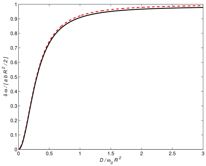
Figure 4: $2\delta\omega/abR^{2}$ versus $y={D}/{R^{2}\omega_{o}}$, equation (73). Black first term, red sum of first 4 terms

References

• (1) Eugene D. Commins, Am. J. Phys. 59, 1077 (1991).
• (2) J.M. Pendlebury et al., Phys Rev. A to be published (2004).
• (3) N.F. Ramsey, Phys. Rev. 100, 1191 (1955).
• (4) D.D. McGregor, Phys. Rev. A 41, 2631 (1990).
• (5) G.D. Cates, S.R. Schaefer, and W. Happer, Phys. Rev A 37, 2877 (1988).
• (6) G.D. Cates et al., Phys. Rev A 38 (1988).
• (7) S.K. Lamoreaux, Phys. Rev. A 53, R3705 (1996).
• (8) A. Abragam, Principles of Nuclear Magnetism (Clarendon Press, Oxford, 1961).
• (9) R. Golub and S.K Lamoreaux, Physics Reports 237, 1-62 (1994).
• (10) A. Sommerfeld, Partial Differential Equations (New York, Academic Press, 1967).
• (11) This theorem, apparently based on work of DeGennes [12], was first stated by Egelstaff [13], and has been cited by many authors, (e.g. [13,14,15]), with slightly different numerical constants. The most complete proof is given in [15]. The form we have used is appropriate for our  two dimensional problem. In appendix 2 we give a detailed discussion and a new proof of the theorem.
• (12) P.G. DeGennes, Physica 25, 825 (1959)
• (13) Peter A. Egelstaff, An introduction to the liquid state, Academic Press, 1967
• (14) Stephen W. Lovesey, Theory of neutron scattering from condensed matter, vol. 1 (Oxford : Clarendon Press ; New York : Oxford University Press, 1984).
• (15) G.L. Squires, Introduction to the theory of Thermal Neutron Scattering. Cambridge University Press, (1978)
• (16) Philip M. Morse and Herman Feshbach, Methods of Theoretical Physics (McGraw-Hill, New York, 1953), (Chapter 7).
• (17) S.K. Lamoreaux et al., Europhys. Lett. 58, 718 (2002).
• (18) Peter A. Egelstaff, Inelastic scattering of neutrons in solids and liquids, IAEA, Vienna, 1961, page 25. See also P.A. Egelstaff, S.J. Cocking and R. Royston ibid, page 309.
• (19) Jean P. Boon and Sidney Yip, Molecular Hydrodynamics, McGraw Hill, 1981 (Dover edition, 1991)
• (20) K. Carneiro, Phys. Rev A14, 517 (1976).
X