Radiation Damage of Polypropylene Fiber Targets in Storage Rings

Abstract

Thin polypropylene (${\rm CH}_{2}$) fibers have been used for internal experiments in storage rings as an option for hydrogen targets. The change of the hydrogen content due to the radiation dose applied by the circulating proton beam has been investigated in the range $1\cdot 10^{6}$ to $2\cdot 10^{8}$ Gy at beam momenta of 1.5 to 3 GeV/c by comparing the elastic pp-scattering yield to that from inelastic p-carbon reactions. It is found that the loss of hydrogen as a function of applied dose receives contributions from a fast and a slow component.

1 Introduction

Polymers are widely used as target materials in nuclear- and particle-physics experiment, since they provide an effective proton target due to the large hydrogen content. As an example polypropylene fiber targets of $4\times 5$ $\mu$m² cross section have been used for the EDDA-experiment [1] at COSY [2] to measure precise excitation functions of the unpolarized differential cross section at beam energies from 0.5 to 2.5 GeV.

For polypropylene the H:C ratio should be 2:1, however, upon irradiation of the target this ratio is going to decrease due to so-called cross-linking [3, 4] of the ${\rm CH}_{2}$-chains, a process in which H₂-molecules are released when C–C bonds replace two C-H bonds. Losses of hydrogen or carbon due to nuclear reactions of the beam protons are negligible in comparison.

In an internal target experiment both the beam position and width change during acceleration [5, 6], such that an experiment will sample different areas of the target at different beam-momenta [6]. As the applied dose will also vary with beam position the effective thickness of the hydrogen target will become a function of beam momentum, as soon as the area of the beam-target overlap changes.

In this paper we investigate the dependence of the hydrogen loss on the applied dose by irradiating a ${\rm CH}_{2}$ fiber target under very controlled conditions. The number density, i.e. hydrogen atoms per volume, for polypropylene is given by (see Tab. 1 for our notation)

$$n_{\rm H,0}=\frac{2\,\varrho_{\rm CH_{2}}\,N_{A}}{M_{\rm CH_{2}}}.$$ (1)

which will change when the target has been irradiated with some dose $D$. If we introduce a normalized hydrogen density $\varrho_{N}$, it will be a function of the applied dose, and thus of position $x$ along the fiber and time:

$$\varrho_{N}(x,t)=\varrho_{N}(D(x,t))=\frac{n_{\rm H}(D(x,t))}{n_{\rm H,0}}.$$ (2)

The aim of this paper is to determine $\varrho_{N}(D)$. We used a stored proton beam at the COSY-accelerator at Jülich on a ${\rm CH}_{2}$-fiber target, and recorded the ratio of the pp-elastic scattering yield to that of proton-carbon inelastic scattering as a function of time. This ratio directly determines dose related changes in $\varrho_{N}$. The scattering yield of elastic pp-scattering allows a precise determination of the luminosity and the COSY beam parameters, like width and position. Using this information the applied dose $D(x,t)$ can be calculated with accuracy.

$x$ :	coordinate along the fiber target.
$y$ :	coordinate orthogonal to the beam and fiber.
$z$ :	coordinate along the COSY-beam axis
$t_{c}$ :	time during COSY’s machine cycle
$N_{c}$ :	number of COSY cycles measured
$dy,dz$ :	thickness of the fiber in the vertical and longitudinal directions
$A=dy\cdot dz=20\ \mu{\rm m}^{2}$ :	cross section of the fiber
$N_{A}$ :	Avogadros number
$\varrho_{\rm CH_{2}}=0.905\frac{\rm g}{\rm cm^{3}}$ :	density of polypropylene
$M_{\rm CH_{2}}=14\frac{\rm g}{\rm mol}$ :	molar mass of ${\rm CH}_{2}$
$\sigma_{x}(t_{c}),\sigma_{y}(t_{c})$ :	horizontal and vertical beam width (standard deviation)
$x_{b}(t_{c})$ :	horizontal beam position (centroid)
$I$ :	beam current.
$e_{0}$ :	elementary charge.
p :	beam momentum.
$\frac{{\rm d}m}{{\rm d}l}$ :	mass per unit length of the fiber.
$\left.\frac{{\rm d}E}{{\rm d}z}\right|_{T<T_{\rm cut}}$(p) :	restricted energy loss [7] of protons in polypropylene.
$n_{\rm H}$ :	number density of hydrogen atoms in polypropylene.
$n_{\rm H,0}$ :	number density of hydrogen atoms in undamaged polypropylene $n_{\rm H,0}=2N_{A}\varrho_{\rm CH_{2}}/M_{\rm CH_{2}}$.
$\varrho_{N}=n_{\rm H}/n_{\rm H,0}$ :	density of hydrogen atoms normalized to the value of undamaged polypropylene.
$D(x,t)$ :	dose distribution along the fiber target as a function of time.

Table 1: Notation and variables used throughout this paper.

In section 2 the EDDA experiment is described, the formalism used to analyze the data in order to extract the hydrogen density as a function of dose is the topic of section 3. The results are presented and discussed in section 4.

2 Experiment

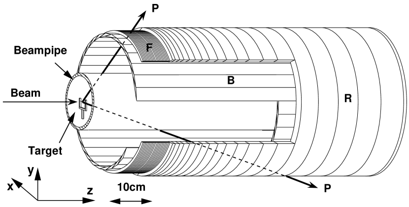
Figure 1: The EDDA detector (not to scale): target: fiber (${\rm CH}_{2}$ or C); B: scintillator bars; R: scintillator semi-rings; F: semi-rings made of scintillating fibers.

The EDDA experiment [1, 8, 9] has been designed to measure differential cross sections, analyzing powers and spin correlation parameters of elastic proton-proton scattering over a wide energy (0.5-2.5 GeV) and angular (30^∘- 90^∘ in the c.m.) range. A schematic view of the EDDA detector is shown in Fig. 1. It is a cylindrical scintillator hodoscope optimized to efficiently detect two protons from elastic pp scattering in coincidence. Elastic events are identified by coplanarity with the beam and the kinematic correlation of the scattering angles $\tan\theta_{\rm lab,1}\cdot\tan\theta_{\rm lab,2}=\gamma_{\rm c.m.}^{-2}$, where $\gamma_{\rm c.m.}$ is the Lorentz-parameter of the c.m. system in the lab.

For this study scattering data acquired at fixed energies of 3.0 and 1.455 GeV/c with ${\rm CH}_{2}$ and carbon targets, detected primarily for the purpose of detector calibration, have been used. The fibers are suspended to a 30 mm wide fork and coated with 20 $\mu$g/cm² aluminum to avoid charge buildup on the target. The targets are mounted on a linear actuator and can be moved in and out of the beam. The experiment is conducted during many COSY machine cycles: after beam injection into COSY, the beam is accelerated to the desired beam momentum, then the fiber target is moved in and data is taken. Since beam-lifetimes are of the order of a few seconds the target is moved out after 5 to 10 seconds, and COSY is reset to be prepared for the next cycle.

3 Analysis

For the analysis data has to be sorted as a function of the time $t_{c}$ an event occurred within a cycle, i.e. $t_{c}$ is the time elapsed since moving in the target. Due to beam-heating by the target, the width and eventually the position of the COSY beam, and thus the dose distribution, change with $t_{c}$, however, they are stable from one cycle to another. The target was first irradiated for about 5 h at a beam momentum of 3.0 GeV/c and then for another 5 h at 1.455 GeV/c. The complete data set was subdivided in small sets comprising data of typically 70 machine cycles, corresponding to roughly 15 minutes of data taking.

3.1 Overview

The dose per time interval ${\rm d}t_{c}$ acquired over $N_{c}$ machine cycles is a function of the horizontal position $x$ along the fiber and the time $t_{c}$ during COSY’s machine cycle. It is given by the product of the average energy deposit $\Delta E$ per particle and the number of particles hitting the target per unit length of the fiber divided by its mass per unit length:

$$\frac{{\rm d}D}{{\rm d}t_{c}}(x,t_{c})=\overbrace{\left.\frac{{\rm d}E}{{\rm d}z}\right|_{T<T_{\rm cut}}\!\!\!\!\!\!\!\!\!\!\!\!\!\!\!(p)\ dz}^{\Delta E}\ (\displaystyle\sum_{c=1}^{N_{c}}\overbrace{\frac{I(t_{c},c)\,dy}{e_{0}\,\sqrt{2\pi}\,\sigma_{y}}}^{\d{N_{p}}/{\rm d}t_{c}})\ \overbrace{\frac{1}{\sqrt{2\pi}\,\sigma_{x}}e^{-\frac{(x-x_{b})^{2}}{2\sigma_{x}^{2}}}}^{\rm beam\ profile}\ \overbrace{\frac{1}{\varrho_{\rm CH_{2}}\,A}}^{{\rm d}l/{\rm d}m}.$$ (3)

Of these quantities the beam current $I$ and the vertical beam width $\sigma_{y}$ are hard to measure precisely. However, the luminosity – with respect to hydrogen – along the target contains the same parameters

$$\frac{{\rm d}L_{H}}{{\rm d}x}(x,t_{c})=\sum_{c=1}^{N_{c}}\overbrace{\frac{I(t_{c},c)\,dy}{e_{0}\,\sqrt{2\pi}\,\sigma_{y}}}^{\d{N_{p}}/{\rm d}t_{c}}\ \overbrace{n_{\rm H,0}\,\varrho_{N}(x,t_{c},c)\,dz}^{\rm target\ area\ density}\ \overbrace{\frac{1}{\sqrt{2\pi}\,\sigma_{x}}e^{-\frac{(x-x_{b})^{2}}{2\sigma_{x}^{2}}}}^{\rm beam\ profile}.$$ (4)

In the experiment we access the luminosity by detecting elastic scattering events $N_{\rm pp}$ for $N_{c}$ machine cycles as a function of $t_{c}$. Due to the finite resolution in determining the x-coordinate of the scattering vertex only the total luminosity, e.g. integrated over $x$, is available:

$$L_{H}(t_{c},N_{c})=\displaystyle\int_{-\infty}^{\infty}{\rm d}x\frac{{\rm d}L_{H}}{{\rm d}x}(x,t_{c})=\displaystyle\frac{N_{\rm pp}(t_{c})}{\sigma_{\rm pp}\,[1-\tau(t_{c})]\,\epsilon}.$$ (5)

Here, $\sigma_{\rm pp}$ is the differential cross section integrated over the accepted solid angle, $\tau$ the deadtime of the data acquisition system and $\epsilon$ the detection efficiency, i.e. mainly a correction for losses of elastic events due to secondary reactions in the detector.

Note, that the target density itself changes with the dose applied and will be both position and time dependent, so that the integration of Eq. (4) cannot be carried out directly. However, we can adopt an iterative approach and set $\varrho_{N}$ to unity as a first approximation, which will overestimate the luminosity. The true luminosity will be smaller by the weighted average over $x$ of the normalized hydrogen density, introduced via

$$\overline{\varrho_{N}}(t_{c})=\frac{\displaystyle\sum_{c=1}^{N_{c}}I(t_{c},c)\int_{-\infty}^{\infty}{\rm d}x\varrho_{N}(x,t_{c},c)\ \frac{1}{\sqrt{2\pi}\,\sigma_{x}}e^{-\frac{(x-x_{b})^{2}}{2\sigma_{x}^{2}}}}{\displaystyle\sum_{c=1}^{N_{c}}I(t_{c},c)},$$ (6)

a correction, we will have to determine using the relation $\varrho_{N}(D)$ to be established in Sec. 4, where in turn $D$ is a function of $x$, $t_{c}$ and the individual cycle. Again in a first approximation $\overline{\varrho_{N}}$ will be set to one, and recalculated in the following iterations. Now we may write Eq. (5) by inserting Eq. (4) as

$$L_{H}(t_{c},N_{c})=\overline{\varrho_{N}}(t_{c})\sum_{c=1}^{N_{c}}\frac{I(t_{c},c)}{e_{0}}\cdot\frac{dy\,dz\,n_{\rm H,0}}{\sqrt{2\pi}\,\sigma_{y}}$$ (7)

and thus

$$\frac{dy\,dz\,\sum_{c=1}^{N_{c}}I(t_{c},c)}{\sqrt{2\pi}\,\sigma_{y}\,e_{0}}=\frac{L_{H}(t_{c},N_{c})}{n_{\rm H,0}\,\overline{\varrho_{N}}(t_{c})}=\frac{M_{\rm CH_{2}}}{2\,N_{A}\,\varrho_{\rm CH_{2}}}\cdot\frac{L_{H}(t_{c},N_{c})}{\overline{\varrho_{N}}(t_{c})}.$$ (8)

Note, that this derivation holds, even when the vertical target position $y_{t}$ is not centered at the vertical location of the beam $y_{b}$, since the additional factor $\exp(-[y_{t}-y_{b}]^{2}/2\sigma_{y}^{2})$ in Eqs. (3) and (4) cancels.

Insertion in Eq. (3) finally replaces $I$ and $\sigma_{y}$ by experimentally accessible quantities

$$\frac{{\rm d}D}{{\rm d}t_{c}}(x,t_{c})=\overbrace{\left.\frac{{\rm d}E}{{\rm d}z}\right|_{T<T_{\rm cut}}\!\!\!\!\!\!\!\!\!\!\!\!\!\!\!(p)\ \ \ \ \frac{M_{\rm CH_{2}}}{2\,N_{A}\,\varrho_{\rm CH_{2}}^{2}\,A}}^{k(p)}\cdot\frac{L_{H}(t_{c},N_{c})}{\overline{\varrho_{N}}(t_{c})}\cdot\frac{1}{\sqrt{2\pi}\,\sigma_{x}}e^{-\frac{(x-x_{b})^{2}}{2\sigma_{x}^{2}}}.$$ (9)

This must be integrated over $t_{c}$ to obtain the dose profile $D(x)$ along the beam acquired during $N_{c}$ machine cycles.

The restricted energy loss $\left.\frac{{\rm d}E}{{\rm d}z}\right|_{T<T_{\rm cut}}$ [7] is the energy loss due to ionization, corrected for the energy carried away by $\delta$ electrons with energies $T>T_{\rm cut}$ escaping from the target. By requiring the practical range of electrons [10] to be half of the ${\rm CH}_{2}$-target thickness ($\approx$ 0.2 mg/cm²) and taking the thin aluminum-coating ($\approx$ 20 $\mu$g/cm²) into account we deduce a value of 9 keV for $T_{\rm cut}$. Using ionization-loss parameters of [11] we obtain numerical values for the constant $k(p)$ of 190.9 (155.0) ${\rm Gy\,mm\,mb}$ at 1.455 (3.0) GeV/c.

To summarize, we need to deduce the integrated luminosity $L_{H}$, the beam position and width from the scattering data in order to obtain the dose profile along the fiber. As pointed out earlier, Eqs. (6) and (9) can only be solved iteratively. One starts by assuming $\overline{\varrho_{N}}$($t_{c}$) being unity, and then arrives at a dose which will be underestimated. From the measured change in hydrogen density as a function of the dose (cf. Eq. (12)) $\overline{\varrho_{N}}$($t_{c}$) is recalculated and a better estimate of the dose is found. After at most two iteration self-consistency is reached.

3.2 Luminosity

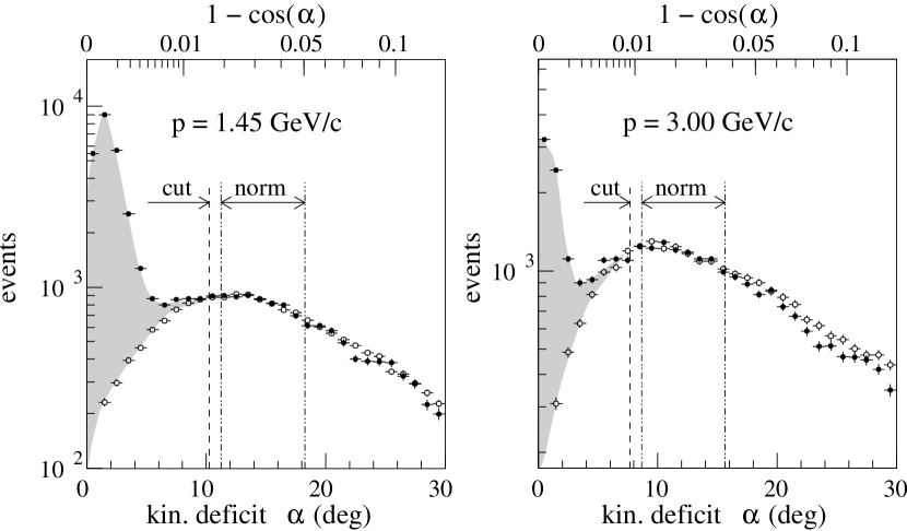
Figure 2: Distribution of the kinematic deficit $\alpha$ for data taken with a ${\rm CH}_{2}$(solid) and C-targets (open symbols, normalized to the ${\rm CH}_{2}$-data). The upper limit in $\alpha$ used to select elastic scattering events (cut) is indicated as well as the range (norm) used to determine the relative luminosity with respect to scattering of carbon for the two targets.

For the luminosity determination, using Eq. (5), we need the total number of elastic scattering events. These are identified by looking at the so-called “kinematic deficit”, the angle $\alpha$ of the deviation from a perfect back-to-back correlation of the two detected prongs in the c.m., when transformed assuming an angle-energy correlation as for pp elastic scattering. As evinced in Fig. 2, pp elastic scattering events stand out at very small $\alpha$ with very little background from proton-carbon scattering. We use a cut at 10.2^∘(7.7^∘) at 1.455 (3.0) GeV/c for accepted events. The geometric acceptance of the EDDA-detector is taken into account by using only events with polar angles between 36^∘(38^∘) and 90^∘ in the c.m. for the forward proton. In addition, events with an azimuthal angle within $\pm 15$^∘ around 90^∘ or 270^∘ are excluded, where the angle measurement of $\theta_{\rm c.m.}$  has reduced accuracy owing to the inhomogeneous light-collection close to the attached light-guides. The contribution from proton-carbon scattering is removed by subtracting the yield from scattering of a carbon target using the same cuts and normalized to the same number of counts in the tails of the $\alpha$-distribution as indicated in Fig. 2.

The pp-elastic scattering cross section, cf. Eq. (5), is obtained by numerical integration of the differential cross section as given by the solution FA00 [12] of the VPI/GW phase shift analysis.

Further corrections are applied to account for losses due to secondary reactions of the ejectiles in the detector (5%) and for the deadtime of the data-acquisition event-builder, deduced from the ratio of triggers read out by the DAQ-system to the total number of triggers, which is accomplished by 20 MHz scalers, read out every 2.5 ms. Details are given in [1, 5]. The deadtime ranges from 90% at the beginning to 10% at the end of the cycle. The resulting luminosity is shown at the top of Fig. 3.

3.3 Beam Parameters

Figure 3: Luminosity (top), horizontal beam position (center) and width (bottom) as a function of time during the COSY-cycle (here $t_{c}$=0 has been set to the time the target is moved in) for beam momenta of 1.455 and 3.3 GeV/c.

The beam position and width can be inferred from pp elastic scattering data as well, by exploiting the coplanarity of the two protons with the beam. The beam position and width as well as the azimuthal angular resolution are obtained from a nonlinear ${\chi^{2}}$-fit of data with different values of the azimuthal angle $\phi$. The procedure is described in detail elsewhere [6], the results for the two beam-momenta are displayed in Fig. 3.

The increase of the beam-width or emittance due to the heating of the stored beam is clearly visible. At 1.455 GeV/c the movement of the beam at the end of the cycle is due to the beginning deceleration, whereas the jump in position at mid-cycle of the 3.0 GeV/c data is caused by exciting horizontal steerer used to cross-check the vertex-reconstruction.

3.4 Hydrogen Density

The relative change of the hydrogen density in the target is proportional to the ratio of $N_{\rm pp}$, i.e. the shaded area in Fig. 2, and the number of proton-carbon scattering events $N_{\rm pC}$. For the latter we use the number of events in the range $11^{\circ}<\alpha<25^{\circ}$ of Fig. 2, mainly populated by quasi-free proton-proton scattering. To this end the normalized hydrogen density is given by

$$\varrho_{N}=f(p)\frac{N_{\rm pp}}{N_{\rm pC}}$$ (10)

with a momentum-dependent proportionality constant $f(p)$ which needs to be determined from the data.

4 Results and Discussion

The data has been subdivided into 43 subsets, 21 at 3.0 GeV/c and 22 at 1.455 GeV/c, and a value for $\varrho_{N}/f(p)$ has been deduced viz Eq. (10). This needs to be related to the dose acquired prior and during data taking of this subset. Since $\varrho_{N}$ is averaged over the horizontal beam profile, we relate it to the corresponding average dose

$$\bar{D}=\frac{\displaystyle\int{\rm d}t_{c}\ N_{\rm pp}(t_{c})\ \int{\rm d}x\ D(x,t_{c})\ \frac{1}{\sqrt{2\pi}\,\sigma_{x}}e^{-\frac{(x-x_{b})^{2}}{2\sigma_{x}^{2}}}}{\displaystyle\int{\rm d}t_{c}\ N_{\rm pp}(t_{c})},$$ (11)

where we implicitly assume, that an appropriate summation over the number of cycles has been done. For simplicity, we will denote this dose by $D$ subsequently.

For the functional dependence of $\varrho_{N}(D)$ we tried a simple ansatz of a linear or exponential decrease, which turned out to be insufficient to describe the data. We obtained a successful fit with the following expression:

$$\varrho_{N}(D)=\frac{n_{\rm H}}{n_{\rm H,0}}(D)=a\exp(-\lambda_{1}D)+(1-a)\exp(-\lambda_{2}D),$$ (12)

using a total of five fit parameters $a$, $\lambda_{1,2}$, $f$(1.455 GeV/c), and $f$(3.0 GeV/c). The result is shown in Fig. 4.

When iterating Eqs. (6) and (9), the average hydrogen density for a sample is given by

$$\overline{\varrho_{N}}=\displaystyle\frac{1}{\Delta D}\int_{D_{0}}^{D_{0}+\Delta D}{\rm d}D\,\varrho_{N}(D),$$ (13)

where $D_{0}$ and $\Delta D$ are the dose applied prior and during the measurement of the sample. After two iterations self-consistency is reached and we obtain the fit values

$$\begin{array}[]{r@{\ =\ (}l@{\ \pm\ }l@{)\ }l}\lambda_{1}&4.4&1.3&\cdot 10^{-8}\ {\rm Gy}^{-1}\\ \lambda_{2}&5.67&0.28&\cdot 10^{-10}\ {\rm Gy}^{-1}\\ a&5.8&0.7&\%\\ \end{array}$$ (14)

where errors are purely statistical. The systematic error is dominated by uncertainties in the area $A$ of the target cross-section (10%) and the restricted energy loss (4%), where the exact value depends on the choice of $T_{\rm cut}$. This leads to a 11% scale uncertainty of the dose and consequently of $\lambda_{1}$ and $\lambda_{2}$.

The normalized hydrogen density $\varrho_{N}$ of Eq. (10), determined from the experiment, is in fact the average over the length of the fiber. It receives contributions from regions with quite different accumulated dose, which are weighted with the beam intensity distribution and averaged over the machine cycle. It can be shown, however, that the correct functional dependence is obtained when $\varrho_{N}$(D) is a linear function. The systematic effect caused by the deviation from linearity in Eq. (12) was checked numerically and is always smaller than 0.25% in $\varrho_{N}$, and can therefore be neglected.

Figure 4: Normalized hydrogen density as a function of applied dose. The result of the fit is shown as the solid line. The dashed line shows the contribution of the slow component only. Note, that the first data point at 1.455 GeV/c corresponds to a lower dose than the last point at 3.0 GeV/c, since the beam is slightly displaced, such that a region of lower accumulated dose is probed.

Figure 5: G-value for cross-linking as a function of the accumulated dose.

Assuming that the loss of hydrogen is entirely due to cross-linking, our results may be compared to the so-called $G$-value [4] found in the literature. It describes the number of cross links $\delta N_{X}$ per $\delta E=100$ eV energy deposited in the polymer. Since per cross-link two hydrogen atoms are lost, the change of hydrogen density for a sample of volume $V$ and mass $m$ is given by

$$-\frac{{\rm d}\varrho_{N}}{{\rm d}D}\approx\frac{1}{n_{\rm H,0}}\cdot\frac{2\delta N_{X}}{V}\cdot\frac{m}{\delta E}=\frac{\varrho_{\rm CH_{2}}}{n_{\rm H,0}}\cdot\frac{2G}{\delta E}=\frac{M_{\rm CH_{2}}}{N_{A}}\cdot\frac{G}{\delta E}.$$ (15)

Solving for G using Eq. (12) yields

$$G=\frac{\delta E\ N_{A}}{M_{\rm CH_{2}}}\left[a\lambda_{1}\exp(-\lambda_{1}D)+\lambda_{2}(1-a)\exp(-\lambda_{2}D)\right]$$ (16)

which is displayed in Fig. 5. It nicely agrees with the range of G-values 0.3 to 1.1 [13] and $0.6\pm 0.1$[14] found in the literature. However, we find that the G-value is not a constant but depends on the irradiation-history of the target. The data of [14, 15], obtained by a similar measurement with 14.5 MeV protons on 14 $\mu$m thick polypropylene fibers but with much lower statistical precision, are in agreement with this finding.

5 Summary

Thin ${\rm CH}_{2}$-fiber targets have been irradiated by 1.455 and 3.0 GeV/c protons at an internal target station of the COSY accelerator. The applied dose distribution was deduced from the elastic scattering rate measured continuously during irradiation. The hydrogen density was monitored by observing the relative yield of proton-proton elastic scattering with respect to proton-carbon inelastic reactions. The hydrogen loss as a function of dose can be described by a fast component responsible for at most 6% of the total loss, and a slow component corresponding to G-value of about 0.35. The loss rate, attributed to cross-linking of the chains within the polymer, is in-line with published values. Detailed knowledge of the observed strong dependence on the accumulated dose of a polypropylene-target will be important for experiments aiming at absolute cross-sections, where the hydrogen-density needs to be known accurately as a function of time as well as vertex position that may vary considerably during acceleration [5].

References

- [1] D. Albers, et al., Phys. Rev. Lett. 78 (1997) 1652–1655.
- [2] R. Maier, Nucl. Instr. and Meth. A390 (1997) 1.
- [3] A. Charlesby, Nucleonics 14 (1956) 82.
- [4] R. Bradley, Radiation Technology Handbook, Marcel Dekker Inc., New York, 1984.
- [5] D. Albers, et al., nucl-ex/0403045, submitted to Eur. Phys. J. A.
- [6] H. Rohdjeß, et al., nucl-ex/0403043, submitted to Nucl. Instr. and Meth. A
- [7] Particle-Data-Group, K. Hagiwara et al., Review of particle physics, Phys. Rev. D 66 (2002) 010001, see also http://pdg.lbl.gov.
- [8] M. Altmeier, et al., Phys. Rev. Lett. 85 (2000) 1819.
- [9] F. Bauer, et al., Phys. Rev. Lett. 90 (2003) 142301.
- [10] J. A. Gledhill, J. Phys. A 6 (1973) 1420.
- [11] P. J. F. Janni, At. Data and Nucl. Data Tables 27 (1982) 147–529.
- [12] R. A. Arndt, I. I. Strakovsky, R. L. Workman, Phys. Rev. C 62 (2000) 34005.
- [13] R. J. Wood, A. K. Pikaev, Applied Radiation Chemistry: Radiation Processing, John Wiley and Sons, Inc., New York, 1994.
- [14] F. Mosel, Ph.D. Thesis, University of Bonn, Germany (1994)
- [15] F. Mosel, Diploma Thesis, University of Bonn, Germany (1991)