Determining Beam Parameters in a Storage Ring with a Cylindrical Hodoscope using Elastic Proton-Proton Scattering

Abstract

The EDDA-Detector at the Cooler-Synchrotron COSY/Jülich has been operated with an internal ${\rm CH}_{2}$ fiber target to measure proton-proton elastic scattering differential cross sections. For the data analysis knowledge of beam parameters, like position, width and angle, are indispensable. We have developed a method to obtain these values with high precision from the azimuthal and polar angles of the ejectiles only, by exploiting the coplanarity of the two final state protons with the beam and the kinematic correlation. The formalism is described and results for beam parameters obtained during beam acceleration are given.

1 Introduction

In nuclear and particle physics experiment knowledge of the distribution of scattering vertices is a crucial ingredient of data analysis. In most cases experiments are designed to yield enough position information to trace detected particles back to the origin. However, even with a much simpler detector, events with particularly simple topologies like elastic scattering may allow to extract the vertex distribution with much lesser experimental information.

The EDDA experiment [1, 2] at the COSY accelerator [3] in Jülich is dedicated to the measurement of pp elastic scattering over a wide energy (0.5-2.5 GeV) and angular range (30^∘ to 90^∘ in the c.m.). The experimental program includes measurements of the unpolarized differential cross-section [1, 2], analyzing power [4] and spin-correlation parameter [5]. Data taking for unpolarized cross section was done only with the outer part of the EDDA-detector, shown in Fig. 1, detecting in coincidence a single point of incidence for each of the two protons, originating from elastic scattering of the internal proton beam from $5\times 4\ \mu$m² thin ${\rm CH}_{2}$-fiber targets. However, for the reconstruction of scattering angles, detector calibration, and luminosity determination detailed knowledge of the beam-target overlap is important. Since measurements were taken during acceleration of the COSY-beam, such that beam position and width are a function of beam-momentum, it was mandatory, that these quantities can be determined from the scattering data itself.

Two-body kinematics require the two protons to be coplanar with the beam. Thus deviations from coplanarity of proton-proton scattering events with the detector symmetry axis bears information on the position and angle of the COSY beam axis with respect to the detector. Along these lines we developed a method to extract information on beam and target parameters like width, position and angle from a single-layered detector described in this paper. In sections 2 and 3 we will give a brief description of the experiment and the selection of scattering data. Section 4 will explain the formalism and in section 5 some examples for the application of this method will be discussed.

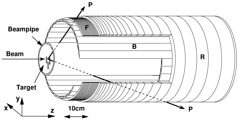
Figure 1: Schematic drawing of the EDDA detector

2 Experiment

The EDDA Detector (cf. Fig. 1) measures the point of interception of the two final-state particles of proton-proton scattering events with a cylindrical symmetric scintillator array around the COSY beam pipe. It consists of a layer of 32 overlapping scintillator bars (B) of triangular cross section detecting the azimuthal angle $\phi$ and a layer of 2$\times$29 semirings, made either from bulk scintillator (R) or scintillating fibers (F), detecting the position $z$ of incidence along the symmetry axis of the detector and bears information on the polar angle $\theta_{\rm lab}$. The angular resolution is improved by about a factor of five with respect to the granularity by comparing off-line the light output of two adjacent detector elements [6].

Thin ${\rm CH}_{2}$- or carbon-fibers, stretched horizontally on a 30 mm wide fork, are used as targets. They can be moved vertically in and out of the beam by a magnetic drive. Beam lifetimes of 3 to 10 s, depending on beam energy, have been achieved. Data is taken during and/or after acceleration of the COSY-beam and accumulated over many machine cycles to obtain statistical precision. Hits in opposing bars serve as a coplanarity trigger. In addition, elastic scattering kinematics

$$\cot\theta_{\rm lab,1}\cdot\cot\theta_{\rm lab,2}=\frac{z_{1}\cdot z_{2}}{R_{R}^{2}}=\gamma_{\rm c.m.}^{2},$$ (1)

with $\gamma_{\rm c.m.}$ being the Lorentz-factor of the c.m. in the laboratory and $R_{R}$ the radius of the ring-layer, is tested by a coincidence of two semiring with appropriate locations in $z$.

3 Event Selection

Figure 2: Distribution of the kinematic deficit $\alpha$ for scattering events at a beam momentum of 1.455 GeV/c. The upper limit for accepted elastic scattering events is shown as the vertical line.

Coplanarity and the kinematic correlation (cf. Eq. (1)) can be tested with refined precision offline. Then two prongs detected in coincidence are transformed to the c.m. system, with the hypothesis of being elastically scattered protons. For pp elastic scattering events these prongs should be back-to-back in the c.m. system, and the angular deviation $\alpha$ from this signature, the so-called kinematic deficit, should be small. A typical distribution is shown in Fig. 2. The apparent contribution from the carbon contents of the target is measured separately using pure C-targets and subtracted statistically. To this end two data sets taken with a ${\rm CH}_{2}$- and a C-target under the same experimental conditions are subject to an identical offline analysis. The relative normalization of the two samples with respect to proton-carbon reactions is derived from the counts in the range 10^∘ to 15^∘in $\alpha$ (cf. Fig. 2), mainly populated by quasi-free scattering on protons bound in carbon. This normalization factor is used to subtract the contribution from pC scattering in all acquired experimental spectra, so that a clean pp elastic scattering sample is available. Monte-Carlo simulations showed this procedure also takes care of the small contribution from inelastic pp-reactions in first order. Details of the event reconstruction are described elsewhere [1, 2].

4 Formalism

In this section we will use a coordinate system ($x,y,z$) attached to the EDDA detector as shown in Fig. 1, with the $z$-axis being the symmetry axis of the detector pointing downstream from the target (at $z=0$) with respect to the COSY-beam, the $y$-axis pointing upward in the lab, and the $x$-axis pointing outboard of the COSY-ring. If not stated otherwise all quantities will be given in this detector coordinate system. Widths given as standard deviation are denoted by $\sigma$, while $\delta$ signifies FWHM (full width at half maximum)

The distribution of scattering vertices must be along the fiber target, which have negligible (4-5 $\mu$m) spatial extension in the $y$- and $z$-directions. The longitudinal target position along $z$ can be determined from scattering data using Eq. (1) and defines the zero of the coordinate system in this direction. Finally, the parameters yet to be determined are

	$y_{b}$	fiber target position in $y$ at $z$=0.
$x_{b}$	beam position in $x$ at $z$=0 and $y_{b}$.
$x^{\prime}_{b}$	horizontal beam angle (d$x$/d$s$) at $z$=0.
$y^{\prime}_{b}$	vertical beam angle (d$y$/d$s$) at $z$=0.
$\delta x_{b,FWHM}$	size of the beam in $x$ at $z$=0 and $y_{b}$.
$\delta\phi$	detector resolution in the azimuthal angles $\phi_{1}$ and $\phi_{2}$.

For simplicity the formalism will first be described for a beam parallel to the detector symmetry axis, i.e. $x^{\prime}_{b}$= $y^{\prime}_{b}$= 0. The generalization to tilted beams will be the topic of Section 4.2

4.1 Beam Parallel to the Detector Axis

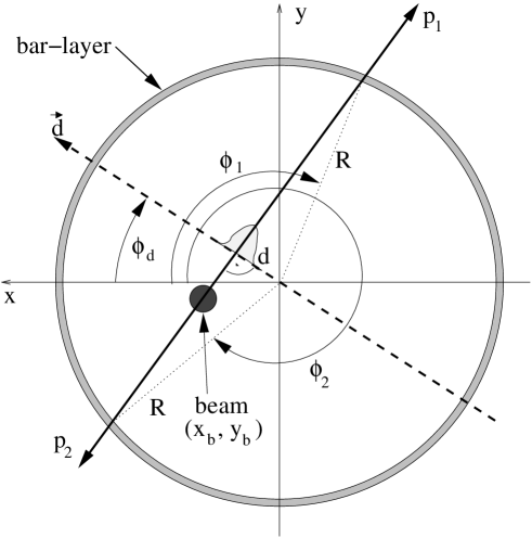
Figure 3: Geometry for a beam parallel to the detector symmetry axis $z$ as explained in the text.

Consider a beam displaced by ($x_{b}$,$y_{b}$) in the $x$,$y$-plane from the detector symmetry axis. In a projection on the $x$,$y$-plane of an elastic scattering event (prongs $p_{1}$ and $p_{2}$ in Fig. 3) a beam displacement leads to a deviation from coplanarity when the vertex is assumed to be at ($x$,$y$)=(0,0) (dotted lines).

The EDDA detector measures the point of interception of these two prongs with the bar layer at a mean radius of $R=164$ mm. Connecting these two points by a straight line its distance $d$ to the origin of the coordinate system is a function of the beam position. If we now define an axis $\vec{d}$ perpendicular to this line (fat dashed line in Fig. 3) we can calculate the angle $\phi_{d}$ of the $\vec{d}$ axis to the $x$-axis

$$\phi_{d}=\frac{\phi_{1}+\phi_{2}}{2}$$ (2)

and the position $d$ along this axis:

$$d=-R\cos\frac{\phi_{1}-\phi_{2}}{2}$$ (3)

The orientation of the $\vec{d}$ axis has been chosen to point to the “left”, to the effect that $\phi_{d}\in[-\pi/2,\pi/2]$ must be forced by adding or subtracting $\pi$ from the expression given in Eq. (2) (For the example of Fig. 3 $\pi$ must be subtracted). The negative sign in Eq. (3) is due to this choice. Eqs. (2) and (3) are an eventwise transformation from the observables ($\phi_{1}$,$\phi_{2}$) to ($d$,$\phi_{d}$).

The connection between $d$ and the beam position is evident. Using basic trigonometric relations (for a derivation see Appendix A) – or by a simple geometric derivation using Fig. 3 – one obtains:

$$d=x_{b}\cos\phi_{d}+y_{b}\sin\phi_{d}$$ (4)

Now, the idea is to consider the $d$-distribution of events with different $\phi_{d}$ in order to deduce $x_{b}$ and $y_{b}$.

4.1.1 Experimental Input and Analysis

Figure 4: (a) Variation of the $d$-distribution for different bins in $\phi_{d}$. The fit (solid Gaussian) to the data (crosses) yields a beam displacement of $x_{b}=-2.51$ mm, $y_{b}=-0.41$ mm. The mean value is shown as the solid vertical curve, for the dashed curve $y_{b}$ was fixed to zero. (b) Variation of the $d$-distribution at $\phi_{d}=15\pm 5^{\circ}$ with $z_{1}+z_{2}$ and the result of the fit (solid line) yielding $x^{\prime}_{b}~{}\approx 5$ mrad. The dashed line shows the fit at 825 mm for comparison.

For each event $\phi_{d}$ and $d$ are calculated. The events are sorted into spectra vs. $d$ for different ranges in $\phi_{d}$. Events with $|\phi_{d}|<10^{\circ}$ are discarded, since here the readout of the semirings causes trigger inefficiencies. A $d$-distribution is accumulated for 16 $\phi_{d}$-intervals from -90^∘ to -10^∘ and 10^∘ to 90^∘, each 5^∘ wide. These 16 spectra, an example is shown in Fig. 4 (a), are the input to the analysis. For investigation of the time dependence of beam parameters this set of spectra is accumulated for small time intervals, usually 25, 50 or 100 ms wide, separately.

The experimental $d$-distributions can be fitted by a Gaussian

$$n(d)=\frac{N(\phi_{d})}{\sqrt{2\pi}\sigma_{d}}\exp\left(-\frac{(d-\bar{d})^{2}}{\sigma_{d}^{2}}\right)$$ (5)

with two fit parameters $\bar{d}$ and $\sigma_{d}$ bearing the information on the beam. The total number of counts for a given $\phi_{d}$-interval $N(\phi_{d})$ is used for the normalization and kept fixed in the fit.

For a given $\phi_{d}$, the value of $\bar{d}$ is given by Eq. (4) and

$$\sigma_{d}\approx\sqrt{\cos^{2}\phi_{d}\sigma^{2}_{x_{b}}+\frac{R^{2}}{2}\sigma^{2}_{\phi}}$$ (6)

when the vertical size of the target is neglected (cf. Appendix A). Thus all 16 spectra are fitted simultaneously by four fit parameters: $x_{b}$, $y_{b}$, $\sigma^{2}_{x_{b}}$, and $\sigma^{2}_{\phi}$. For the implementation of the fitting procedure the minimizer MIGRAD (variable metric method) of the CERN package MINUIT [7] is used. Typical spectra are shown in Fig. 4 (a) for a 25 ms wide bin in time – corresponding to $\Delta p\approx 29$ MeV/c during acceleration of the COSY beam. Clearly, differences of 0.5 mm in $y_{b}$ can be resolved by the data.

4.1.2 Test of Method

Figure 5: Sketch of the orbit distortion expected for a simultaneous excitation of the horizontal steerer SH5 and SH9. The beam position is measured by EDDA at the indicated position.

Figure 6: Result of the fit for flattop data at 3.4 GeV/c where around 3000-4000 ms a horizontal excursion of the beam was produced by exciting steerer magnets (cf. Fig. 5). The solid line shows the expected shape of the excursion with the amplitude and position in $x_{b}$ adjusted to the data.

Figure 7: Result of the fit for flattop data at 2.25 GeV/c. The fiber target starts to move at 0 ms and reaches the beam position around 250 ms.

As a test of the sensitivity of the method, data at fixed momentum of 3.4 GeV/c was acquired while the beam was moved horizontally across the target by exciting two horizontal steerer dipoles of the COSY-lattice. Between the steerer, separated by a phase advance of about $\pi$, focusing quadrupoles are located, resulting in the geometry of the beam excursion as depicted in Fig. 5. The strength of the magnets (originally at 0%) was ramped within 100 ms to +80%, then, after 10 ms, they were ramped linearly to -100% within 1000 ms and finally –after another 10 ms– brought back to 0% within 100 ms.

The result of the fit (Fig. 6) shows the response of the beam: The beam position $x_{b}$ follows closely the strength of the magnet. The vertical target position $y_{b}$, the beam width $\delta x_{b,FWHM}$, and the angular resolution $\delta\phi$ remain basically unchanged. This proves the sensitivity of this method to the beam position.

Another test is to take data taken at fixed energy and beam position and to observe the increase in beam size due to the emittance growth when the beam is “heated” by the target. The result of the fit is shown in Fig. 7. As expected only the beam size increases with time. All other parameters remain constant. It is interesting to see, that even the overshoot of the target – after is has been moved in vertically during the first 250 ms by a linear actuator and before it settles at the correct height – is resolved. As long as the target moves the vertex is then spread out in $y$ and results in an increased angular width $\delta\phi$ in the fit.

In all figures only statistical errors are given as they are calculated from the error-matrix of the nonlinear $\chi^{2}$-fit. However, systematic errors arise mainly due to strong correlations of fit parameters. In Fig. 7 the anti-correlations of $\delta\phi$ and $\delta x_{b,FWHM}$ introduced by Eq. (6) is clearly visible. Since $R\delta\phi/\sqrt{2}\approx 3.6$ mm the angular resolution in $\phi$ makes it difficult to determine beam sizes smaller than 3 mm accurately. Then, the $\cos^{2}\phi_{d}$ modulation of $\sigma_{d}$ becomes very small and statistical fluctuations start to mislead the fit.

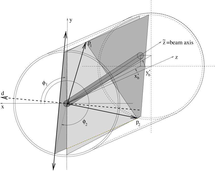
Figure 8: Geometry for a tilted beam (axis $\tilde{z}$ tilted by $x^{\prime}_{b}$, $y^{\prime}_{b}$) as explained in the text.

4.2 Tilted Beam

In the previous section it has been assumed that the beam is parallel to the symmetry axis of the detector. This is not necessarily true. In general, the beam may be tilted with respect to the detector both horizontally and vertically, described by the parameters $x^{\prime}_{b}$  and $y^{\prime}_{b}$. Fig. 8 shows that a tilted, non-displaced beam mocks up a beam displacement in the analysis neglecting $x^{\prime}_{b}$ and $y^{\prime}_{b}$: since only the azimuthal angles are considered, we reconstruct the event in a plane parallel to the detector z-axis, defined by the two points of interception with the EDDA detector (dark shaded plane in Fig. 8). The reaction plane (light plane in Fig. 8) is defined by the same two points but must be coplanar to the beam. Consider a pp-elastic event where the two protons are emitted up-down: if the beam angle $x^{\prime}_{b}$ is positive the two protons tracks will be displaced to the left with respect to their origin. The displacement depends on the distance in $z$ they travel until they hit the EDDA bar layer at radius $R$. As evinced in Fig. 8 the line through the two points of interception projected into the $x$-$y$ plane looks as if the beam were displaced to positive $x$.

In Appendix A it is derived that the measured value of $d$ of a tilted beam is given by:

$$d=(x_{b}+\frac{z_{1}+z_{2}}{2}x^{\prime}_{b})\cos\phi_{d}+(y_{b}+\frac{z_{1}+z_{2}}{2}y^{\prime}_{b})\sin\phi_{d}$$ (7)

and reduces to Eq. (4) for $x^{\prime}_{b}=y^{\prime}_{b}=0$. $z_{1}$ and $z_{2}$ are the $z$-coordinate of the point where the tracks of the proton intercept the EDDA bar layer. Evidently, the parameters $x_{b}$ and $x^{\prime}_{b}$ (as $y_{b}$ and $y^{\prime}_{b}$) are strongly correlated and can only be distinguished by considering events with different $z_{1}+z_{2}$. For pp-elastic scattering the correlation of the two $z$ values as a function of beam kinetic energy $T_{p}$ is given by Eq. (1)

$$z_{1}z_{2}=R^{2}\gamma_{\rm c.m.}^{2}=R^{2}(1+\frac{T_{p}}{2m_{p}})$$ (8)

where $m_{p}$ is the proton mass. The values covered by $z_{1}+z_{2}$ range from $2R\gamma_{\rm c.m.}\approx 400\ldots 500$ mm for symmetric events ($z_{1}=z_{2}$) to $1100$ mm for asymmetric events ($z_{1}=z_{\rm max}=1$ m, see Fig. 1).

Figure 9: Result of the fit for flattop data at 3.4 GeV/c. The solid symbols are the result of the fit when the beam angles $x^{\prime}_{b}$ and $y^{\prime}_{b}$ are included in the fit. The open symbols are the data as in Fig. 6 and the solid lines the expected shape of the excursion.

4.2.1 Experimental Input

For each $\phi_{d}$-bin the data was further subdivided into 14 classes with respect to their $z_{1}+z_{2}$ values, ranging from 400 to 1100 mm, each 50 mm wide. For a given energy only those classes were included in the fit where the kinematics allowed for the respective $z_{1}+z_{2}$ value. Usually 8-13 classes are useful, and for each class 16 $d$ distributions for the different $\phi_{d}$ ranges are sorted. The resulting 128-208 spectra are fitted simultaneously with six parameters $x_{b}$, $y_{b}$, $\sigma_{\phi}$, $\sigma_{x_{b}}$, $x^{\prime}_{b}$, and $y^{\prime}_{b}$. An example of these spectra is shown in Fig. 4 (b) where the shift in $\bar{d}$ with $z_{1}+z_{2}$, containing the information on beam angles is clearly visible through comparison to the result for $z_{1}+z_{2}\approx 825$ mm.

The result of the fit (same data as in Fig. 6) is shown as the solid symbols in Fig. 9. The change in beam angle and the beam position have the same sign as one expects for the geometry shown in Fig. 5. The total change in angle during the bump (4 mrad) and the range of the beam position shift (8 mm) yield a distance of the origin of the beam rotation at -2 m with respect to the target location which agrees rather well with the distance of the steerer magnet SH5 to the fiber target (1.75 m). The fact that the change in $x_{b}$ and $x^{\prime}_{b}$ have the same sign indicates that the method is indeed sensitive to changes in beam angles, since Eq. (7) implies that fluctuations of these parameters due to statistics would be anti-correlated in the fit. Again errors shown are purely statistical, and the observed fluctuations around the expected excursions are now much larger, due to the strong anti-correlation of beam position and angle in the fit. These fluctuations can be only be damped by improving on the statistical precision of the data. Summarizing, possible beam tilts $x^{\prime}_{b}$ and $y^{\prime}_{b}$ should always be taken into account since the results for the beam positions $x_{b}$ and $y_{b}$ depend on $x^{\prime}_{b}$ and $y^{\prime}_{b}$ (compare Figs. 6 and 9).

5 Results and Discussion

Figure 10: Fit parameter as a function of time for data acquired during acceleration and the flattop. Also shown is the momentum of the beam and the signal of a luminosity monitor, the secondary electron monitor (SEM). Solid (open) symbols and solid (dashed) lines show the result of the fit when $x^{\prime}_{b}$ and $y^{\prime}_{b}$ were (were not) included as fit parameters.

The method of reconstructing the first and second moment of the vertex distribution has been applied routinely for data analysis of the EDDA experiment. In Fig. 10 we show an example of a measurement taken during acceleration of the COSY beam and the flattop at 3.3 GeV/c. For comparison both the beam momentum and the response of the secondary electron monitor (SEM) as a measure of the luminosity are shown. In this example the beam position could be held rather stable throughout the ramp, some shifts in the beam angle $x^{\prime}_{b}$ is seen, especially in the transition to the flattop. Most strikingly, the rise in the SEM signal coincides with a dramatic increase in the horizontal beam width. Beam profile measurements showed a correlated decrease of the vertical beam width. Thus, the increase in luminosity on the horizontally mounted EDDA fiber target is due to a change of shape of the beam ellipse in the x-y plane at the target location, probably caused by a resonant coupling of the vertical and horizontal phase-space. The results show that including the beam angles in the fit is very important to reliably extract the beam position, besides the $\chi^{2}$ per degree of freedom is considerably reduced. The achieved resolution is better than 0.5 mm for beam position and width and about 0.5 mrad for beam angles.

Statistics obtained at typical running conditions of the EDDA experiment are sufficient to obtain this information with 25 ms resolution, corresponding to less than 30 MeV/c in momentum bins during acceleration with ${\rm d}p/{\rm d}t=1.15$ (GeV/c)/s ramping speed. Limitation of this method are, that displacements ($<$10 mm) and beam angles ($<$10 mrad) must be sufficiently small, as it was routinely achieved at COSY. Furthermore, beam widths below 2.5 mm FWHM cannot be determined very accurately, due to the limited azimuthal resolution.

6 Summary

Exploiting the fact that pp-elastic events are coplanar, a measurement of the position where the particles intercept a cylindrical scintillator hodoscope, yields information on the position, width and angle of the impinging beam, without individual tracing of the particle tracks. The horizontal beam position and the vertical target position can be obtained with an accuracy of about 1 mm, beam angles to about 1 mrad and the beam width to better than 1 mm FWHM (provided the beam is at least 2.5 mm wide). This information is obtained for time intervals of 25 ms which is sufficient to follow the smooth drift of a stored, accelerated proton beam in a synchrotron like COSY.

We gratefully acknowledge excellent beam preparation by the COSY operating staff, including the setup of the beam excursions used for consistency tests.

Appendix A Derivation of the Formalism

A.1 Coordinate Systems

When the beam is both displaced and tilted with respect to the detector it is convenient to introduce a “beam coordinate system” BC ($\tilde{x}$,$\tilde{y}$,$\tilde{z}$) where the reaction vertex is at (0,0,0) and the beam parallel to the $\tilde{z}$-axis. Transformations from BC to the “detector coordinate system” DC ($x,y,z$) are then described by a rotation by an orthogonal matrix $\mathcal{M}$ followed by a translation to the vertex position ($x_{b}$,$y_{b}$,0) (we assume the vertex is at z=0)

$$\left(\begin{array}[]{c}x\\ y\\ z\end{array}\right)=\left(\begin{array}[]{c}x_{b}\\ y_{b}\\ 0\end{array}\right)+\mathcal{M}\left(\begin{array}[]{c}\tilde{x}\\ \tilde{y}\\ \tilde{z}\\ \end{array}\right)$$ (9)

The transformation matrix can be derived by expressing the unit vectors $e_{\tilde{x}}$, $e_{\tilde{y}}$, and $e_{\tilde{z}}$ of the BC system in the DC space for the special case $x_{b}$=$y_{b}$=0:

• the unit vector in $\tilde{z}$ is given by the beam parameter $x^{\prime}_{b}={\rm d}x/{\rm d}s$ and $y^{\prime}_{b}={\rm d}y/{\rm d}s$. If one defines angles $\theta_{x}$ and $\theta_{y}$ via $\tan\theta_{x}=x^{\prime}$ and $\tan\theta_{y}=y^{\prime}$ one obtains $e_{\tilde{z}}=(\sin\theta_{x},\sin\theta_{y},k)$, where k is fixed by normalization

  $$k=\sqrt{1-\sin^{2}\theta_{x}-\sin^{2}\theta_{y}}.$$ (10)

• for convenience we choose $e_{\tilde{x}}$ to be in the x-z plane. Orthogonality to $e_{\tilde{z}}$ and unit length fix $e_{\tilde{x}}$ to be $(k/\cos\theta_{y},0,-\sin\theta_{x}/\cos\theta_{y})$.

• $e_{\tilde{y}}$ is then given by the cross product $e_{\tilde{z}}\times e_{\tilde{x}}$.

The transformation matrix is thus given by:

$$\mathcal{M}=\left(\begin{array}[]{ccc}k/\cos\theta_{y}&-\sin\theta_{x}\tan\theta_{y}&\sin\theta_{x}\\ 0&\cos\theta_{y}&\sin\theta_{y}\\ -\sin\theta_{x}/\cos\theta_{y}&-k\tan\theta_{y}&k\\ \end{array}\right)$$ (11)

The inverse transformation is obtained by inverting $\mathcal{M}$. Since $\mathcal{M}$ is orthogonal we simply use the transposed matrix:

$$\left(\begin{array}[]{c}\tilde{x}\\ \tilde{y}\\ \tilde{z}\\ \end{array}\right)=\mathcal{M}^{T}\left(\begin{array}[]{c}x-x_{b}\\ y-y_{b}\\ z\end{array}\right)$$ (12)

A.2 Dependence of $\bar{d}$ on Beam Parameters

The quantity $\bar{d}$ (as explained in Section 1) is given by

$$\bar{d}\ =-R\cos{\frac{\phi_{1}-\phi_{2}}{2}}$$ (13)

as the average $d$ for many events, so that smearing due to the finite detector resolution is averaged out.

Lets now consider a perfect proton-proton scattering event with azimuthal angles $\tilde{\phi_{i}}$ and polar angles $\tilde{\theta_{i}}$ in the BC system. The unit vectors of their direction are given by

$$\vec{\tilde{p_{i}}}=\left(\begin{array}[]{c}\sin\tilde{\theta_{i}}\cos\tilde{\phi_{i}}\\ \sin\tilde{\theta_{i}}\sin\tilde{\phi_{i}}\\ \cos\tilde{\theta_{i}}\\ \end{array}\right)\ \ \ \ \ \ \ \ ;\ \ i=1,2$$ (14)

We now calculate the point of interception of the two prongs with the cylindrical bar layer of the EDDA detector at radius R in the DC system viz

$$\left(\begin{array}[]{c}R\cos\phi_{i}\\ R\sin\phi_{i}\\ z_{i}\\ \end{array}\right)=\left(\begin{array}[]{c}x_{b}\\ y_{b}\\ 0\end{array}\right)+\lambda_{i}\ \mathcal{M}\ \vec{\tilde{p_{i}}}\ \ \ \ \ \ \ \ ;\ \ i=1,2$$ (15)

by determining the three parameters $z_{i}$, $\phi_{i}$ (describing the point where the bar layer is hit) and $\lambda_{i}$. The result can not be obtained analytically, however, for some selected values for $x_{b}$, $y_{b}$, $x^{\prime}_{b}$, and $y^{\prime}_{b}$ the general dependence can be extracted. Therefore, we first approximate the matrix $\mathcal{M}$ for small angles $x^{\prime}_{b}$ and $y^{\prime}_{b}$ with the result

$$\mathcal{M}=\left(\begin{array}[]{ccc}\sqrt{\frac{1-x^{{}^{\prime}2}_{b}-y^{{}^{\prime}2}_{b}}{1-y^{{}^{\prime}2}_{b}}}&-\frac{x^{\prime}_{b}y^{\prime}_{b}}{\sqrt{1-y^{{}^{\prime}2}_{b}}}&x^{\prime}_{b}\\ 0&\sqrt{1-y^{{}^{\prime}2}_{b}}&y^{\prime}_{b}\\ -\frac{x^{\prime}_{b}}{\sqrt{1-y^{{}^{\prime}2}_{b}}}&-y^{\prime}_{b}\sqrt{\frac{1-x^{{}^{\prime}2}_{b}-y^{{}^{\prime}2}_{b}}{1-y^{{}^{\prime}2}_{b}}}&\sqrt{1-x^{{}^{\prime}2}_{b}-y^{{}^{\prime}2}_{b}}\\ \end{array}\right)$$ (16)

and consider the following cases:

$x^{\prime}_{b}=y^{\prime}_{b}=0$:

  
Here, the beam axis and the detector symmetry axis are parallel, $\mathcal{M}$ is the unit matrix and we can write :

$$\begin{array}[]{rcl}R\sin\phi_{i}-y_{b}&=&z_{i}\sin\tilde{\phi_{i}}\tan\tilde{\theta_{i}}\\ R\cos\phi_{i}-x_{b}&=&z_{i}\cos\tilde{\phi_{i}}\tan\tilde{\theta_{i}}.\\ \end{array}$$ (17)

Dividing both equations and using coplanarity ($\tan\tilde{\phi_{1}}=\tan\tilde{\phi_{2}}$) we can write after some algebra exploiting trigonometric relations:

$$R\cos\frac{\phi_{1}-\phi_{2}}{2}=x_{b}\cos\frac{\phi_{1}+\phi_{2}}{2}+y_{b}\sin\frac{\phi_{1}+\phi_{2}}{2}$$ (18)

which is the same as Eq. (4) when applying the sign convention for $d$ and $\phi_{d}$ as explained in Section 4.1.

$x_{b}=y_{b}=y^{\prime}_{b}=0$, $x^{\prime}_{b}\neq 0$:

  
Here we derive:

$$\begin{array}[]{rcl}R\cot\phi_{i}&=&\displaystyle\sqrt{1-x^{{}^{\prime}2}_{b}}\cot\tilde{\phi_{i}}+\frac{x^{\prime}_{b}}{\tan\tilde{\theta_{i}}\sin\tilde{\phi_{i}}}\\ \displaystyle\frac{z_{i}}{R\sin\phi_{i}}&=&\displaystyle x^{\prime}_{b}\cot\tilde{\phi_{i}}+\frac{\sqrt{1-x^{{}^{\prime}2}_{b}}}{\tan\tilde{\theta_{i}}\sin\tilde{\phi_{i}}}\\ \end{array},$$ (19)

eliminating $\tilde{\theta_{i}}$ yields

$$\sqrt{1-x^{{}^{\prime}2}_{b}}\cot\phi_{i}-\frac{x^{\prime}_{b}\ z_{i}}{R\sin\phi_{i}}=(1-2x^{{}^{\prime}2}_{b})\cot\tilde{\phi_{i}}.$$ (20)

Coplanarity forces $\cot\tilde{\phi_{1}}=\cot\tilde{\phi_{2}}$ and after some more algebra we obtain:

$$\begin{array}[]{rl}\displaystyle R\cos\frac{\phi_{1}-\phi_{2}}{2}=&\displaystyle\frac{x^{\prime}_{b}}{\sqrt{1-x^{{}^{\prime}2}_{b}}}\left\{\frac{z_{1}+z_{2}}{2}\cos\frac{\phi_{1}+\phi_{2}}{2}-\right.\\ &\displaystyle\left.\frac{z_{1}-z_{2}}{2}\sin\frac{\phi_{1}+\phi_{2}}{2}\cot\frac{\phi_{1}-\phi_{2}}{2}\right\}\end{array}$$ (21)

Keeping only terms linear in $x^{\prime}_{b}$ and considering that $\frac{\phi_{1}-\phi_{2}}{2}\approx\pm\frac{\pi}{2}$ for elastic scattering such that the cotangent is close to zero we may write:

$$R\cos\frac{\phi_{1}-\phi_{2}}{2}=x^{\prime}_{b}\frac{z_{1}+z_{2}}{2}\cos\frac{\phi_{1}+\phi_{2}}{2}.$$ (22)

An analog expression is straightforward to derive for $x^{\prime}_{b}=0$ and $y^{\prime}_{b}\neq 0$.

Taking the definition of $\bar{d}$ and $\phi_{d}$ from Section 4.1 we may now guess the dependence of $\bar{d}$ on $x_{b}$, $y_{b}$, $x^{\prime}_{b}$, and $y^{\prime}_{b}$:

$$\bar{d}=\left(x_{b}+\frac{z_{1}+z_{2}}{2}x^{\prime}_{b}\right)\cos\phi_{d}+\left(y_{b}+\frac{z_{1}+z_{2}}{2}y^{\prime}_{b}\right)\sin\phi_{d}.$$ (23)

This result has been checked numerically to be accurate within 0.2 mm for reasonable values of beam parameters($|x_{b}|,|y_{b}|<10$ mm,$|x^{\prime}_{b}|,|y^{\prime}_{b}|<10$ mrad).

A.3 Dependence of $\sigma_{d}$ on Beam Parameters

The width of the distribution in $d$ at a given angle $\phi_{d}$ is derived simply by using error propagation from Eq. (23).

$$\sigma_{d}{}^{2} = \left(\frac{\partial\bar{d}}{\partial x_{b}}\sigma_{x_{b}}\right)^{2}+\left(\frac{\partial\bar{d}}{\partial y_{b}}\sigma_{y_{b}}\right)^{2}+\left(\frac{\partial\bar{d}}{\partial x^{\prime}_{b}}\sigma_{x^{\prime}_{b}}\right)^{2}+\left(\frac{\partial\bar{d}}{\partial y^{\prime}_{b}}\sigma_{y^{\prime}_{b}}\right)^{2}$$ (24)

$$+\left(\frac{\partial\bar{d}}{\partial z_{1}}\sigma_{z_{1}}\right)^{2}+\left(\frac{\partial\bar{d}}{\partial z_{2}}\sigma_{z_{2}}\right)^{2}+\left(\frac{\partial\bar{d}}{\partial\phi_{d}}\sigma_{\phi_{d}}\right)^{2}$$

We derive

$$\sigma_{d}{}^{2} = \left(\sigma^{2}_{x_{b}}+\frac{(z_{1}+z_{2})^{2}}{4}\sigma^{2}_{x^{\prime}_{b}}\right)\cos^{2}\phi_{d}+\left(\sigma^{2}_{y_{b}}+\frac{(z_{1}+z_{2})^{2}}{4}\sigma^{2}_{y^{\prime}_{b}}\right)\sin^{2}\phi_{d}$$

$$+\left(x^{{}^{\prime}2}_{b}\cos^{2}\phi_{d}+y^{{}^{\prime}2}_{b}\sin^{2}\phi_{d}\right)\frac{\sigma_{z}^{2}}{2}$$

$$+\left\{y_{b}\cos\phi_{d}-x_{b}\sin\phi_{d}+\frac{z_{1}+z_{2}}{2}(y^{\prime}_{b}\cos\phi_{d}-x^{\prime}_{b}\sin\phi_{d})\right\}^{2}\sigma_{\phi_{d}}^{2},$$

where the error in $z_{1}$ and $z_{2}$ was assumed to be the same. Here, the error of $\phi_{d}$ is given by the detector resolution in the azimuth

$$\sigma_{\phi_{d}}=\frac{\sigma_{\phi}}{\sqrt{2}}$$ (26)

Of all these terms most are negligible. Considering that $x_{b}$, and $y_{b}$ are of the order mm, $x^{\prime}_{b}$, and $y^{\prime}_{b}$ of the order mrad, $z_{i}$ of the order 400 mm, $\sigma_{z}$ of the order 10 mm, and $\sigma_{\phi_{d}}\approx$ 10 mrad, the last two terms are suppressed by two orders of magnitude with respect to the leading terms proportional to $\sigma^{2}_{x_{b}}$ and $\sigma^{2}_{y_{b}}$.

The width in $x_{b}$ and $x^{\prime}_{b}$ are related by the amplitude-function $\beta_{x}$ of the COSY-ring at the target location

$$\sigma_{x^{\prime}_{b}}=\frac{\sigma_{x_{b}}}{\beta_{x}}$$ (27)

provided we are at the beam waist. At the EDDA target location $\beta_{x}$ and $\beta_{y}$ is of the order of some meters, such that we expect $\sigma_{x^{\prime}_{b}}$ and $\sigma_{y^{\prime}_{b}}$ to be less than a mrad. Therefore the terms proportional to $\sigma^{2}_{x^{\prime}_{b}}$ and $\sigma^{2}_{y^{\prime}_{b}}$ will be a small correction to $\sigma^{2}_{x_{b}}$ and $\sigma^{2}_{y_{b}}$ and we write

$$\sigma_{d}{}^{2}\approx\sigma^{2}_{x_{b}}\cos^{2}\phi_{d}+\sigma^{2}_{y_{b}}\sin^{2}\phi_{d}.$$ (28)

This is only the dependence which enters through the right-hand-side of Eq. (23). The quantity $\bar{d}$ itself is computed from the azimuthal angles which introduces another error through Eq. (3). This modifies Eq. (28) to:

$$\sigma_{d}{}^{2}\approx\sigma^{2}_{x_{b}}\cos^{2}\phi_{d}+\sigma^{2}_{y_{b}}\sin^{2}\phi_{d}+\frac{R^{2}\sigma^{2}_{\phi}}{2}$$ (29)

where we have used that $\sin\frac{\phi_{1}-\phi_{2}}{2}\approx 1$ for coplanar events. This expression, however, is not suitable for a fit. The three parameters $\sigma_{x_{b}}$, $\sigma_{y_{b}}$, and $\sigma_{\phi}$ are highly correlated, i.e. a combination of two can mock up the influence of the third. This is easy to see, if one multiplies the last term with $1=\sin^{2}\phi_{d}+\cos^{2}\phi_{d}$. The assumption of a perfect angular resolution ($\sigma_{\phi}=0$) has the same effect as an increased size of the vertex area both in $x$ and $y$. For a fiber target as it is in use with EDDA the vertex distribution is very narrow in $y$ (some $\mu$m) so that without loss of accuracy $\sigma_{y_{b}}$ may be set to zero and we obtain:

$$\sigma_{d}{}^{2}=\sigma^{2}_{x_{b}}\cos^{2}\phi_{d}+\frac{R^{2}\sigma^{2}_{\phi}}{2}$$ (30)

with two linearly independent parameters $\sigma_{x_{b}}$ and $\sigma_{\phi}$. Alternatively, if the angular resolution is known from other sources, $\sigma_{x_{b}}$ and $\sigma_{y_{b}}$ may be extracted by this method.

References

- [1] D. Albers, et al., Phys. Rev. Lett. 78 (9) (1997) 1652–1655.
- [2] D. Albers, et al., nucl-ex/0403045, submitted to Eur. Phys. J. A.
- [3] R. Maier, Nucl. Instr. and Meth. A390 (1997) 1.
- [4] M. Altmeier, et al., Phys. Rev. Lett. 85 (2000) 1819.
- [5] F. Bauer, et al., Phys. Rev. Lett. 90 (2003) 142301.
- [6] J. Bisplinghoff, et al., Nucl. Instr. and Meth. A329 (1993) 151.
- [7] F. James, Cern Program Library Long Writeup D506: Minuit Version 94.1, Tech. Rep., CERN, Geneva (1994).