Isospin Effects in Nuclear Multifragmentation

Abstract

We develop an improved Statistical Multifragmentation Model that provides the capability to calculate calorimetric and isotopic observables with precision. With this new model we examine the influence of nuclear isospin on the fragment elemental and isotopic distributions. We show that the proposed improvements on the model are essential for studying isospin effects in nuclear multifragmentation. In particular, these calculations show that accurate comparisons to experimental data require that the nuclear masses, free energies and secondary decay must be handled with higher precision than many current models accord.

I Introduction

Experiments have demonstrated that appropriately excited nuclear systems will undergo a multifragment disintegration leading to a final state composed of a mixture of fragments of charge $3\leq Z\leq 30$ and light particles with $Z\leq 2$ Dasgupta01 . Fragments are produced with large multiplicities in central heavy ion collisions at incident energies of $E_{beam}/A\leq 100$ MeV bowman91 ; tsang93 ; williams97 , in larger impact parameter heavy ion collisions at $E_{beam}/A\geq 200$ MeV ogilvie91 ; schuttauf96 and in central light ion induced reactions at E${}_{beam}\gtrsim$5 GeV hsi97 . Analyses of two fragment correlations indicate breakup timescales for these systems that are consistent with bulk disintegration bowman93 ; popescu98 ; Beaulieu00 ; Fox93 ; Wang99 , satisfying an important premise of equilibrium models Gross97 ; Bondorf95 ; Souza00 that relate multifragmentation to the nuclear liquid-gas phase transition Lamb78 ; Daniel79 ; Jaqaman83 .

Successful comparisons of such models have been made to the measured fragment multiplicities, charge and energy distributions williams97 ; schuttauf96 ; hsi97 ; dagostino96 . Such success, even for reactions where a significant collective energy of expansion is observed williams97 , implies that these reactions populate a significant fraction of the available phase space. Experimental observables such as excited state and isotopic thermometers huang ; tsang97 , and the isospin dependence Xu00 of multifragmentation, suggest a degree of thermalization less complete for higher incident energies or smaller systems or both reisdorf97 ; xi98 ; Johnston96 ; tsa02 . Such tests, however, have been rendered less conclusive by the inability of many current equilibrium models to accurately describe the later stages of the breakup where nuclear structure details determine the spectrum of excited states and their decay branching ratios.

Over the years, different versions of the statistical multifragmentation models have been developed smm ; Sneppen87 ; Botvina87 ; Bondorf95 ; Dasgupta98 . In this paper we based our model upon many of the theoretical foundations described in ref. smm and included the algorithm on partitioning a finite system with two components as described in ref. Sneppen87 . We call this earlier model SMM85. In the improved Statistical Multifragmentation Model called ISMM, we depart from the latter approach that the Helmholtz free energies are calculated by carefully including the measured states of the fragments, with empirical binding energies and spins ajzenberg ; Audi95 ; table . We obtain expressions for these free energies that approach the free energies of refs. smm ; Sneppen87 at excitation energies typical of excited multifragmenting systems. The main differences between the properties of the hot systems we calculate and those calculated in SMM85 can be attributed to the more accurate expression for the binding energies that we employ; the structure of the low-lying states of the fragments plays little role in properties of the hot system. However, these structure effects become critical when the fragments cool later by secondary decay.

Comparisons between results from ISMM and SMM85, reveal large differences between the predicted observables, calling many of the previous conclusions into question. In particular, we have found that SMM85 calculations tended to overpredict the yields of heavy fragments, and consequently, to underestimate those of the lighter ones. More importantly, we find that isotopic yields and observables like the isotopic temperatures require careful attention to the structure of the excited fragments. If such structural effects are included many experimental trends of these observables can be reproduced, and when they are not, the experimental and theoretical trends are very different from each other.

In the following, we recapitulate briefly the formalism of SMM85 and describe in detail how we incorporate the improved structure information in the calculation of the properties of the hot system at freezeout. This is followed by a description of the secondary decay of the hot fragments. Then, we turn to the comparisons of ISMM to predictions of SMM85 calculations that take less care with these nuclear structure effects. We then compare the present improved model to the available experimental data. Finally, we summarize our work and provide an outlook towards future comparisons of data to equilibrium models.

II The Statistical Multifragmentation Model

During the later stages of an energetic nuclear collision, the excited system may expand to subnuclear density. This expansion may reflect the relaxation of a compressed system formed in central collisions between comparable mass nuclei Hsi94 ; Jeong94 or the thermal expansion of a highly excited system formed in a peripheral heavy ion collision schuttauf96 ; li93 ; botvina95 ; lauret98 or in a collision between a light projectile and a heavy nucleus beaulieu00 . For appropriate conditions, the excited system disassembles over a time scale of 50-150 fm/c bowman93 ; popescu98 ; Beaulieu00 ; Fox93 ; Wang99 into a mixture of nucleons, light particles with A$\leq 4$ and heavier fragments. Equilibrium models Gross97 ; Bondorf95 ; Souza00 such as the statistical multifragmentation models assume that phase space is sufficiently well occupied so that the system can be approximated by an equilibrated breakup condition characterized by the thermal excitation energy $E^{\ast}$, the density $\rho$, the mass $A_{0}$ and the atomic number $Z_{0}$. Then a second “freeze-out” approximation is invoked, which assumes that the system disassembles sufficiently rapidly that further interactions between the various particles in the equilibrated breakup can be neglected and that subsequent secondary decay of the excited fragments can be calculated as if these fragments are isolated.

The values of the three conserved quantities $E^{\ast},A_{0}$, and $Z_{0}$ strongly reflect the dynamics of the excitation process and as this dynamics lies outside SMM, they become constraints that are introduced as input parameters to the model. The SMM then performs the two essential tasks required of equilibrium statistical multifragmentation models: (1) the sampling of the equilibrium multiparticle phase space, and (2) the secondary decay of excited fragments. The first step in sampling the multiparticle phase space within the SMM is to select a fragmentation mode ‘$m$’ characterized by a set of particles $\{N_{A,Z}\}_{m}$, which are present in the equilibrium stage. For each fragmentation mode, mass and charge conservation provides that:

$$A_{0}=\sum_{\{A,Z\}}N_{A,Z}\,A\;\;\;\;\;\mathrm{and}\;\;\;\;\;Z_{0}=\sum_{\{A,Z\}}N_{A,Z}\,Z$$ (1)

where $N_{A,Z}$ is the multiplicity of a fragment, whose mass and atomic numbers are, respectively, $A$ and $Z$. The total multiplicity $M_{m}$ of the fragmentation mode is related to $N_{A,Z}$ by:

$$M_{m}=\sum_{\{A,Z\}}N_{A,Z}\;.$$ (2)

The selection of the fragmentation modes and the sets of particles $\{N_{A,Z}\}_{m}$ for each mode, is performed by an algorithm, described in ref. Sneppen87 , that ensures that all probable choices $\{N_{A,Z}\}_{m}$ are sampled, but the frequencies of sampling for the various modes do not reflect their relative contributions to the multifragmentation phase space. This requires the introduction of weights $\omega_{m}$ discussed below.

The phase space of states consistent with a decay mode $\{N_{A,Z}\}_{m}$ reflects the number of states and consequently the entropy consistent with that mode. The major contributions to the total entropy are the entropies corresponding to the internal motion, i.e. internal excitation of the fragments. These entropies are calculated within the SMM by introducing a temperature $T_{m}$ for the decay mode. The ensemble average of the expression for energy conservation can then be used to determine the appropriate value of $T_{m}$ as follows:

$$E_{A_{0},Z_{0}}^{\mathrm{G.S.}}+E^{*}=C_{C}\frac{Z_{0}^{2}}{A_{0}^{1/3}}\left(\frac{V_{0}}{V_{m0}}\right)^{1/3}+\sum_{\{A,Z\}}N_{A,Z}E_{A,Z}(T_{m})\;.$$ (3)

On the left hand side of the equation, the total energy is decomposed into the total ground state and total excitation energies of the source. The ground state energy, $E_{A_{0},Z_{0}}^{\mathrm{G.S.}}$, represents the ground state energy of the source calculated as a single spherical nucleus. The first term on the right is the Coulomb energy of a homogeneous sphere of matter containing the total charge $Z_{0}$ and mass $A_{0}$, which is evaluated at a density $\rho=\rho_{0}\left(V_{0}/V_{m0}\right)$ where $\rho_{0}$ is the saturation density and $V_{0}$ and $V_{m0}$ are the volumes occupied by the system at saturation and at the breakup densities, respectively. The remaining terms on the right hand side are energy contributions, i.e. the kinetic, ground state, extra Coulomb, and excitation energies of the individual fragments that are specified below. For the Coulomb energy, this decomposition is enabled by invoking a modified Wigner Seitz approximation wigner , whose accuracy for the multifragmentation process has been explored in refs. smm ; Sneppen87 . The result of applying Eq.(3) is to obtain values for $T_{m}$ which conserve energy for the ensemble averaged mean for each decay mode and consequently fluctuate from one decay mode to another reflecting the corresponding variations in the Coulomb, kinetic and ground state energies of the collection of fragments that characterize each decay mode.

The weight $\omega_{m}$ for each decay mode is calculated by evaluating the corresponding number of states for the mode

$$\omega_{m}=\exp(S_{m}),\;$$ (4)

where the total entropy $S_{m}$ of the mode is obtained by summing the contributions from each particle

$$S_{m}=\sum S_{A,Z},\;$$ (5)

where both $E_{A,Z}$ and $S_{A,Z}$ are obtained from the Helmholtz free energies $F_{A,Z}$ via the usual thermodynamical relations:

$$S=-\frac{\partial F}{\partial T}$$ (6)

and

$$F=E-TS\;,$$ (7)

which apply to both the contributions from individual fragments and to their overall sums of $E_{m},S_{m}$ and $F_{m}$.

The contributions $F_{A,Z}(T_{m})$, associated with each fragment in the partition may be decomposed into four terms:

$$F_{A,Z}(T) = E^{\mathrm{G.S.}}_{A,Z}-C_{C}\frac{Z^{2}}{A^{1/3}}\left(\frac{V_{0}}{V_{m0}}\right)^{1/3}$$ (8)

$$+ F_{A,Z}^{K}(T)+F^{*}_{A,Z}(T)\;,$$

where $E^{G.S.}_{A,Z}$ is the ground state energy of the fragment. The kinetic term corresponds to:

$$F_{A,Z}^{K}(T) = -T\ln\left[g_{A,Z}V_{f0}\left[\frac{m_{N}AT}{2\pi\hbar^{2}}\right]^{3/2}\right]$$ (9)

$$+ T\ln\left(N_{A,Z}!\right)/N_{A,Z}\;.$$

In this expression, $V_{f0}=V_{m0}-V_{0}$ is the free volume, $m_{N}$ represents the nucleon mass, and $g_{A,Z}$ is the spin degeneracy factor. Empirical ground state spin degeneracy factors are used for $A<5$ because these nuclei have no low lying excited states. For simplicity, we take $g_{AZ}=1$ for heavier nuclei because the influence of non-zero spins on $F_{A,Z}^{K}(T)$ is small and can be compensated by small changes in the level density expression for the fragment. The Coulomb term, $-C_{C}\frac{Z^{2}}{A^{1/3}}\left(\frac{V_{0}}{V_{m0}}\right)^{1/3}$ in Eq. (8) represents the corrections in the Wigner-Seitz approximation for the individual particles. The excitation of the intrinsic degrees of freedom is taken into account by $F_{A,Z}^{\ast}(T)$, and is zero for light particles with no excited states.

To calculate the properties of the multifragment emission from the excited source, one should sum the contributions of all the partitions consistent with energy, mass and charge conservation. Such a procedure, however, would be extremely time consuming owing to the huge number of possible modes. Therefore, the present approach samples the more probable modes via a Monte Carlo calculation. This is discussed in detail in ref. Sneppen87 ; we note in passing that the Monte Carlo procedure introduces a bias since not all the mass and charge partitions enter with the same weight. Therefore $\omega_{m}$ must be modified to correct for this bias Sneppen87 .

Taking these modifications into account, the average value of a physical observable $O$ is calculated by taking a weighted average,

$$\langle O\rangle=\frac{\sum_{m}\omega_{m}O_{m}}{\sum_{m}\omega_{m}}\;.$$ (10)

This average applies both to observables calculated from the primary distributions and from the secondary distributions. Because the weights are not unity, the calculation of the statistical uncertainties associated with the Monte Carlo procedure requires care. They can be easily obtained, however, by repeating the Monte Carlo procedure with a different initialization of the random number generator and calculating the variance of the fluctuations in the predicted observables.

II.1 Ground state energies

Since the predicted primary yields of excited fragments are exponentially related to their binding energies Bondorf95 , it is natural to assume that accurate values for the ground state masses for the observed fragments are needed. In addition, the isospin dependence of the masses and consequent yields of heavier nuclei away from the valley of stability can influence the predicted yields of measured light nuclei closer to the valley of stability because all yields must be consistent with the constraints imposed by mass and charge conservation. To provide more accurate predictions of isotopic distributions, it is relevant to replace the somewhat inaccurate Liquid Drop Mass (LDM) parameterization Sneppen87 ; smm used by many current SMM codes Tan01 ; tsang01 .

To address this problem, we use the recommended binding energies values from Audi and Wasptra  Audi95 when available. The sampling of the most probable partitions discards extremely exotic fragments, which would contribute with a vanishing statistical weight. Nonetheless, applications of the SMM to realistic multifragmentation scenarios require the code to predict the binding energies for many nuclei that have not been measured. Therefore, we use a more accurate description of unknown masses given in ref. Preston :

$$B_{A,Z}^{ILDM} = C_{V}A-C_{S}A^{2/3}-C_{C}\frac{Z^{2}}{A^{1/3}}$$ (11)

$$+ \delta_{A,Z}A^{-1/2}+C_{d}\frac{Z^{2}}{A}\;,$$

where

$$C_{i}=a_{i}\left[1-k\left(\frac{A-2Z}{A}\right)^{2}\right]$$ (12)

and $i={V},{S}$ stand for volume and surface, respectively. The coefficient $\delta_{A,Z}$ corresponds to the usual pairing term:

$$\delta_{A,Z}=\begin{cases}+\delta_{pairing}&\text{$N$ and $Z$ even}\\ 0&\text{$A$ odd}\\ -\delta_{pairing}&\text{$N$ and $Z$ odd}\\ \end{cases}$$ (13)

The parameters corresponding to the best fit of the empirical masses in ref.  Audi95 are $a_{V}$=15.6658 MeV, $a_{S}$ = 18.9952 MeV, $k$=1.77441, $C_{C}$ = 0.720531 MeV, $\delta_{pairing}$ = 10.8567 MeV and $C_{d}$ = 1.74859 MeV. To illustrate the improvement in the model, the upper panel (a) of Figure 1 shows the difference between the calculated binding energies from the parameterization of the LDM of ref.  Sneppen87 used in most current SMM codes and the empirical values. The lower panel (b) shows the corresponding comparison between the calculated binding energies using Eq. (11) with the improved parameters (ILDM) and the empirical values. One should note that the total binding energies are plotted, rather than the binding energy per nucleon. This improved agreement suggests that the predictions for unmeasured masses will also be improved.

Despite the improvement in the overall mass predictions, there can be discontinuity between the extrapolated (dashed line) and empirical values (points) as illustrated in Fig. 2. To improve the matching between the binding energies of the known masses and the ones predicted by our mass formula, we compute average shifts of the ILDM formula from the empirical values and use these shifts to correct the values in Eq. (11). For an isotone that has a lower charge than its isotonic partners in the compilation of ref. Audi95 we use the three lightest isotones with the same value of $N$ in the compilation to compute the shift. Similarly for an isotone that has a higher charge than its isotonic partners in the compilation of ref. Audi95 we use the three heaviest isotones in the compilation to compute the shift. This shift is then subtracted from the prediction of the ILDM formula:

$$B_{A,Z}^{extrap}=B_{A,Z}^{ILDM}-\Delta_{N}\;,$$ (14)

where

$$\Delta_{N}=\frac{1}{3}\sum\limits_{i=1}^{3}\left(B_{A_{i},Z_{i}}^{ILDM}-B_{A_{i},Z_{i}}^{Audi}\right),$$ (15)

$B_{A_{i},Z_{i}}^{Audi}$ is the corresponding value from the compilation of ref. Audi95 . Two shift values are therefore computed for each value of $N$. The final binding energy values used in the ISMM calculations are illustrated for four cases by the solid lines in Fig. 2 where it shows that the discontinuity between the empirical (star) and extrapolated (dashed line) values is removed.

II.2 Fragment internal free energies

In this work, we have modified SMM85 so as to allow accurate predictions of isotopic properties, but have limited the extent of these modifications in an effort to retain many of the predictions of the original theory. In particular, we have retained the high temperature properties of the fragment free energies, $F_{A,Z}^{\ast}$, which are parameterized here and in the SMM85 as:

$$F^{*}_{A,Z}(T)=\beta_{0}A^{2/3}\left[\left(\frac{T_{C}^{2}-T^{2}}{T_{C}^{2}+T^{2}}\right)^{5/4}-1\right]-A\frac{T^{2}}{\epsilon_{0}}\;,$$ (16)

where $\beta_{0}=18.0$ MeV, $\epsilon_{0}=16.0$ MeV, and $T_{C}=18.0$ MeV. This expression holds only for temperatures smaller than critical temperature, $T_{C}$. At low temperatures, $T<<T_{C}$, this expression depends quadratically on $T$ as expected for a Fermi liquid. At the critical temperature where the surface tension vanishes, the surface energy contribution to the total free energy $F_{A,Z}(T)$ falls to zero when the surface energy contribution in Eq. (16) is combined with the corresponding ground state energy term in Eq. (8). As we do not calculate decays at $T>10$ MeV, we do not concern ourselves here with the form for $F_{A,Z}^{\ast}(T)$ at $T\geq T_{C}$. For 3 MeV $\lesssim T\lesssim$ 10 MeV, where multifragmentation is important, however, this form for $F_{A,Z}^{\ast}(T)$ in Eq. (16) is not unique, and other expressions with different thermal properties should be explored. In the following we introduce empirical modifications to this free energy expression by taking into account the nuclear structural information of known excited states.

First we turn our attention to the fact that most fragments at $T>2$ MeV are particle unstable and will sequentially decay after freezeout. This decay is sensitive to nuclear structure properties of the excited fragments such as their nuclear levels, binding energies, spins, parities and decay branching ratios. The first three of these quantities also influence the free energies; this can be calculated via the fragment internal partition functions. Self-consistency in the freeze-out approximation dictates that the states from which these fragments decay after freezeout should be consistent with the Helmholtz free energies used in calculating the primary yields of the hot fragments at freeze-out.

In order to discuss this self-consistency requirement, we must consider the density of states $\rho_{states}(E)$ and its mathematical relationship with the Helmholtz free excitation energy $F^{*}(T)$:

$$e^{-F^{*}/T}=\int_{0}^{\infty}\,dE\,e^{-E/T}\rho_{states}(E),$$ (17)

where the integral is over the excitation energy $E$ of the nucleus. Here we have, for simplicity, neglected the complications of a degenerate ground state, which contributes negligibly to the free energy at high excitation energy. In the original papers on the SMM, the level densities corresponding to the SMM were not stipulated. We now consider what is required of the density of states to achieve the high temperature behavior for $F^{*}_{A,Z}(T)$ given by Eq. (16). Then we will address the general issue of making the level densities consistent with empirical information and how that impacts the free energies. Finally, we will discuss specific details of the incorporation of the empirical information into the level density expressions.

II.2.1 High temperature behavior

First we investigate what forms of level densities may be consistent with the free energies in Eq. (16). We note that the functional dependence of $F_{A,Z}^{\ast}(T)$ used in Eq.(16) makes its analytical inversion difficult at high temperatures. Instead, it is easier to find a smooth real functional form for $\rho_{states}(E)$ that reproduces the numerical values for $F_{A,Z}^{\ast}(T)$ at high temperatures than it would be to perform an inverse Laplace transformation of $F_{A,Z}^{\ast}(T)$ in the complex plane. We note that if one inverts a Taylor expansion of $F_{A,Z}^{\ast}(T)$ up to second order in $T$ by the saddle point approximation, one obtains the Fermi gas expression:

$$\rho_{FG,states}(E)=\frac{a_{SMM}^{1/4}}{\sqrt{4\pi}E^{3/4}}\exp\left(2\sqrt{a_{SMM}E}\right)$$ (18)

where $a_{SMM}$ is the absolute value of the coefficient of the second order term of the free energy expansion in $T$:

$$a_{SMM}=\frac{A}{\epsilon_{0}}+\frac{5}{2}\beta_{0}\frac{A^{2/3}}{T_{c}^{2}}.$$ (19)

However, this expression is unsatisfactory at high temperatures, as is illustrated in Fig. 3 when the free energies obtained from Eq. 18 (dashed lines) are compared with SMM85 free energies in Eq. 16 (solid lines). Instead, we take Eq. 18 as a starting point and obtain a useful analytic expression by multiplying $\rho_{FG,states}(E)$ by an ad hoc energy dependent term to obtain free energy values in numerical agreement with Eq. (16):

$$\rho_{SMM,states}(E)=\rho_{FG,states}(E)\,e^{-b_{SMM}(a_{SMM}E)^{3/2}},$$ (20)

where $b_{SMM}$ is given by:

$$b_{SMM} = 0.07A^{-\tau},$$ (21)

$$\tau = 1.82\left(1+\frac{A}{4500}\right).$$ (22)

The free energies obtained via Eqs. (17) and (20) are displayed in Fig. 3 as symbols for two different mass regions. This simple parameterization is fairly accurate at temperatures $T\leq 10$ MeV, in the range of interest.

II.2.2 Empirical Level densities at low excitation energies for Z$\leq$15

Several factors motivate the efforts to develop an accurate treatment for the level densities at low excitation energy for $Z\leq 15$. The first factor is that most multifragmentation data are available for light fragments in this mass range. The second is that empirical nuclear structure information is also available for these nuclei. A comparable treatment of the level density for the heavier fragments would be interesting, but the needed structure information is frequently incomplete or entirely missing. Fortunately, if we focus on the yields for $A\leq 8$, the contributions from the secondary decay of the heavy nuclei with $Z>15$ are of the order of $10$%. Thus the errors introduced by the neglect of this structure information for the heavy nuclei does not strongly influence the results of the final yields and one can proceed towards reasonable predictions at the present time.

At lower excitation energies, it is customary to discuss the density of levels $\rho_{levels}$ rather than the density of states because this definition is more useful experimentally when the spins of specific levels are not accurately known. Mathematically, the density of states is related to the densities of levels for individual spin values $\rho_{levels}(E,J)$ by:

$$\rho_{states}(E)=\sum\limits_{J}\left(2J+1\right)\rho_{levels}(E,J)$$ (23)

While the spacings between energy levels in a given nucleus generally decrease smoothly with excitation energy, as a practical matter one often decomposes the empirical level density $\rho_{emp,levels}(E,J)$ into two expressions that apply in two different approximate excitation energy domains: (1) one (labelled as $\rho_{D,levels}(E,J)$) containing discrete well separated states at low excitation energies and (2) another (labelled as $\rho_{C,levels}(E,J)$) containing a continuum of overlapping states at higher excitation energies. For Z$\leq$15, empirical level information ajzenberg ; table is applied as much as possible to the low-lying discrete level density, wherever the experimental level scheme seems complete,

$$\rho_{D,levels}(E,J)=\sum_{i}\delta(E_{i}-E),$$ (24)

where the summation runs over the excitation energies $E_{i}$ corresponding to states of spin $J$. Examples of empirical levels for ²⁰Ne and ³¹P are shown as bars in Fig. 4. For higher excitation energies, a good approximation to the continuum level density has been obtained by ref. Gilbert65 by combining Fermi liquid theory, a simple spin dependence and experimental knowledge. The relevant expressions, shown as dashed lines in Fig. 4, are Chen88 ,

$$\rho_{C,levels}(E,J)=\rho_{C}(E)f(J,\sigma)\text{ for }E>E_{c}$$ (25)

where

$$\rho_{C}(E) = \frac{\exp[2\sqrt{a(E-E_{0})}]}{12\sqrt{2}a^{1/4}(E-E_{0})^{5/4}\sigma},$$ (26)

$$f(J,\sigma) = \frac{(2J+1)\exp[-(J+1/2)^{2}/2\sigma^{2}]}{2\sigma^{2}},$$ (27)

$$\sigma^{2} = 0.0888\sqrt{a(E-E_{0})}A^{2/3},$$ (28)

and the level density parameter $a=A/8$. $E^{\ast}$, $J$, A and Z are the excitation energy, spin, mass and charge numbers of the fragment. $E_{0}$ is determined by matching the total high-lying level density to the total low-lying level density as follows,

$$\int_{E_{0}}^{E_{c}}dE\int dJ\rho_{C,levels}(E,J)=\int_{0}^{E_{c}}dE\int dJ\rho_{D,levels}(E,J),$$ (29)

where $E_{c}$ is the energy at which the switch from discrete to continuum level density expressions is made.

The comparison in Eq. (29) is between the total level densities summed over spin. This is done primarily to reduce the sensitivity in the matching to uncertainties in the spin assignments for some of the discrete states. By adjusting the parameter $E_{0}$, the total level density for continuum states was connected smoothly to the total level density for low-lying states at $E<E_{c}$ and $Z<12$. The connection point $E_{c}$ to high-lying states, for $Z<12$, was chosen to be the maximum excitation energy up to which information concerning the number and locations of discrete states appears to be complete so that the empirical level density (Eq.24) was solely applied for low-lying states.

For the case of $Z\geq 12$, low-lying states are not well identified experimentally and a continuum approximation to the discrete level density Chen88 was used by modifying the empirical interpolation formula of Ref. Gilbert65 to include a spin dependence:

$$\rho_{D,levels}(E,J) = \frac{1}{T_{1}}\exp[(E-E_{1})/T_{1}]$$ (30)

$$\times \frac{(2J+1)\exp[-(J+1/2)^{2}/2\sigma_{0}^{2}]}{\sum_{i}(2J_{i}+1)\exp[-(J_{i}+1/2)^{2}/2\sigma_{0i}^{2}]},$$

for $E\leq E_{c}$, where the spin cutoff parameter $\sigma_{0}^{2}=0.0888\sqrt{a(E_{c}-E_{0})}A^{2/3}$. For $Z\geq 12$, the values of $E_{c}=E_{c}(A,Z)$ were taken from Ref. Gilbert65 as well as parameters $T_{1}=T_{1}(A,Z)$ and $E_{1}=E_{1}(A,Z)$, and in this case, the approximate level density (Eq.30) was used in place of an empirical level density for the low-lying states.

II.2.3 Matching low and high excitation energy behavior

Now, we turn to the requirement of self consistency between the expression for $F^{*}_{A,Z}(T)$ and the level density relevant to secondary decay. In general, secondary decay becomes more sensitive to nuclear structure quantities such as the excitation energies, spins, etc. as the systems decay towards the ground state. At low excitation energies, one is more accurate using empirical level densities in place of the expression in Eq. ( 16), which does not even depend on Z. As the excitation energy is increased, however, the continuum level density becomes very large, little sensitivity to nuclear structure details remains and a simpler expression like Eq. (16) may suffice.

In the following, we take $\rho_{SMM,states}(E)$ to be the state density at high energies and match it to the continuum part of the empirical state densities at low excitation energies. This procedure uses the empirical information for excitation energies $E^{\ast}<E_{c}$, a linear interpolation for $E_{c}<E^{\ast}<E_{c}+\Delta E$, and $\rho_{SMM,states}(E)$ at higher values of the excitation energy. The net result is a set of level density and state density expressions that span the range of excitation energies relevant to multifragmentation phenomena. For $E^{\ast}<E_{c}$, one uses the expression for the discrete, low-lying state density,

$$\rho_{ISMM}(E,J)=\rho_{D}(E^{\ast},J).$$ (31)

For $E_{c}<E^{\ast}<E_{c}+\Delta E$, the new level density is an interpolation involving the continuum expression relevant at low excitation energies between $\rho_{C,states}$ and $\rho_{SMM,states}$,

$$\rho_{ISMM}(E^{\ast},J) = \rho_{C}(E^{\ast},J)(1-\frac{E^{\ast}-E_{c}}{\Delta E})$$ (32)

$$+\rho_{SMM}(E^{\ast},J)\frac{E^{\ast}-E_{c}}{\Delta E},$$

where $\Delta E=2.5A$ MeV provides a smooth transition from $\rho_{C}$ to $\rho_{SMM}$. The SMM level density (shown as dotted lines in Fig. 4) can be incorporated with a similar spin dependence as in Eq. 25,

$$\rho_{SMM}(E^{\ast},J)=\rho_{SMM}(E^{\ast})f(J,\sigma).$$ (33)

For $E^{\ast}>E_{c}+\Delta E$, the new density simply becomes the same as the SMM level density $\rho_{SMM}$,

$$\rho_{ISMM}(E^{\ast},J)=\rho_{SMM}(E^{\ast},J).$$ (34)

In Fig. 4, the empirically modified level density described in Eqs. (31-34) is plotted as solid lines for ²⁰Ne and ³¹P.

The level density $\rho_{C}$ in Eq. (25) can be used as a proper extension to the low-lying level density $\rho_{D}$ in Eqs. (24) and (30) and a bridge for matching to the SMM level density at continuum. Such a matching procedure provides a state density that is empirically based at low excitation energies but becomes progressively more uncertain as the excitation energy is increased above $E^{\ast}\approx E_{c}.$ This uncertainty in the thermal properties of nuclei at such high excitation energies is not a question of finding an appropriate interpolation, but is, in fact, a fundamental issue that must be resolved by comparisons to experimental data. For example, other expressions can be proposed for the level density at $E^{\ast}>E_{c}$ and comparisons of experimental data to SMM predictions of sensitive multifragment observables can be used to constrain the level densities at high excitation energies.

Free energies $F^{*}_{A,Z}(T)$, which reflect contributions from the discrete excited states are obtained by inserting this parameterization for $\rho_{states}(E)$ into Eq. (17), and performing a numerical integration. To facilitate the insertion of these free energies into the SMM algorithm, we parameterize $F^{*}_{A,Z}(T)$ by:

$$F^{*}_{A,Z}(T)=F^{*}_{SMM}(T)\left(1-\frac{1}{1+\exp[(T-T_{adj})/\Delta T]}\right)\;,$$ (35)

where $F_{SMM}^{\ast}(T)$ stands for the SMM internal free energy of Eq. (16) which is adopted in various SMM models. The parameters $T_{adj}$ and $\Delta T$ are adjusted to reproduce the numerical calculation of $F^{\ast}(T)$ provided by Eqs. (17) and (31-34) for $T\leq 10$ MeV. In these fits, a value for $\Delta T=1.0$ MeV is used for most nuclei (The exceptions are mainly very light nuclei.), while $T_{adj}$ is varied freely. The accuracy of the fit is illustrated in Fig. 5, which compares the exact values of $F^{\ast}(T)$ (symbols) to the approximation given by Eq. (35) (solid line), for a ²⁰Ne nucleus. The dashed line in this figure represents the free energy used in SMM85 calculations in which the experimental discrete levels are neglected. The matching procedure allows the discrete excited states to dominate the low temperature behavior, while the high temperature behavior remains similar to that of the SMM85, consistent with the goals stated above.

Because the empirical level densities vary from nucleus to nucleus, the parameters $T_{adj}$ and $\Delta T$ must be fitted for each nucleus used to obtain $F_{A,Z}^{\ast}(T)$. Fits of the same quality as that for ²⁰Ne are achieved for all the light nuclei with $Z\leq 15$. These fitted values of $T_{adj}$ are shown as symbols in Fig. 6. We do not perform such fits for $Z>15,$ because the level density information there is less complete. We nevertheless extrapolate the main trend of the parameters to heavy nuclei, for which detailed experimental information on discrete excited states is not available, in order to avoid spurious discontinuities in the equilibrium primary yields. As mentioned above, there seems to be a very weak dependence on $\Delta T$ and, therefore, we assume $\Delta T=1.0$ MeV for $Z>15$. In spite of the uncertainty in extrapolating $T_{adj}$, the dashed line in Fig. 6 shows that

$$T_{adj}=22.0A^{-0.8}\;\mathrm{MeV}\;\;(Z>15)$$ (36)

describes the trend (dashed line) for the lower masses and we adopted it for the higher masses as well.

III Secondary Decay

With few exceptions, the stable yields after secondary decay are the quantities that are usually measured experimentally. An accurate secondary decay procedure is indispensable to calculate the contributions from secondary decay and deduce the information of the primary hot system from experimental data. The sequential decay procedure consists of two parts. One is to decay particles with Z$\leq$15 through a large empirical (MSU-DECAY) table including all the states of nuclei with known information such as binding energy, spin, isospin, parity and decay branching ratios. The other part is to use the Gemini code charity for particles outside the empirical table (usually Z$>$15).

III.1 Decay table

The implementation of Eqs. (31-34) involves the construction of a ’table’ of quantities such as the excitation energies, spins, isospins, and parities of levels of nuclei with $Z\leq 15$. For excitation energies $E<E_{c}$ and $Z\leq 15$, each of the entries in the table corresponds to one of the tabulated empirical levels. When the information on the level is complete, it is used. For known levels with incomplete spectroscopic information, values for the spin, isospin, and parity were chosen randomly as follows: spins of 0-4 (1/2-9/2) were assumed with equal probability for even-A (odd-A) nuclei, parities were assumed to be odd or even with equal probability, and isospins were assumed to be the same as the isospin of the ground state. This simple assumption turns out to be sufficient since most of spectroscopic information is known for these low-lying states.

For excitation energies where little or no structure information exists, the level density was assumed to be given by the level density algorithm discussed in the previous section and groups of levels were binned together in discrete excitation energy intervals of 1 MeV for $E^{\ast}<15$ MeV, 2 MeV for $15<E^{\ast}<30$ MeV, and 3 MeV for $E^{\ast}>30$ MeV in order to reduce the computer memory requirements. The results of the calculations do not appear to be sensitive to these binning widths. A cutoff energy of $E_{cutoff}^{\ast}/A=5$ MeV was introduced corresponding to a mean lifetime of the continuum states at the cutoff energy about 125 fm/c. For simplicity, parities of these states were chosen to be positive and negative with equal probability and isospins were taken to be equal to the isospin of the ground state of the same nucleus.

III.2 Sequential decay algorithm

Before sequential decay starts, hot fragments from primary breakup need to be populated over the sampled levels in the prepared table according to the temperature. For the $i$th level of a given nucleus (A,Z) with its energy $E^{*}_{i}$ and spin $J_{i}$, the initial population is,

$$Y_{i}=Y_{0}(A,Z)\frac{(2J_{i}+1)\exp(-E^{*}_{i}/T)\rho(E^{*}_{i},J_{i})}{\sum_{i}(2J_{i}+1)\exp(-E^{*}_{i}/T)\rho(E^{*}_{i},J_{i})}$$ (37)

where $Y_{0}$ is the primary yield of nucleus (A,Z) and T is the temperature associated with the intrinsic excitation of the fragmenting system at breakup.

Finally all the fragments will decay sequentially through various excited states of lighter nuclei down to the ground states of the daughter decay products. Eight decay branches of n, 2n, p, 2p, d, t, ³He and alpha were considered for the particle unstable decays of nuclei with Z$\leq$ 15. The decays of particle stable excited states via gamma rays were also taken into account for the sequential decay process and for the calculation of the final ground state yields. If known, tabulated branching ratios were used to describe the decay of particle unstable states. Where such information was not available, the branching ratios were calculated from the Hauser-Feshbach formula Hauser52 ,

$$\frac{\Gamma_{c}}{\Gamma}=\frac{G_{c}}{\sum_{d}G_{d}}$$ (38)

where

$$G_{d} = \langle I_{d}I_{e}I_{d3}I_{e3}|I_{p}I_{p3}\rangle^{2}$$ (39)

$$\times\sum^{|J_{d}+J_{e}|}_{J=|J_{d}-J_{e}|}\sum^{|J_{p}+J|}_{l=|J_{p}-J|}\frac{1+\pi_{p}\pi_{d}\pi_{e}(-1)^{l}}{2}T_{l}(E)$$

for a given decay channel $d$ (or a given state of the daughter fragment). $J_{p}$, $J_{d}$, and $J_{e}$ are the spins of the parent, daughter and emitted nuclei; $J$ and $l$ are the spin and orbital angular momentum of the decay channel; $T_{l}(E)$ is the transmission coefficient for the $l$th partial wave. The factor $[1+\pi_{p}\pi_{d}\pi_{e}(-1)^{l}]/2$ enforces parity conservation and depends on the parities $\pi=\pm 1$ of the parent, daughter and emitted nuclei. The Clebsch-Gordon coefficient involving $I_{p}$, $I_{d}$, and $I_{e}$, the isospins of the parent, daughter and emitted nuclei, likewise allows one to take isospin conservation into account.

For decays from empirical discrete states and $l\leq 20$, the transmission coefficients were interpolated from a set of calculated optical model transmission coefficients; otherwise a parameterization described in Ref. Chen88 was applied.

IV Model Predictions and Comparisons

IV.1 Caloric Curve

Before presenting predictions for isotope distributions and other observables for which the present theoretical developments were undertaken, we examine predictions of the present improved model for the caloric curve and the primary fragment multiplicities, both of which displayed features in SMM85 and other SMM calculations williams97 that are characteristic of low density phase transition. For example, SMM85 calculations predict an enhanced heat capacity for multifragmenting systems reflecting the latent heat for transforming nuclear fragments (Fermi liquid) into nucleonic gas. Fig.7 shows the caloric curve, i.e. the dependence of the mean fragmentation temperature $\left\langle T_{m}\right\rangle$ on excitation energy, for a system with A₀=168 and Z₀=75. In both panels, the dotted lines indicate the relationships predicted by the original SMM85 smm ; Sneppen87 , the solid lines indicate the corresponding predictions of the ISMM with all the modifications discussed in this paper and the dashed lines indicate the results provided by an SMM85 calculation that uses the new binding energies of Eqs. (11-15) and the old parameterization of ref. smm for the Helmholtz free energies. These latter calculations allow one to assess the impact of the changes in the binding energies and free energies independently.

The two panels provide the caloric curves corresponding to two different constraints on the density. In the lower panel, a multiplicity-dependent breakup density smm is assumed, corresponding to a fixed interfragment spacing at breakup; this leads to a pronounced plateau in the caloric curve for all three calculations. By taking into account the kinetic motion and the Coulomb interaction, we have estimated the pressure using the relationship

$$P=[\frac{\partial F}{\partial V_{m0}}]_{T,N_{A,Z}}\approx\frac{(M-1)\cdot T}{V_{f}}+\frac{Z_{0}^{2}\ e^{2}}{5RV},$$ (40)

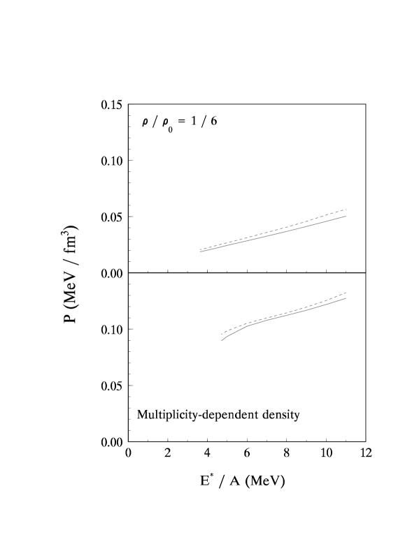
Figure 8: Pressure curves due to kinetic motion and Coulomb interaction (see Eq. 40) are plotted for the system of A=168 and Z=75 at fixed breakup density and multiplicity-dependent density. The dotted lines are calculated from the SMM85 while the ISMM presents the solid lines.

where $P$ is the pressure, $M$ is the total multiplicity, $V_{f}$ is the free breakup volume and $V$ is the total volume. Limiting the pressure estimates to temperatures for which the multiplicity exceeds 10 and the pressure can be more reasonably defined, we show the pressure corresponding to these multiplicity-dependent breakup densities in the lower panel of Fig. 8. The corresponding primary fragment multiplicities are shown in the lower panel of Fig. 9. Consistent with the conclusions of ref. dasgupta , we find the requirement of approximately constant interfragment spacing corresponds to breakup pressures that exhibit only a small fractional increase with temperature. In the upper panels, we show the corresponding caloric curves (Fig.7), pressures (Fig. 8), and multiplicities (Fig. 9) calculated at fixed breakup density $\rho/\rho_{0}=1/6$. These show a steeper dependence of the caloric curves on excitation energy and the small maximum displayed in the lower panel of Fig.7 at excitation energies of about 3 MeV disappears. The corresponding pressures at constant density, shown in the upper panel of Fig. 8, increase monotonically with excitation energy. However, they are lower than those calculated assuming a multiplicity dependent breakup density, because the density for the constant volume calculations is lower.

These figures reveal that the trends of the thermal dynamical properties of these three models to be similar. In general, the temperatures in the plateau region at $E^{\ast}/A=3-8$ MeV in the lower panel of Fig. 7 are larger for the ISMM calculations using the improved free excitation energies. This is consistent with the fact that the level densities and, consequently, the entropies of the fragments are lower in the improved model, which generally raises the temperature corresponding to a given excitation energy. Specifically in the plateau region, reducing the entropies of the fragments raises the latent heat for the transformation from excited fragments to nucleon gas and raises the temperature at which the transition occurs. The influence of the improved binding energies on the caloric curve is less obvious, but this change seems to be largely responsible for the differences between the SMM85 and ISMM at $E^{\ast}/A>6$ MeV.

Discussions of the nuclear caloric curve usually focus on the excitation energy dependence of the temperature and ignore the density dependence. To illustrate that the phase diagram is two dimensional and a density dependence does exist, we contrast in Fig. 10 the density dependence (right panel) of the temperature at a fixed excitation energy of $E^{\ast}/A=6MeV$ (open squares) to the excitation energy dependence (left panel) of the temperature at a fixed density of $\rho/\rho_{0}=1/6$ (solid circles). Both the excitation energy and the density dependences of the caloric curve are clearly important. It is therefore relevant to find and measure observables that constrain significantly the freezeout density.

IV.2 Charge and Mass Distributions

Calculations of the mass distribution (left panel) and charge distribution (right panel) for excited primary fragments are shown in Fig. 11 for a system with $A_{0}=186$ and $Z_{0}=75$ at $E^{\ast}/A=6MeV$. This system has the same charge to mass ratio as the symmetric ¹²⁴Sn+¹²⁴Sn system, but is chosen to be 3/4 of the total mass in order to approximately address the mass loss to preequilibrium emission. The dotted lines denote the predictions using SMM85 and the solid lines denote the predictions using ISMM. The primary distributions from ISMM fluctuate about the smooth distributions of SMM85 for $Z<20$ and $A<60$ and then fall below SMM85 at higher mass and charge. The fluctuations are related to the influence of shell and pairing effects on the ground state masses, which have no significant impact on the final yields after secondary decay as discussed below. The trend of reduced yields at higher masses and charges is related to the tendency shown in Fig. 1 for the binding energies in the SMM85 to consistently exceed the empirical values at $Z>20$ and $A>60$. Because conservation of mass and charge dictates that an increase in the yields of heavier fragments must be compensated by a decrease in the yields of the lighter ones, one should see a comparable under-prediction of the primary yields of the lighter fragments by SMM85.

Fig. 12 shows the corresponding final mass (left panel) and charge (right panel) distributions after secondary decay. The solid lines denote the predictions using ISMM. Experimental fragment yields from the central ${}^{124}Sn+^{124}Sn$ collisions are plotted as solid points txliu . To investigate the influence of the fluctuations in the primary distributions due to shell and pairing effects on the ground state masses, we have decayed the primary fragments from the SMM85 via the same empirical secondary decay procedure discussed in Sect. III. The final mass and charge distributions of the SMM85 are shown as the dashed lines in Fig. 13. Minimal discrepancies are seen in low mass and charge regime indicating that the secondary decay mechanism washes out the fluctuations in the primary distributions due to the influence of shell and pairing effects on the ground state masses. Meanwhile, significant differences on heavy fragments remain. In order to see the differences between the two calculations, the low A and Z regions are expanded in Figure 13. Here again, experimental fragment yields from the central ${}^{124}Sn+^{124}Sn$ collisions are plotted as solid points txliu . The agreement is very good even though no special attempt has been made to optimize the parameters of the calculations to achieve the best representation of the data.

IV.3 Isotopic distributions

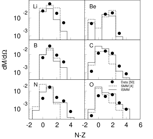
Figure 15: Isotopic distributions are shown for isotopes from Li to O. Experimental data are shown as the solid circles. The dashed lines denote calculations from the SMM code used in ref.williams97 and the solid lines are the final distributions obtained using the present ISMM model, which contains an empirical secondary decay procedure.

In Fig. 14, the primary isotopic distributions for four elements emitted are shown for a system with $A_{0}=186$ and $Z_{0}=75$ at $E^{\ast}/A=6$ MeV. The solid lines show predictions for the present improved model and the dashed lines show predictions of the SMM85 code of refs. smm ; Sneppen87 . The two calculations produce primary isotopic distributions that are considerably broader and more neutron rich than corresponding final distributions after secondary decay shown in Fig. 15. For reference, the measured isotopic distributions of refs. Xu00 ; txliu are shown as solid points in Fig. 15. While the parameters of the code were not optimized to reproduce the data, it is interesting to note that the widths of the distributions from ISMM calculations and data are similar although the data seem to be more neutron rich than the calculations. Studies have shown that the final isotopic distributions calculated with an empirical secondary decay procedure such as that employed by the ISMM are much broader and more neutron-rich than the corresponding distributions predicted by the more schematic statistical models Souza00 . In order to compare with the available experimental data, the isospin observables derived from these isotopic distributions such as isoscaling parameters Xu00 ; tsang01 ; Tan01 and isotopic temperatures require an accurate secondary decay approach with detailed nuclear structure information taken into account.

Isotope thermometers have been utilized as the primary probes for extracting the caloric curve of the nuclear liquid-gas phase transition. Since these observables are constructed from the isotopic distributions, they share the sensitivity to structure effects in the secondary decay discussed above. In the isotopic thermometer technique, the temperature is extracted from a set of four isotopes produced in multifragment breakups as follows Albergo ,

$$T_{iso}=\frac{\Delta B}{\ln(aR)}$$ (41)

where

$$R = \frac{Y(A_{1},Z_{1})/Y(A_{1}+1,Z_{1})}{Y(A_{2},Z_{2})/Y(A_{2}+1.Z_{2})},$$ (42)

$$\Delta B = B(A_{1},Z_{1})-B(A_{1}+1,Z_{1})$$ (43)

$$-B(A_{2},Z_{2})+B(A_{2}+1,Z_{2}),$$

and

$$a=\frac{\left(2J_{Z2,A2}+1\right)\left(2J_{Z1,A1+1}+1\right)}{\left(2J_{Z1,A1}+1\right)\left(2J_{Z2,A2+1}+1\right)}\left[\frac{A_{2}\left(A_{1}+1\right)}{A_{1}\left(A_{2}+1\right)}\right]^{3/2}.$$ (44)

Here $Y(A,Z)$ is the yield of a given fragment with mass A and charge Z; $B(A,Z)$ is the binding energy of this fragment; and $J_{Z,A}$ is the ground state spin of the nucleus. Although this expression is derived within the context of the grand canonical ensemble, it has been applied to a wide variety of reactions and regarded as an effective or “apparent” temperature that may differ somewhat from the true freezeout temperature $T$. The relationship between $T_{iso}$ and $T$ can be calculated within an appropriate statistical model for the fragmentation process if one exists. In general, one chooses a set of four isotopes with large $\Delta B$ to minimize sensitivity to details of the corrections from secondary decay.

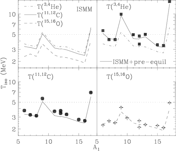
Figure 16: Isotopic temperatures extracted from three types of thermometers (see table 1). Experimental data are shown as the symbols. The lines are the calculations by the ISMM. For reference, the primary temperature of 5 MeV calculated from the ISMM is shown as the horizontal dotted lines. For details see text.

To examine the influence of secondary decay, measured and calculated temperatures are extracted from double ratios of Z=2-8 fragments and plotted in Figure 16. The large $\Delta B$ requirement generally limits the apparent temperature observables to three types of thermometers: a.) $T_{iso}(^{3,4}He)$, $Z_{2}$=2, $A_{2}$=3, b.) $T_{iso}(^{11,12}C)$, $Z_{2}$ =6, $A_{2}$=11, and c.) $T_{iso}(^{15,16}O)$, $Z_{2}$=8, $A_{2}$=15, where thermometer (a) involves the light particle pair ^3,4He while thermometers (b) and (c) concern only the intermediate mass fragments (IMF’s) of Z=3-8. Table I lists the corresponding thermometers plotted in Figure 16 . The top left panel in Fig. 16 shows the ISMM predictions for these three types of thermometers as a function of $A_{1}$.

Since the denominator in Eq. (42) is fixed by classifying the temperatures into three types, the fluctuations are related to $A_{1}$. In all cases, the two thermometers involving ¹⁰Be and ¹⁸O are much higher than the others due to many low lying states in these nuclei tsang97 . The extracted temperatures from all the other thermometers are significantly lower than the primary temperature of 5 MeV which is shown as the dotted line in the four panels. There seems to be a Z dependence in $T_{iso}$. $T_{iso}(^{15,16}O)$ is about 0.5 MeV lower than $T_{iso}(^{11,12}C)$ which is only slightly lower ($~{}0.2$ MeV) than $T_{iso}(^{3,4}He)$. In addition, there is also a trend of isotopic temperature values decreasing as a function of $A_{1}$. The lower temperatures reflect increasing contributions of multi-step secondary decay contributions. As these multi-step contributions originate from the decay from an ensemble of unstable nuclei that are less excited than the original ensemble, it has the effect of making the system appear cooler.

For comparison, we use the corresponding isotope temperatures extracted from the data obtained in the central collisions of ${}^{124}Sn+^{124}Sn$ reactions at E/A=50 MeV txliu shown as solid squares(top right panel), circles (bottom left panel) and stars (bottom right panel) for $T_{iso}(^{3,4}He)$, $T_{iso}(^{11,12}C)$, $T_{iso}(^{15,16}O)$, respectively in Figure 16. The calculated ISMM isotopic temperatures (lines) follow the trends of the corresponding experimental values. Despite the fact that the parameters in the ISMM calculations have not been optimized, the calculated temperatures of $T_{iso}(^{11,12}C)$ and $T_{iso}(^{15,16}O)$ (bottom panels) are nearly the same as the data within the theoretical uncertainties, which indicates that the IMF’s distributions can be well reproduced in an appropriate equilibrium model.

However, the experimental $T_{iso}(^{3,4}He)$ temperatures (solid squares in top right panel) are systematically higher than the corresponding ISMM values (dot dashed line). As these thermometers derive their sensitivity to the temperature from the large binding energy difference between ³He and ⁴He, the difficulty in reproducing these quantities may arise if there are significant nonequilibrium production mechanisms for light particles such as ³He xi98 ; xi98a . To illustrate this effect, we assumed that 2/3 of the measured ³He yield is of a non-thermal origin. This increases the ³He yield by a factor of three and the new calculations are shown as the solid line in the top right panel. The resulting apparent temperatures are nearly the same as the experimental data. This simple assumption explains the discrepancies between $T_{iso}(^{3,4}He)$ and $T_{iso}(^{11,12}C)$ observed experimentally. However, the present calculations also suggest that sequential decays have a much larger effects on $T_{iso}(^{11,12}C)$ and $T_{iso}(^{15,16}O)$ than previously assumed xi98 .

To illustrate the importance of using an accurate sequential decay code to decay the primary hot fragments before data can be accurately compared, Table I contains the experimental measured isotope temperatures in the fourth column. Predicted temperatures from the ISMM using the MSU-DECAY code are plotted in the fifth column. As shown in Figure 16 and Table I, there is a close correspondence in the fluctuations of the temperature between the ISMM and observed temperatures. However, if one uses the SMM code of Ref. [4], which contains a Fermi-break up decay mechanism for excited fragments and utilizes schematic structure information to calculate the secondary decays, the fluctuations in the temperature, listed in the last column in Table I, are much larger than those observed in the data. In this respect, one should especially note those involving ^8,9Li; ^9,10Be, ^12,13B, and ^17,18O where the calculated $T_{app}$ differ from the data by more than a factor of two. The discrepancies in the predicted ratios are significantly larger still, by a factor of $\Delta B/T_{iso}$, according to Eq. (41).

V Summary

The multifragmentation of excited nuclear systems produces excited fragments that decay into the observed ground state nuclei by mechanisms that are strongly influenced by the ground and excited state spins and energies of the fragments and by their decay branching ratios. Prior equilibrium multifragmentation models employed approximate descriptions for these quantities that are insufficiently accurate to describe the new isotopically resolved data now becoming available Xu00 ; txliu . In this paper, we include this information self-consistently, building the improved statistical multifragmentation model (ISMM) upon the foundations of ref. smm ; Sneppen87 . The main differences between the properties of the hot systems we calculate and those calculated in ref. smm ; Sneppen87 can be attributed to the more accurate expression for the binding energies that we employ; the structure of the low-lying states of the fragments plays little role in properties of the hot system. These structure effects become critical when the fragments cool later by secondary decay.

Our calculations call many of the previous conclusions of equilibrium multifragmentation models into question. In particular, we have found that the SMM85 and other similar calculations tended to overpredict the yields of heavy fragments, and, consequently, to underestimate those of the lighter ones. More importantly, we find that isotopic yields and observables like the isotopic temperatures require careful attention to the structure of the excited fragments. Thus, prior calculations of these isotopic observables using models that do not include such structure information accurately may be unreliable and lead to questionable conclusions.

Table 1: List of isotopic thermometers plotted in Figure 16.

IMF-meters	$\Delta B$	a	$T_{iso}$(Data)	$T_{iso}$(ISMM)	$T_{iso}$(SMM)[20]
6,7Li/11,12C	11.472	5.898	3.740	3.315	3.625
7,8Li/11,12C	16.690	5.361	3.244	3.212	4.419
8,9Li/11,12C	14.658	3.351	3.146	3.065	1.014
9,10Be/11,12C	11.910	1.028	5.643	5.102	12.561
11,12B/11,12C	15.352	3.000	3.651	3.154	3.928
12,13B/11,12C	13.844	5.278	3.720	3.031	1.636
12,13C/11,12C	13.776	7.917	3.418	3.078	3.608
13,14C/11,12C	10.545	1.962	3.288	2.949	2.590
15,16N/11,12C	16.233	9.669	2.767	2.564	2.716
16,17O/11,12C	14.578	23.069	2.648	2.443	2.555
17,18O/11,12C	10.678	0.637	6.921	6.009	4.514
6,7Li/15,16O	8.413	3.050	2.273	2.352	2.209
7,8Li/15,16O	13.631	2.773	2.636	2.565	3.084
8,9Li/15,16O	11.599	1.733	2.476	2.368	0.768
9,10Be/15,16O	8.851	0.532	4.143	3.610	5.562
11,12B/15,16O	12.293	1.551	2.906	2.466	2.701
12,13B/15,16O	10.785	2.729	2.109	2.303	1.184
12,13C/15,16O	10.717	4.094	2.643	2.334	2.402
13,14C/15,16O	7.486	1.014	2.316	2.270	1.588
15,16N/15,16O	13.174	5.000	2.236	2.043	1.990
16,17O/15,16O	11.519	11.930	2.083	1.893	1.814
17,18O/15,16O	7.619	0.330	4.863	4.027	2.523
6,7Li/3,4He	13.328	2.183	5.693	3.632	4.708
7,8Li/3,4He	18.546	1.984	4.197	3.431	5.386
8,9Li/3,4He	16.514	1.240	4.200	3.309	1.169
9,10Be/3,4He	13.766	0.380	9.938	5.413	22.410
11,12B/3,4He	17.208	1.110	4.948	3.390	4.814
12,13B/3,4He	15.700	1.953	3.599	3.287	1.931
12,13C/3,4He	15.632	2.930	4.731	3.337	4.487
13,14C/3,4He	12.401	0.726	5.000	3.276	3.319
15,16N/3,4He	18.089	3.578	3.519	2.766	3.206
16,17O/3,4He	16.434	8.536	3.439	2.661	3.059
17,18O/3,4He	12.534	0.236	15.334	6.311	6.170

Figure 1: Differences between the total binding energies predicted by mass formulae and those recomended in ref. Audi95 . Upper panel :Plot (a) displays the differences when one uses the LDM mass formula used in SMM85 calculations. Sneppen87 . Lower panel: Plot (b) displays the differences when one uses the ILDM mass formula presented in this work.

Figure 2: Total binding energies for various nuclei. The full lines correspond to the corrected LDM formula, whereas the symbols represent the experimental data of ref. Audi95 . The dashed lines correspond to the predictions given by Eq. (11) using the optimized parameters. For details see the text.

Figure 3: Internal free energies for $A=20$ (upper panel) and $A=200$ (lower panel). The SMM85 expression [Eq. (16)] is represented by the full line whereas the dashed lines stand for the results obtained with the Taylor expansion [Eq. (18)]. The Free energy calculated through the level density given by Eq. (20) is depicted by the symbols.

Figure 4: Level densities as a function of excitation energy for ²⁰Ne and ³¹P. Two energy ranges are plotted to show the behaviors of level densities at both low (left panels) and high energy (right panels) ends. The density of experimentally known levels is shown as bars in the low energy region. The dashed lines are the extrapolations of the empirical values according to Eq. 25. The dotted lines are the level density (Eq. 20) parametrized from the SMM85. The solid lines are the level density adopted in this work (Eqs. 31-34).

Figure 5: Comparison between $F^{*}(T)$ calculated through Eqs. (17) and (31)-(34), symbols, and the approximation given by Eq. (35), full line. To illustrate the influence of quantum effects at low temperatures, the dashed line represents the free energy used in SMM85 calculations Eq. (16). For details see text.

Figure 6: Best fit values of $T_{0}$ for different nuclei (symbols). The dashed line corresponds to Eq. 36 used for $Z>15$.

Figure 7: Caloric curves are shown for calculations of the system of A=168 and Z=75 at fixed breakup density and multiplicity-dependent density. The dotted lines are calculated from the SMM85. The dashed lines result when empirical binding energies are taken into account. The solid lines are obtained from the improved model, ISMM, with empirical modifications of both binding energies and free energies.

Figure 9: Average breakup multiplicities are shown for the system of A=168 and Z=75 at fixed breakup density and multiplicity-dependent density. The dotted lines are calculated from the SMM85 while the ISMM presents the solid lines.

Figure 10: Dependences of temperature on excitation energy and breakup density are shown for the system of A=168 and Z=75. Calculations as function of excitation energy at fixed density of 1/6 normal density are shown as solid circles in the left panel. Calculations as function of density at fixed excitation energy are shown as open squares in the right panel.

Figure 11: Mass and charge distributions for the system of A=186 and Z=75. The dashed lines are the calculations from the SMM85. The solid lines are calculated using the improved model ISMM.

Figure 12: Final mass and charge distributions after applying MSU-DECAY, the empirical secondary decay procedure discussed in Sect. III. The dashed lines are calculated from the primary results of the SMM85 while the solid lines are from ISMM.

Figure 13: Final mass and charge distributions from ISMM (solid lines) and SMM85 (dashed lines) are shown. For reference, some measured data from refs. Xu00 ; txliu are plotted as solid circles.

Figure 14: Primary isotopic distributions for Be, C, O and Ne nuclei. The dashed lines correspond to the calculations of the SMM85 while the solid lines represent the results of ISMM.