Kaon and Lambda Production at Intermediate $p_{T}$: Insights into the Hadronization of the Bulk Partonic Matter Created in Au+Au Collisions at RHIC

Abstract

Measurements of identified particles over a broad transverse momentum $p_{T}$ range may provide particularly strong evidence for the existence of a thermalized partonic state in heavy-ion collisions (i.e. a quark-gluon plasma). Of particular interest are the centrality dependence and the azimuthal anisotropy in the yield of baryons and mesons at intermediate $p_{T}$. The first measurements of $v_{2}$ — an event-by-event azimuthal anisotropy parameter — and the nuclear modification factor $R_{CP}$ for mid-rapidity $K_{S}^{0}$ and $\Lambda+\overline{\Lambda}$ production in Au+Au collisions at ultra-relativistic energy are presented. The $K_{S}^{0}$, $\Lambda$, and $\overline{\Lambda}$ candidates are selected based on characteristics of their decays in the STAR Time Projection Chamber (TPC). A statistical treatment is used to extract $v_{2}(p_{T})$ and $R_{CP}(p_{T})$ from their invariant mass distributions. These measurements establish the particle type dependence of $v_{2}$ and $R_{CP}$ in the kinematic region $0.4<p_{T}<6.0$ and $|y|<1.0$.

In the low $p_{T}$ region ($p_{T}<1.0$ GeV/c) the $v_{2}$ values for different particles are increasing with $p_{T}$ and follow a mass dependence similar to that expected from hydrodynamical models of Au+Au collisions — where, at a given $p_{T}$, the particle with the larger mass will have a smaller $v_{2}$. At higher $p_{T}$ however, $v_{2}$ of the heavier $\Lambda$ hyperon continues to increase while $v_{2}$ of the lighter $K_{S}^{0}$ meson saturates at $v_{2}\sim 0.13$ for $2.0<p_{T}<5.0$ GeV/c. At intermediate $p_{T}$ the $v_{2}$ of $K_{S}^{0}$ and $\Lambda+\overline{\Lambda}$ are shown to follow a number-of-constituent-quark scaling with $\frac{v_{2}^{kaon}(p_{T}/2)}{2}\approx\frac{v_{2}^{lambda}(p_{T}/3)}{3}$.

The binary collision scaled centrality ratio $R_{CP}$ shows that $\Lambda+\overline{\Lambda}$ production at intermediate $p_{T}$ increases more rapidly with system size than kaon production: This is consistent with a scenario where multi-parton dynamics play an important role in particle production. At $p_{T}\approx 5.5$ GeV/c $\Lambda+\overline{\Lambda}$, $K_{S}^{0}$, and charged hadron production are all suppressed by a similar amount: a factor of three below expectations from binary nucleon-nucleon collision scaling (i.e. $R_{CP}\approx 0.33$). This $p_{T}$ value establishes the extent to which the centrality dependent enhancement of baryon production persists.

The particle-type dependence of $v_{2}$ and $R_{CP}$ provides a stringent test for models of heavy-ion collisions. In particular the larger values of $\Lambda+\overline{\Lambda}$ $v_{2}$ compared to their smaller suppression manifested in $R_{CP}$ suggests that for $p_{T}<4.0$ GeV/c a particle production mechanism beyond the framework of energy loss and fragmentation exists in central Au+Au collisions. The particle- and $p_{T}$-dependence of $v_{2}$, and $R_{CP}$ are consistent, however, with expectations based on the hadronization of a bulk partonic matter by coalescence or recombination. As such, the constituent-quark-number scaled $v_{2}$ reflects the anisotropy established in a partonic stage and provides strong evidence for the existence of a quark-gluon plasma in Au+Au collisions at RHIC.

Physics 2003 Charles A. Whitten Jr. Huan Z. Huang Charles Buchanan An Yin Nu Xu To my family, whose unceasing hard work, effort and diligence have given me advantages that made it possible for me to pursue this goal and to my friends, whose support throughout my life gave me the strength, confidence and character to complete it.

Chapter 0 Introduction to Relativistic Heavy-Ion Collisions

By colliding heavy nuclei at relativistic energies scientists are able to test the nature of nuclear matter at high temperature and density, to produce conditions similar to those thought prevalent in the early universe, and to search for previously unstudied states of nuclear matter. In this chapter, we discuss the essential components of the theory thought to govern heavy-ion collisions, and we introduce the analysis topics that will be presented in this thesis.

1 QCD–Asymptotic Freedom and Confinement

Matter is made of leptons, quarks, and force mediators. Quarks, the building blocks of nucleons (and all hadronic matter), carry a property analogous to electric charge called color. The theory that describes the forces between colored objects and that is thought to be the correct theory for strong interaction is called quantum chromodynamics (QCD). In QCD, just as the electromagnetic force is carried by photons, the color force (or strong force) is carried by gluons. However, whereas photons carry no electric charge, gluons do carry color charge so they can interact directly with each other, and whereas the electrodynamic coupling constant $\alpha=\frac{1}{137}$, the strong coupling constant $\alpha_{s}$ can be larger than one. As a consequence of the direct gluon-gluon coupling the effective coupling constant for the strong force becomes smaller at shorter distances. This effect is known as asymptotic freedom. Asymptotic freedom means the force between quarks is stronger at larger distances so quarks seem to remain confined to a small ($\sim$1 fm³) region in colorless groups of two (mesons) or three (baryons). Because the effective strong coupling is only small at short distances, perturbation theory can only be used with QCD for interactions involving large momentum transfers (i.e. hard processes). Although perturbative QCD (pQCD) is in very good agreement with experimental observations involving hard processes (see Figure 1 for example [GG00]), it cannot be used to calculate QCD predictions for the processes that dominate the universe at present: soft processes

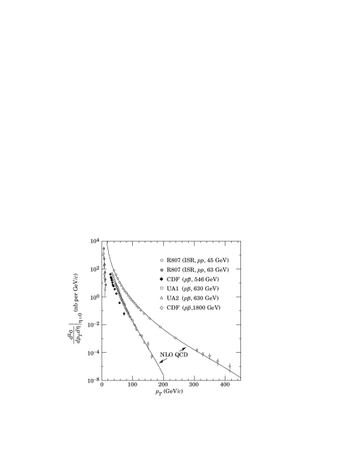
Figure 1: Differential cross-sections for single jet production at pseudo-rapidity $\eta=0$ as a function of the jet transverse momentum $p_{T}$ in proton (anti-)proton collisions. Jets are somewhat collimated sprays of particles produced when quarks or gluons collide, transfer (and carry away) a lot of momentum, and then fragment into a spray of hadrons. The curves represent pQCD calculations for the collisions at center-of-mass energy $\sqrt{s}=630$ and 1800 GeV.

Explicit QCD Lagrangian calculations of the force between quarks can only be made in the limits of weak and strong coupling. To understand the behavior of colored objects where pQCD is not a valid approximation, physicists rely on numerical path integrals of the QCD Lagrangian on a discretized lattice in four-dimensional Euclidean space-time. It is the formulation of Lattice QCD with a strong coupling approximation that first demonstrated how quarks are confined [Wil74].

In principle, the lattice formulation of QCD can be used to perform numerical calculations for all physical regimes. In practice, however, there are regimes where approximations used to simplify the calculations fail and the computations become technically very challenging.

2 Deconfined Quark Matter

In the strong coupling regime the energy required to separate two quarks increases linearly with the distance between them. As a result, we have never observed deconfined quarks: a deconfined quark is taken as one that can move in a volume much larger than the volume of a proton. Recent advances in the formulation of thermodynamical lattice QCD at finite temperature and density however, suggests that when sufficiently high temperature and density are reached, quarks become effectively deconfined. Figure 2 [Kar02] shows that the ratio of the energy density scaled by $T^{4}$ (where $T$ is the system temperature) $\epsilon/T^{4}$ quickly increases at a critical temperature $T_{C}$. The magnitude of $\epsilon/T^{4}$ reflects the number of degrees of freedom in the thermodynamic system. The rise corresponds to a transition in the system to a state where the quarks and gluons have become relevant degrees of freedom.

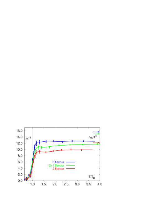
Figure 2: The energy density in QCD from lattice calculations. When the temperature $T$ reaches the critical temperature $T_{c}$, the number of degrees of freedom rapidly rises indicating that quarks and gluons become relevant degrees of freedom. The arrows represent the Stefan-Boltzmann values for asymptotically high temperature.

The idea of a new state of matter where deconfined quarks and gluons are the relevant degrees of freedom is not new. In 1973, shortly after asymptotic freedom was shown to arise from QCD theory [GW73, Pol73], deconfined quark matter was postulated as the true state of nuclear matter at high energy density at the center of neutron stars [CP75]:

A neutron has radius of about 0.5–1 fm, and so has a density of about $8\times 10^{14}$ gm/cm³, whereas the central density of a neutron star can be as much as $10^{16}-10^{17}$ gm/cm³. In this case, one must expect the hadrons to overlap, and their individuality to be confused. Therefore, we suggest that there is a phase change, and that nuclear matter at such high densities is a quark soup.

Later, in the fall of 1974, at a workshop on heavy-ion collisions, T.D. Lee discussed the need for a physics program to study quark matter [Lee75]:

Hitherto, in high-energy physics we have concentrated on experiments in which we distribute a higher and higher amount of energy into a region with smaller and smaller dimensions. In order to study the question of “vacuum,” we must turn to a different direction; we should investigate some “bulk” phenomena by distributing high energy over a relatively large volume.

Figure 3: The energy density $\epsilon$ and pressure $P$, scaled by $T^{4}$ from a statistical model [RL03]. The various lines show results for different hadron mass spectra. The results show an increase in the energy density degrees of freedom at a critical temperature near $T=158$ MeV.

Not all conceptualizations of the cross-over from hadronic degrees of freedom to a new form of matter relied on QCD or the knowledge of quarks. In 1951, Pomeranchuk postulated an upper limit to the temperature of hadronic matter based on the finite size of hadrons [Pom51]. In the late sixties, Hagedorn’s approach involving a self-similar hadronic resonance composition pointed to a similar limit [Hag65]. We now believe these limits reflect a transition to a state of matter with quarks and gluons as deconfined constituents. Figure 3 shows the scaled energy density $\epsilon/T^{4}$ and scaled pressure $P/T^{4}$ derived from a statistical model of a hadronic gas [RL03].

3 Goals of Heavy-Ion Physics

The creation and study of bulk matter made of deconfined quarks and gluons (i.e. a quark-gluon plasma or QGP) was one of the prime motivations for building the Relativistic Heavy-Ion Collider (RHIC). The interaction of high-energy, colliding beams of heavy nuclei generates matter of extreme density and temperature. The temperatures and densities reached are expected to be similar to those thought to have prevailed in the very early universe, prior to the formation of protons and neutrons. The observation and study of matter in these conditions will be relevant to the nuclear physics community, the astrophysics community and the high-energy physics community. One also expects this research to have a significant impact on many in the general public since the nature of our universe at the earliest stages and the transitions that produced the matter we are familiar with today are interesting to most naturally curious or inquisitive people.

By colliding large nuclei at high energy a window is opened onto an asymptotic regime of QCD. The exploration of this region of the QCD phase diagram is an exciting scientific endeavor. Many questions will be addressed in heavy-ion research programs: How well does the system thermalize? In the early universe, how did matter hadronize? Is there a first order phase transition, second order phase transition or smooth cross-over? How is fragmentation affected by the dense system created in the collisions? What is the role of chiral symmetry breaking in the transition from deconfined partons to hadrons? The measurements presented here provide insight into how well the matter created at RHIC thermalizes and how it subsequently hadronizes.

Learning about dense nuclear matter is also important to the astrophysics community. Heavy-ion physics can potentially provide insight into the structure of neutron stars (i.e. their mass-radius relationship, their thermal evolution, their upper mass limit). In addition, reaching a better understanding of dense nuclear matter will help determine whether a new class of stars, quark stars, are likely or unlikely to exist in our universe.

Perhaps the most exciting discoveries made will be those that are least expected. The heavy-ion collisions at RHIC constitute an exploration into the unknown and one should be ready to be surprised. We do not know, for example, what, if any, exotic states may be produced in the hadronization of bulk quark matter. Candidates include multi-quark states, exotic atoms, and large droplets of strange-quark matter.

4 Experimental Observations

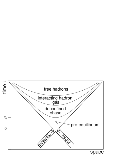
Figure 4: A sketch of the expected evolution of a relativistic heavy-ion collision.

Figure 1 depicts the space-time evolution of a heavy-ion collision. Four possible stages of the evolution are shown: a pre-equilibrium stage, an equilibrated-deconfined-parton stage, an interacting-hadron-gas stage and finally a free-hadrons stage. The experiments at RHIC detect hadrons in the free-hadron stage of the collision evolution. Probing the early stage of the collision evolution with particles measured in this final stage is a significant challenge. In this thesis we will present measurements thought to be sensitive to the early part of the collision evolution and to a possible deconfined-parton phase.

1 Initial Conditions

It is not known a-priori that an equilibrated-deconfined-parton phase can be created by colliding heavy ions in the laboratory. The large energy densities reached in central collisions (i.e. head-on collisions) however, significantly surpass estimates of the energy densities needed to reach the deconfinement phase transition. The initial energy density $\epsilon$ of the produced medium can be determined using the Bjorken estimate [Bjo83]

$$\epsilon=\left(\frac{dN_{h}}{dy}\right)_{y=0}\frac{w_{h}}{\pi R_{A}^{2}\tau_{0}},$$ (1)

where $(\frac{dN_{h}}{dy})_{y=0}$ is the number of hadrons per unit rapidity produced at mid-rapidity, $w_{h}$ is the average energy of the hadrons, $R_{A}$ is the nuclear radius, and $\tau_{0}$ is the formation time of the medium. The formation time is not known but is generally taken to be approximately one fm/c. The density of normal nuclear matter is approximately $0.16$ GeV/fm³. Lattice calculations predict that the phase transition to deconfined quarks and gluons occurs near 1.0 GeV/fm³. The Bjorken estimate for the initial energy density in central Pb+Pb collisions with $\sqrt{s_{{}_{NN}}}=17$ GeV at the CERN-SPS experiment is 3.5 GeV/fm³ [Sat03]. The estimate from RHIC for central Au+Au collisions at $\sqrt{s_{{}_{NN}}}=130$ GeV is 4.6 GeV/fm³ [Zaj02]. For the top RHIC energy ($\sqrt{s_{{}_{NN}}}=200$ GeV), $\epsilon\sim 5.0$ GeV/fm³ [DE03]. These estimates of $\epsilon$ far exceed the energy density thought necessary to generate deconfined partonic matter. Given these large densities, collective behavior due to multiple interactions is expected. An important question to ask then is; are the interactions copious enough and rapid enough to thermalize the dynamic and expanding matter created in the laboratory? Answering this question will be a challenge to the experiments at RHIC. Figure 5 (left) shows how the rapidity density per participating nucleon pair increases as a function of $\sqrt{s_{{}_{NN}}}$ [Baz03].

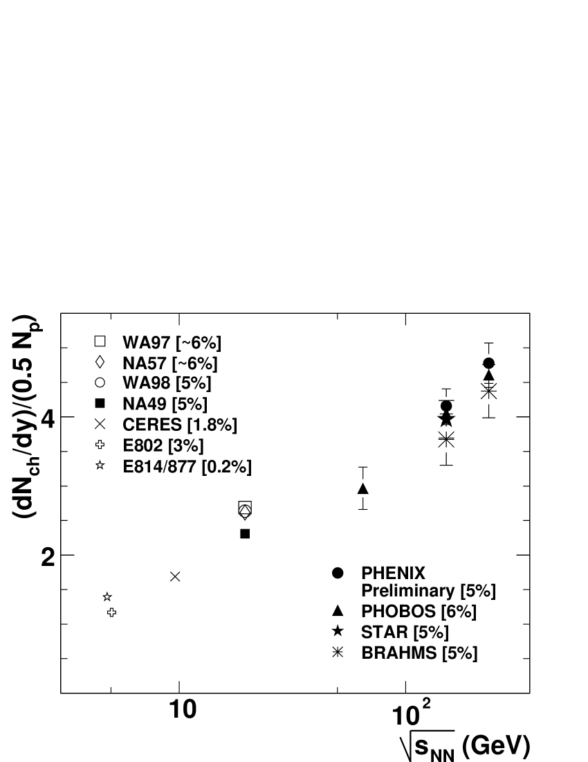
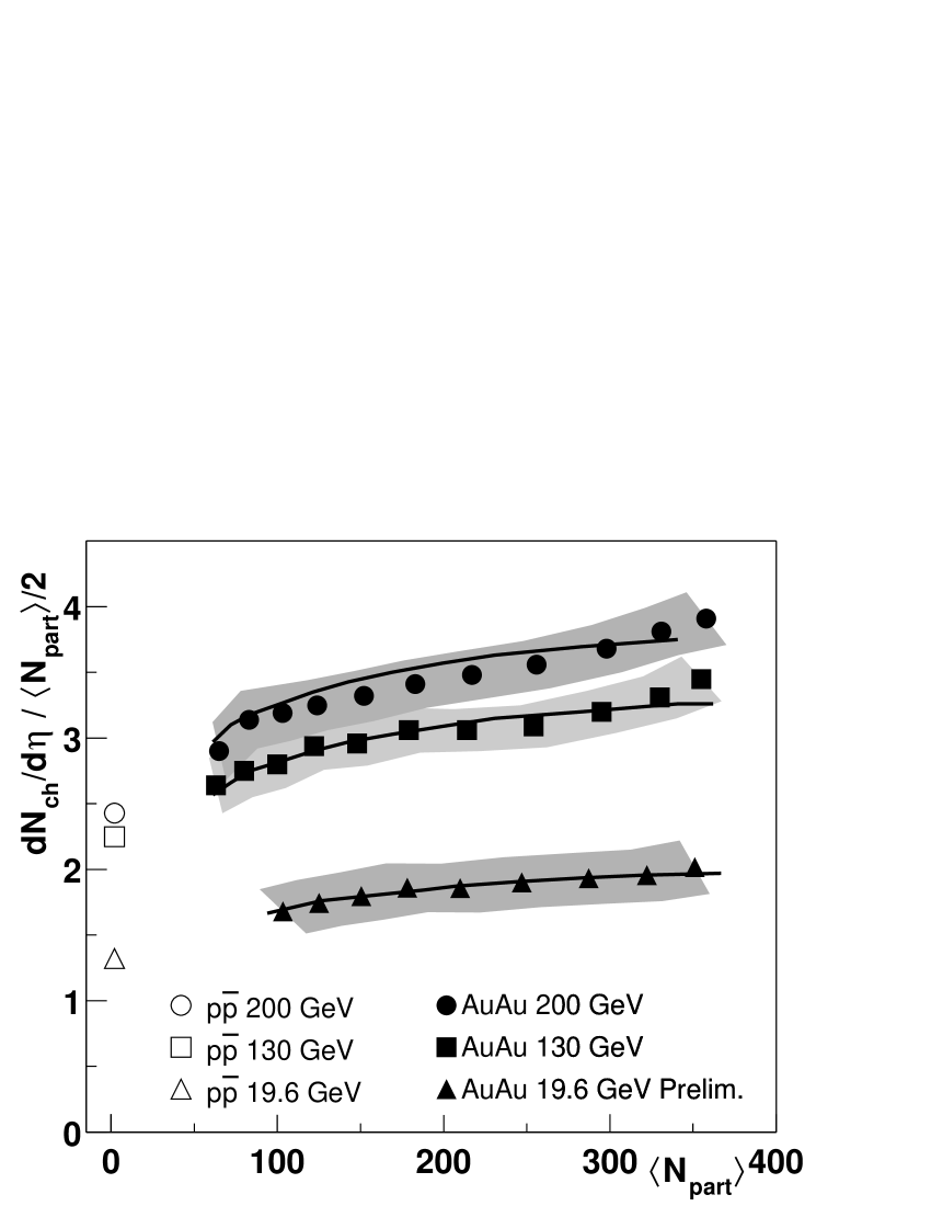
Figure 5: Left: Charged particle rapidity density at mid-rapidity scaled by the number of participating nucleon pairs $0.5\times$ N_part versus $\sqrt{s_{{}_{NN}}}$ [Baz03]. Right: Scaled pseudo-rapidity density for Au+Au and p+p collisions at $\sqrt{s_{{}_{NN}}}=$ 19.6, 130, and 200 GeV versus N_part [Bac03b].

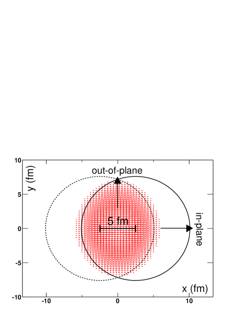
Figure 6: The overlap density for Au nuclei colliding off-axis. The beam directions are in and out of the of the page. The two large circles represent the outline of the incoming or outgoing Au nuclei. The impact parameter b—the distance between the center of the two colliding nuclei in the azimuthal plane—is 5 fm. The reaction plane is by the beam axis and the vector connecting the centers of the two nuclei.

In addition to the center-of-mass energy $\sqrt{s_{{}_{NN}}}$, the initial conditions of heavy-ion collisions also depend on the centrality of the collision. An off-axis nucleus-nucleus collision will have a smaller number of participating nucleons (N_part), a smaller system size, and a smaller initial energy density. Figure 5 (right) shows the rapidity density per participating nucleon pair versus N_part [Bac03b]. We also note that for nuclei colliding off-axis, the overlap region will be asymmetric. In Figure 6 we plot the overlap density for Au nuclei colliding with impact parameter b = 5 fm. A Woods-Saxon distribution is used for the density profile of the Au nuclei.

Most observables in heavy-ion collisions are integrated over the azimuthal angle and, as such, they are insensitive to the azimuthal asymmetry of the initial source. In this thesis we discuss measurements sensitive to the conversion of the initial spatial anisotropy to a final momentum-space anisotropy. The spatial anisotropy can be quantified by estimating the eccentricity $\varepsilon$ of the initial source,

$$\varepsilon=\frac{\langle y^{2}-x^{2}\rangle}{\langle y^{2}+x^{2}\rangle}.$$ (2)

Extracting the mean eccentricity of the initial source $\langle\varepsilon\rangle$ for a given centrality interval is helpful for understanding the event-by-event anisotropy in the final state momentum distributions. Analytic of initial eccentricities can be found in Appendix 5.

2 Event-by-event Momentum-space Anisotropy

Anisotropy in the distribution of a particle in momentum-space is thought to be sensitive to the early stage of the collision system. The anisotropy of the source will be largest immediately after the collision occurs. As the system evolves, the spatial anisotropy is converted by multiple interactions into a momentum-space anisotropy. With time, the interactions will cause the spatial distribution to become more isotropic. For this reason, it’s believed that the final azimuthal momentum-space anisotropy is primarily built up in the initial moments of the system’s evolution. Figure 7 shows the evolution of the source shape calculated from a model where the collision system is described by hydrodynamic equations [KSH00].

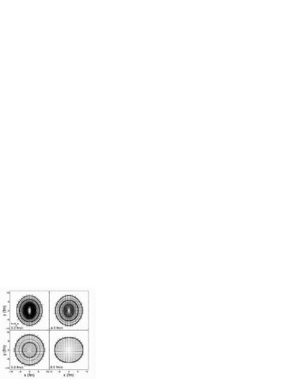
Figure 7: The evolution of the source shape is shown from a model where a heavy-ion collision is treated as a hydrodynamic system [KSH00]. The initial shape is extended out-of-plane. By 8 fm/c after the formation time ($\tau-\tau_{0}$), the shape has deformed to an in-plane extended source. In this model, the anisotropy in momentum-space measured by $v_{2}$ is dominated by the early stages.

The azimuthal anisotropy of the transverse momentum distribution for a particle can be described by expanding the azimuthal component of the particle’s momentum distribution in a Fourier series,

$$\frac{d^{3}n}{p_{T}dp_{T}dyd\phi}=\frac{d^{2}n}{p_{T}dp_{T}dy}\left[1+2\sum_{\alpha}{v_{\alpha}\cos\left(\alpha[\phi-\Psi_{RP}]\right)}\right].$$ (3)

The harmonic coefficients, $v_{\alpha}$, are anisotropy parameters, $p_{T}$, $y$, and $\phi$ are the respective transverse momentum, rapidity, and azimuthal angle for the particle, and $\Psi_{RP}$ is the reaction plane angle [PV98]. The second coefficient $v_{2}$ (customarily called elliptic flow) measures the elliptic component of the anisotropy. Due to the shape of the source created in an off-axis collision, $v_{2}$ is the largest and most studied of the anisotropy parameters.

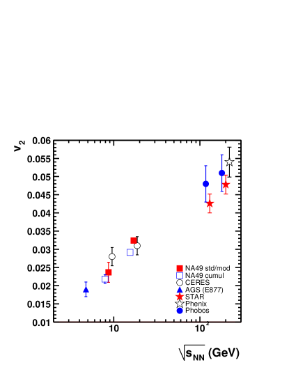
Figure 8: The integrated anisotropy parameter $v_{2}$ near mid-rapidity for mid-central events (roughly 12–34% central) plotted versus collision energy [Alt03].

Figure 8 shows the energy dependence of $v_{2}$ for charged particles near mid-rapidity. For this energy range $v_{2}$ is positive and rising monotonically with the nucleon-nucleon center of mass energy. At lower energies $v_{2}$ is negative [Ada02].

Multiple interactions are necessary to develop a momentum-space anisotropy from a coordinate-space anisotropy. If each nucleon-nucleon collision is independent, the final momentum distribution will represent a superposition of random collisions and will therefore be isotropic. The azimuthal momentum-space distribution of charged hadrons with $2.0<p_{T}<6.0$ GeV/c, for three centrality intervals, is shown in Figure 9 (left). Figure 9 (right) shows how $v_{2}$ for charged hadrons changes with $p_{T}$ (differential $v_{2}$). The magnitude of $v_{2}$ is smallest in central events because the initial eccentricity $\varepsilon$ is smaller.

The large saturated values of $v_{2}$ at high $p_{T}$ are a surprising result from RHIC. Although hydrodynamic models predict a monotonic increase of differential $v_{2}$, it is believed that hydrodynamic models must fail at higher values of $p_{T}$ where their assumptions become invalid. The measurement of a large $v_{2}$ at high $p_{T}$ gives rise to the question: “how does the initial spatial anisotropy manifest itself in the distribution of high $p_{T}$ particles?” One explanation is that high energy partons lose energy as they pass through the matter created in the collisions. Since the source is asymmetric, the amount of energy loss will depend on the direction the parton travels. As such, energy loss can lead to a momentum-space anisotropy that reflects the initial spatial anisotropy of the source. We will discuss energy loss and the suppression of high $p_{T}$ particle production in section 3.

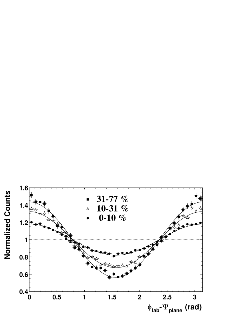
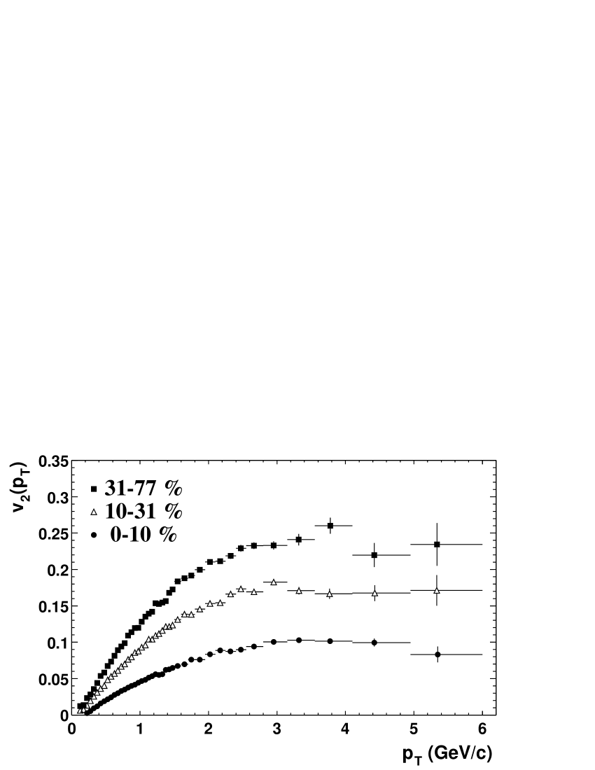
Figure 9: Left: The distribution of charged particles with $2.0<p_{T}<6.0$ GeV/c in the azimuthal plane from Au+Au collisions at $\sqrt{s_{{}_{NN}}}=130$ GeV. The 0-10%, 10-31%, and 31-77% represent different classes of centrality where 0-10% is the most central. Right: The differential $v_{2}$ for in three centrality intervals [Adl03a].

Figure 10 shows the differential $v_{2}$ at mid rapidity for identified particles at low $p_{T}$ ($p_{T}<1$ GeV/c) where particles can be identified by their energy loss in the detector gas [Adl01]. The hydrodynamic models predict a mass-ordering for elliptic flow with less massive particles having larger elliptic flow for all values of $p_{T}$.

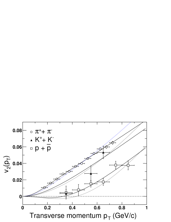
Figure 10: The differential elliptic flow for identified particles at mid-rapidity from Au+Au collisions at $\sqrt{s_{{}_{NN}}}=130$ GeV [Adl01]. The curves represent fits to hydrodynamic inspired parameterizations.

The large $v_{2}$ and its mass-ordering at low $p_{T}$ are consistent with the hydrodynamic limit for the conversion of spatial anisotropy to momentum anisotropy (where local thermal equilibrium has been assumed) [HKH01, Oll92, Sor99, TLS01]. At intermediate $p_{T}$ ($1.5<p_{T}<4$ GeV/c), however, while hydrodynamic models predict a monotonic increase, the charged hadron $v_{2}$ saturates at a value approximately independent of $p_{T}$. After the first year of RHIC data taking, the particle-type dependence of $v_{2}$ in the high momentum region remained an open question. In this thesis we present measurements of $v_{2}$ for $K_{S}^{0}$ and $\Lambda+\overline{\Lambda}$ at mid-rapidity from Au+Au collisions at $\sqrt{s_{{}_{NN}}}=200$ GeV/c that extend up to $p_{T}\sim 6$ GeV/c.

3 Nuclear Modification of Particle Production

Like $v_{2}$, high $p_{T}$ hadron production—presumably through scatterings of partons involving large momentum transfer—is also thought to probe the early stage of heavy-ion collisions. High-energy partons passing through dense matter are predicted to lose energy by induced gluon radiation [GP90, BSZ00, GVW03]. Since the total energy loss depends on the color charge density of the medium, nuclear modification of the high $p_{T}$ particle yields can probe the dense, perhaps deconfined-partonic matter created by the collision.

Partonic energy loss or jet-quenching can be studied by measuring the modification of particle production in nuclear collisions. A nuclear modification factor can be formed by taking the ratio of the particle yields in nucleus-nucleus collisions and the particle yields in proton-proton collisions. The ratio is then scaled by $T_{AA}=\langle\mathrm{N_{binary}}\rangle/\sigma^{NN}_{inel}$ to account for the trivial increase in the yield with the system size:

$$R_{AA}(p_{T})=\frac{d^{2}n^{AA}/dp_{T}d\eta}{T_{AA}d^{2}\sigma^{NN}/dp_{T}d\eta},$$ (4)

where $\eta$ is the pseudo-rapidity and $\mathrm{N_{binary}}$ is the number of binary nucleon-nucleon collisions. In the absence of nuclear effects, at high $p_{T}$, $R_{AA}$ is expected to be unity. In the low $p_{T}$ region the yield is not expected to scale with $\mathrm{N_{binary}}$. The $p_{T}$-scale where the high $p_{T}$ regime begins is an experimental observable that our measurements will address.

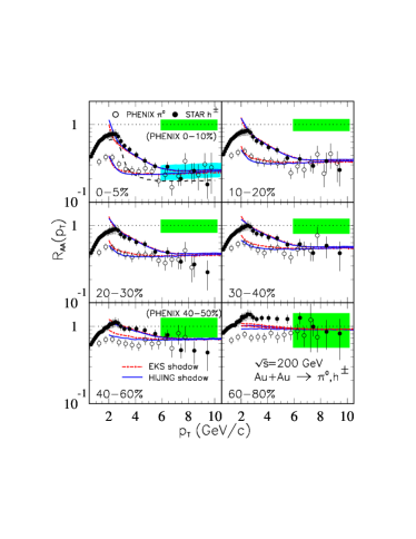
Figure 11: The nuclear modification parameter $R_{AA}$ for charged hadrons [Ada03b] and for neutral pions [Adl03f] in Au+Au collisions at $\sqrt{s_{{}_{NN}}}=200$ GeV. The panels show different Au+Au collision centrality intervals with the most central in the top left. The curves show model calculations based on partonic energy loss and other nuclear effects [Wan03].

Figure 11 shows $R_{AA}$ for charged hadrons and neutral pions $\pi^{0}$ from Au+Au collisions at $\sqrt{s_{{}_{NN}}}=200$ GeV. The high $p_{T}$ yields in central Au+Au collisions are suppressed with respect to $\mathrm{N_{binary}}$ scaling. The suppression is largest for central collisions while the yields in peripheral collisions are consistent with expectations from $\mathrm{N_{binary}}$ scaling. The suppression is approximately independent of $p_{T}$ for $p_{T}>3$ GeV/c for $\pi^{0}$ and for $p_{T}>5$ GeV/c for charged hadrons.

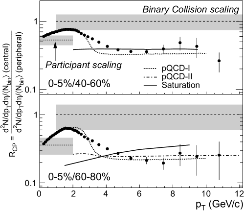
Figure 12: Nuclear modification of charged particle production measured at $\sqrt{s_{{}_{NN}}}=200$ GeV from central Au+Au events (0–5% of the collision cross-section) compared to peripheral Au+Au events (40–60% and 60–80% of the collision cross-section) [Ada03b].

Like $R_{AA}$, the ratio of the yields in central and the yields in peripheral collisions ($R_{CP}$) also can measure nuclear modifications to particle production:

$$R_{CP}(p_{T})=\frac{\left[dn/\left(\mathrm{N_{binary}}dp_{T}\right)\right]^{\mathrm{central}}}{\left[dn/\left(\mathrm{N_{binary}}dp_{T}\right)\right]^{\mathrm{peripheral}}}.$$ (5)

When $R_{AA}$ for peripheral events follows $\mathrm{N_{binary}}$ scaling, $R_{CP}\approx R_{AA}^{central}$. The ratio $R_{CP}$ typically has smaller systematic uncertainties than $R_{AA}$ and does not require the measurement of a p+p reference spectrum. The charged hadron $R_{CP}$ in Figure 12 shows a suppression of particle yields in central events compared to scaled peripheral events. The suppression of charged hadrons is roughly constant for $p_{T}>5$ GeV/c. The dependence on particle-type of the suppression and the $p_{T}$-scale for its onset remained an open question after the first year of RHIC collisions. In this thesis we present the measurement of $R_{CP}$ for $K_{S}^{0}$ and $\Lambda+\overline{\Lambda}$ from Au+Au collisions at $\sqrt{s_{{}_{NN}}}=200$ GeV up to $p_{T}\sim 6$ GeV/c.

As mentioned in section 2, energy loss can also manifest itself in $v_{2}$. By suppressing the yield of large $p_{T}$ particles more in the out-of-plane direction than the in-plane direction, energy loss can cause an anisotropy in the final momentum distribution. The particle-type dependence of $v_{2}$ and $R_{CP}$ will be a powerful test of the energy loss hypothesis. If energy loss governs the development of $v_{2}$ and $R_{CP}$ then we expect either no particle-type dependence or we expect the particle with the larger $v_{2}$ to also have a larger suppression.

4 Other Observations

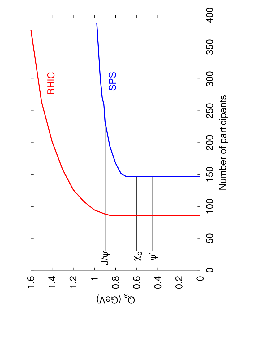
Figure 13: Left: Centrality dependence of the percolation scale Q_S where charmonium suppression is thought to set in for RHIC energy and SPS energy [DFP02]. Right: The ratio of the measured and expected J/$\psi$ yield showing a step like suppression pattern as the number of participants in the collisions system increases [Sat03].

Other important observations made in heavy-ion collisions include the suppression of J$/\psi$ production, strangeness enhancement, the coincidence of particle ratios with statistical model predictions, the enhancement of baryon production, and the reduction of the net baryon number. Figure 13 (right) shows the ratio of the expected and measured J$/\psi$ yields versus N_part. The step like behavior was interpreted as being caused by the dissolution of successive charmonium states in a new form of matter created in heavy-ion collisions. First the $\psi^{\prime}$ and $\chi_{C}$ dissolve and then the J$/\psi$ dissolves. Figure 13 (left) shows the percolation scale where the dissolution of different charmonium states should set in versus N_part [DFP02]. Figure 14 shows the enhancement of the (anti-)proton to pion ratio at intermediate $p_{T}$ in central Au+Au collisions relative to $e^{+}+e^{-}$, p+p, or peripheral Au+Au collisions. The enhancement of baryon production will be studied further in this thesis. Figure 15 shows the enhancement of strange particle production in heavy-ion collisions relative to p+Be collisions. The enhancement increases with the strange quark content; i.e. $\Omega^{-}$(sss) $>\Xi^{-}$(dss) $>\Lambda$(uds) [Fan02].

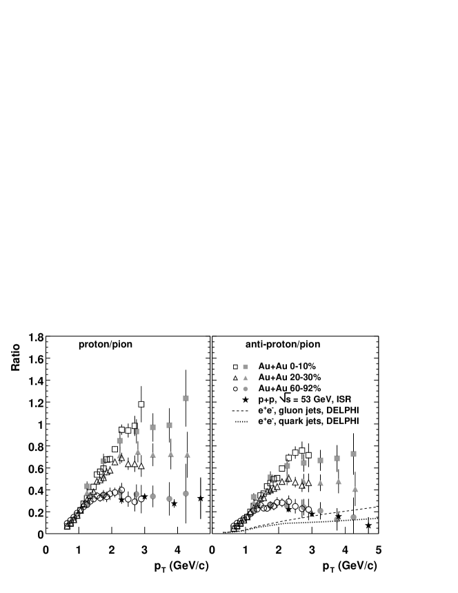
Figure 14: The proton/pion and anti-proton/pion ratio [Adl03e].

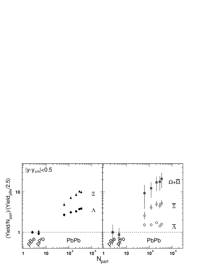
Figure 15: Strange particle yields scaled by $\mathrm{N_{part}}$ normalized by p-Be collisions [Fan02].

5 Thesis Outline

In this thesis, we present the first measurement of $R_{CP}$ for $K_{S}^{0}$ and $\Lambda+\overline{\Lambda}$ for Au+Au collisions at $\sqrt{s_{{}_{NN}}}=200$ GeV and the first measurements of $v_{2}$ for $K_{S}^{0}$ and $\Lambda+\overline{\Lambda}$ for Au+Au collisions at $\sqrt{s_{{}_{NN}}}=130$ and 200 GeV. Our emphasis is on probing the early stage of heavy-ion collisions, mapping out the transition between $p_{T}$ regions (i.e. soft, intermediate, hard, etc.), and understanding how hadronization modifies the observables we measure. In mapping out the $p_{T}$ regions we hope to learn what processes dominate particle production within each region. Studying the variation in yields with centrality ($R_{CP}$) and azimuthal angle ($v_{2}$) for different particle species will help us understand the hadronization mechanisms in heavy-ion collisions. This information will be helpful for characterizing the matter created in heavy-ion collisions.

In Chapter 2 we will discuss the facilities used to study heavy-ion collisions. The Relativistic Heavy-Ion Collider (RHIC) will be described, an introduction to particle tracking detectors will be given, and the Solenoidal Tracker at RHIC (STAR) detector system will be reviewed. Chapter 3 contains details of the analysis methods. In Chapter 4 we present the results of the analysis and in Chapter 5 we discuss these results, draw conclusions, and present an outlook for future work. In the appendices we include a description of the coordinates system in the transverse plane, calculations of the nuclear overlap density for Au+Au collisions, definitions for the kinematic variables used in this thesis and a list of STAR collaborators and institutions.

Chapter 1 Experimental Set-up

1 The Relativistic Heavy-Ion Collider

The Relativistic Heavy-Ion collider (RHIC) at Brookhaven National Lab (BNL) is designed to collide counter-rotating heavy-ion beans at energies up to 100 GeV/u. RHIC is the first facility to collide heavy-ion beams. The center-of-mass energy for these collisions is roughly a factor of ten times greater than the highest energies reached with the previous fixed target heavy-ion experiments. Parameters for existing and future relativistic heavy-ion facilities are given in Table 1. RHIC consists of two concentric rings of super-conducting magnets (cooled to below 4.6 degrees Kelvin) that focus and guide the beams and a radio frequency ($rf$) system that captures, accelerates and stores the beams. The ring’s diameters are approximately 1.22 km.

	AGS	AGS	SPS	SPS	SPS	RHIC	RHIC	LHC
Start year	1986	1992	1986	1994	1999	2000	2001	2006
Amax	28Si	197Au	32S	208Pb	208Pb	197Au	197Au	208Pb
E${}_{P}^{max}$ [AGev]	14.6	11	200	158	40	$0.91$E$4$	$2.1$E$4$	$1.9$E$7$
$\sqrt{s_{{}_{NN}}}$ [GeV]	5.4	4.7	19.2	17.2	8.75	130	200	6000
$\sqrt{s_{{}_{AA}}}$ [GeV]	151	934	614	$3.6$E$3$	$1.8$E$3$	$2.6$E$4$	$4$E$4$	$1.2$E$6$
$\Delta y/2$	1.72	1.58	2.96	2.91	2.22	4.94	5.37	8.77

Table 1: RHIC compared to existing and future facilities; A_max is the maximum species mass number, E${}_{P}^{max}$ is the maximum (equivalent) fixed-target beam energy per nucleon, $\sqrt{s_{{}_{NN}}}$ is the maximum center of mass energy per nucleon, $\sqrt{s_{{}_{AA}}}$ is the total center of mass energy, and $\Delta y/2$ is the rapidity gap from the beam to mid-rapidity [LR02].

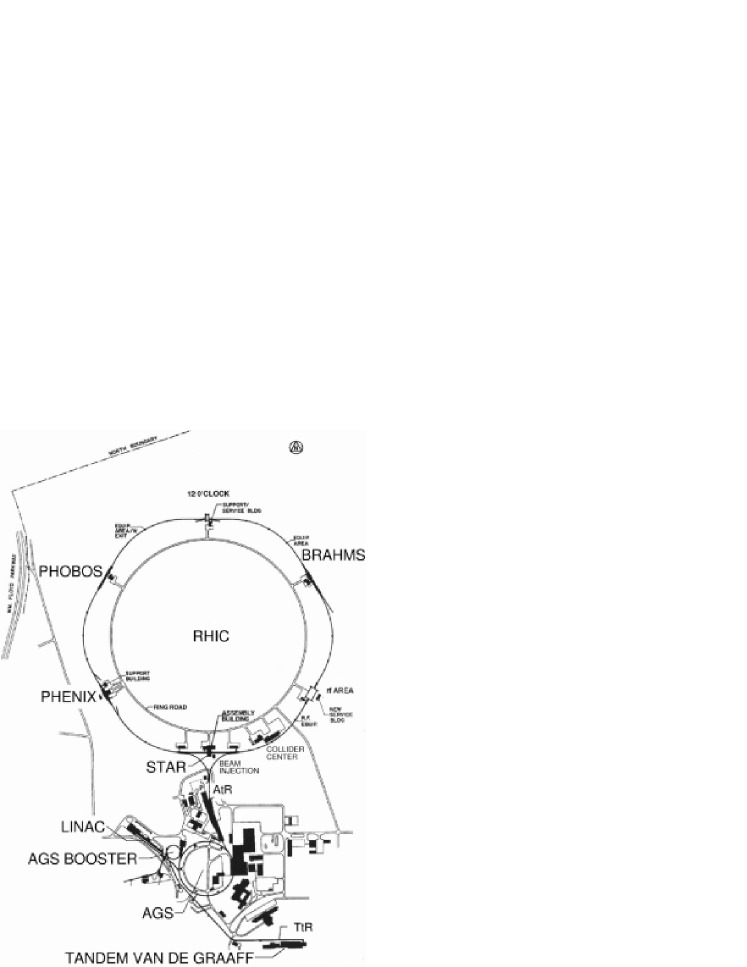
Figure 1: A diagram of the Brookhaven National Laboratory collider complex including the accelerators that bring the nuclear ions up to RHIC injection energy (10.8 GeV/u for ¹⁹⁷Au⁷⁹).

Figure 1 shows the BNL accelerator complex including the accelerators used to bring the gold ions up to RHIC injection energy. In the first of the Tandem Van de Graaff accelerators, gold ions in a charge state $Q=-1e$ accelerate to 15 MeV. The ions then pass through a stripping foil (located between the Van de Graaffs) where electrons are knocked off so that their most probable charge state becomes $Q=+12e$. With their charge changed from negative to positive, the ions gain another 1 MeV/u of energy as they accelerate through the second Van de Graff, back to ground potential. On exiting the Tandem, the ions pass through a second stripping foil bringing their most probable charge to $Q=+32e$. They are then injected into the Booster synchrotron and accelerated to 95 MeV/u. A stripper foil in the transfer line between the booster and the Alternating Gradient synchrotron (AGS) increases their charge state to $Q=+77e$. In the AGS the ions are accelerated to 10.8 GeV/u. They are extracted from the AGS and passed through one final stripper foil where the remaining K-shell electrons are removed ($Q=+79e$). Finally, they are injected into RHIC where they are accelerated to top energy and can be stored for up to 10 hours. Table 2 lists important parameters for RHIC.

Top Au+Au $\sqrt{s_{{}_{NN}}}$	200 GeV
Ave. luminosity $\mathcal{L}$ (10 hour store)	$\sim 2\times 10^{26}$ cm-2s-1
Bunches per ring	60
Gold ions per bunch	$10^{9}$
Crossing points	6
Beam lifetime (store length)	$\sim 10$ hours
RHIC circumference	3833.845 m

Table 2: Nominal RHIC parameters for Au+Au collisions.

2 RHIC Experimental Program

To date, RHIC has generated collisions between gold nuclei at $\sqrt{s_{{}_{NN}}}=$ 22, 56, 130, and 200 GeV, between protons at $\sqrt{s_{{}_{NN}}}=200$ GeV, and between gold and deuterium nuclei at $\sqrt{s_{{}_{NN}}}=200$ GeV. Table 3 shows the luminosity achieved at the end of RHIC Run-2 (Au+Au collisions at $\sqrt{s_{{}_{NN}}}=200$ GeV). The STAR experiment recorded integrated luminosities $\mathcal{L}\sim 2.8\>b^{-1}$ and $\mathcal{L}\sim 80\>\mu b^{-1}$ for RHIC Run-1 (Au+Au collisions at $\sqrt{s_{{}_{NN}}}=130$ GeV) and RHIC Run-2 respectively. Most of the integrated luminosity comes late in the runs, after the collider is tuned.

Bunches	Ions/Bunch	$\mathcal{L}_{peak}$	$\mathcal{L}_{ave}$ (store)	Integrated
		[cm-2s-1]	[cm-2s-1]	$\mathcal{L}$ [($\mu$b)-1]
55	$6\times 10^{8}$	$3.7\times 10^{26}$	$3.7\times 10^{26}$	$\sim 80$

Table 3: The performance of RHIC during the 2001 Au+Au run (Run-2).

There are four experimental collaborations at RHIC; the PHOBOS collaboration with 107 members from 8 institutions, the BRAHMS collaboration with 51 members from 14 institutions, the PHENIX collaboration with 328 members from 52 institutions, and the STAR collaboration with 293 members from 39 institutions .

PHENIX event display	STAR event display
Two muon spectrometers cover the pseudo-rapidity region $1.1<|\eta|<2.4$ and azimuth angle $0<\phi<2\pi$. A central spectrometer with two arms and tracking sub-systems (each subtending $\pi/2$ radians) covers $|\eta|<0.35$. With a smaller acceptance and faster detectors the emphasis is on triggering on rarer probes, hadron identification and electron identification.	A large acceptance solenoidal tracking detector with particle identification covers the full azimuth ($|\phi|<\pi$), $|\eta|<2.0$ and $2.5<|\eta|<4.0$. Subsystems include a central TPC, two forward TPCs, a silicon vertex tracker and a barrel electromagnetic calorimeter. The emphasis is on global event characterization, resonance identification, fluctuations and event-by-event variables.
PHOBOS event display	BRAHMS detector
Measurements of charged particles are made across a full solid-angle with a multiplicity detector. Two small acceptance spectrometer arms allow for particle identification at mid-rapidity. Multiplicity measurements across a broad range of $\eta$ and $p_{T}$ are emphasized.	Designed to provide good particle identification across a broad rapidity and $p_{T}$ range ($0<y<4$; $0.2<p_{T}<3.0$ GeV/c) with two small solid-angle spectrometers. Measuring particle production at forward angles is emphasized.

Table 4: Summary of RHIC experiments.

In this thesis we present an analysis of Au+Au collisions recorded by the STAR detector during the summer of 2000 and the winter of 2001. Approximately $5\times 10^{5}$ and $5\times 10^{6}$ usable events were recorded at $\sqrt{s_{{}_{NN}}}=130$ GeV and $\sqrt{s_{{}_{NN}}}=200$ GeV respectively.

3 Particle Tracking Detectors

The primary detector used for the analysis presented in this thesis is the STAR Time Projection Chamber (TPC). The TPC is designed to do particle tracking which facilitates the identification of secondary vertices from weak decays (e.g. $K^{0}_{S}\rightarrow\pi^{+}+\pi^{-}$). In the following we give an introduction to high-energy particle tracking technology [SKN03].

1 History of Particle Tracking

Since the beginning of particle physics, when J.J. Thomson realized that the cathode rays he was studying were not “rays” but streams of subatomic charged particles instead, our understanding of the subatomic realm and the mechanics that governs it has depended strongly on our ability to detect the tracks of charged particles. Thomson was able to surmise the existence of electrons, measure their charge to mass ratio and even measure their velocity as they were emitted by a hot filament because he could see their trajectory as they passed through crossed electric and magnetic fields. During the years since Thomson’s experiments in 1897 many techniques have been developed to detect or visualize charged particle tracks—nuclear emulsions, cloud chambers, bubble chambers, spark chambers, streamer chambers, other gas detectors, solid-state detectors and so on. All of these techniques rely on very fast charged particles ionizing atoms as they pass through matter. The ionization left along the paths of the high-energy particles can then act as catalysts for reactions that leave an observable trace—such as, a bubble, a spark, condensation, or a charge cascade.

Many of these particle detecting techniques have—because of their inherent limitations—been abandoned for the most part in favor of gas or solid state detectors. Experiments at the newest colliders like RHIC or the LHC rely almost exclusively on these two techniques because they lend themselves well to triggering, high event rates and the digitization of huge amounts of data. Bubble chambers however, are of particular historic importance and produced a wealth of information from their inception in 1952 to well into the 1970s. Their importance to high-energy physics was acknowledged with a Nobel prize in 1960 awarded to Donald Glaser. Glaser struck upon the idea of a bubble chamber when he saw the tracks created by bubbles in beer.

2 Bubble Chambers—Three Decades of Physics and Two Nobel Prizes

Bubble chambers initially used liquid in a super-heated state to detect the ionization left along the tracks of high-energy charged particles passing through the liquid. In 1952 Glaser used diethyl-ether heated to $\sim 100^{\circ}$C above its boiling point to build the first bubble chamber. The super-heated liquid, when struck by cosmic rays, began boiling violently and a photograph made using a fast camera showed tracks left behind by the high-energy charged particles created by a cosmic ray. It is presumed that after a high-energy particle causes the initial ionization along its path, heat generated by recombination is responsible for the boiling and bubble formation in the liquid.

Improvements to this technique, including the use of pistons to create a sudden pressure drop to induce bubble formation, led to greater precision and larger chambers that could be placed in a magnetic field. Perhaps the most notable improvement to the bubble chamber came when Luis Alvarez substituted hydrogen for the ether used by Glaser. Alvarez’s chamber produced much clearer tracks and this technological advance was of such value that he won the Nobel prize for physics in 1968 for his work, the second Nobel prize awarded for work related to the development of the bubble chamber.

In bubble chambers, the fluids in the chamber act both as the target and as the detector so different fluids—some cryogenic and some room temperature—were eventually used to suit the purpose of the experiment. Cryogenic liquids consisted of the simplest nuclei like, H₂, D₂, He, Ne, Ar and Xe while the room temperature “heavy liquids” like propane (C₃H₈) and Freon (CF₂Cl₂ or CF₃Br) offered short interaction lengths. The typical size of a bubble in a bubble chamber is $\sim$ 10 $\mu$m and the bubble density can be used to determine $\beta\equiv v/c$ for the passing particle.

The advantages bubble chambers offered kept them in widespread use for three decades, from the 1950’s to well into the 1970’s. They had good spatial resolution (10 – 150 $\mu$m), a large sensitive volume, $4\pi$ geometrical acceptance; and they permitted the use of a variety of materials as targets. Eventually however, as physics began requiring more complex triggers and as large-volume high-precision detectors demanding electronic data recording came in use, the bubble chambers disadvantages rendered them obsolete. The analysis of photographs was a tedious task requiring expensive projectors for scanning the images and the whole process was only modestly scalable so that only limited statistics could be achieved. Bubble chambers were also complicated to operate, required cryogenics, and were a safety concern. In addition, bubble chambers weren’t compatible with particle colliders—the now dominant high-energy accelerator, they provided no triggering for low cross-sections and they had a relatively long sensitive time ($\sim$ 1 ms) which necessitates a lower beam luminosity.

3 Streamer chambers—a Precursor to Modern Gas Detectors

The streamer chamber developed by G.E. Chikovani in 1963—an improvement on the spark chamber—overcame some of the limitations of the bubble chamber and was the predecessor of the gaseous detectors of today. Like the bubble chamber however, the streamer chamber also relied on photographic film to record the tracks of streamers, placing a limit on the statistics available for analysis.

The spark chamber uses a large potential across two parallel planes of electrodes to induce electrical breakdown—a spark—in gas between the electrodes. The ionization left from the passing of a high-energy particle acts as the catalyst for the spark. The spark chamber however, can only measure the position of the track in the direction parallel to the electric field to within the spacing of the electrodes. The streamer chamber overcomes this limitation by applying a high-voltage pulse for a short duration ($\sim$ 15 ns). The strong electric field ($\sim$ 20 kV/cm) from the high-voltage pulse induces an incomplete spark discharge. These electron avalanches or streamers form all along the particles path and the radiation of the gas in the streamer plasma can be recorded optically. Streamer chambers were built with sensitive volumes of several cubic meters that recorded particle tracks in any direction with equal efficiency. The density of the streamers can be used for particle identification up to particle momenta of $\sim$ 1 GeV/c.

The two major advantages of the streamer chamber over the bubble chamber are its ability to be triggered by external devices and its very short sensitive time ($\sim$ 1 $\mu$s). Eventually however, its use of photographic film, its limited spatial resolution ($\geq~{}300~{}\mu$m) and its relatively long dead time ($\sim$ 300 ms) turned out to favor the gaseous detectors that would rely on electronic, not optical, recording techniques.

4 Today’s Tracking Detectors

Almost all tracking detectors, other than the solid state and gaseous detectors using electronic recording techniques have been abandoned. The modern-era detectors have shorter sensitive times and shorter dead times so that the beam intensity of the particle accelerator can be increased and greater statistics can be recorded. These newer detectors also tend to be easier to operate and have greater spatial resolution.

5 Gas Detectors

Most gas detectors—multi-wire proportional chambers (MWPC), drift chambers, straw tubes, cathode strip or pad chambers, time projection chambers (TPC) and micro-strip gas chambers (MSGC)—use the proportional counting mode of operation. In this mode, the electrons from the primary electron-ion pairs created by the high-energy charged particle, are directed in an electrostatic field toward a very high field region (10–100 kV/cm) surrounding an anode wire of small radius. In this region, the fast electrons gain enough energy to create secondary electron-ion pairs. Each new electron produced by ionization, in turn, creates more electrons-ion pairs; the development of this avalanche or cascade is called gas multiplication. Most of the electrons in the avalanche are created very close to the wire so they are collected within a few nanoseconds. The heavier ions—also predominantly produced near the wire—move more slowly across a larger potential difference. As they do so, they induce a signal that can be detected with an amplifier and used for position and energy loss (dE/dx) measurements.

The mode of operation of a gaseous detector is determined by the response of the ions and gas to the field strength surrounding the anode. In the proportional mode of operation the field strength is great enough to induce gas amplification—typically $10^{4}$–$10^{6}$ times—but is not so great that it leads to complete breakdown or non-negligible space charge effects:caused by the build up of longer-lived positive ions. In the proportional mode of operation the signal is proportional to the number of primary electron-ion pairs which is in turn proportional to the energy lost by the traversing particle. The measured dE/dx can then be used for particle identification (PID).

A multi-wire proportional chamber consists of planes of independent wires—typically spaced 1–2 mm apart—set between two planes of cathodes at a distance of 3–4 times the wire spacing. A negative voltage is applied to the cathodes and the wires are held at ground. Each wire then acts as a proportional counter for primary electrons-ion pairs left along a particles track. The distance from cathode to anode is typically about 1 cm and the wire diameter should be about 20–50 $\mu$m. The spatial resolution is given by $d/\sqrt{12}~{}=~{}300-600~{}\mu$m, where d is the wire pitch or spacing. For this invention G. Charpak was awarded the 1992 Nobel prize in physics.

A drift chamber is a multi-wire proportional chamber with a large wire pitch—from several centimeters up to 50 cm but more typically 5 cm. Track position is determined by measuring the time electrons need to reach the anode wires. The speed of the electron drift depends on the gas used and the pressure in the chamber and is typically $\sim$ 5 cm/$\mu$s so that a timing resolution of 1 ns gives a spatial resolution of $\sim$ 50 $\mu$m. Different geometries and configurations can be used in order to create constant fields pointing toward the anode wires. A straw tube is a drift chamber composed of an individual straw shaped cathode (diameter of $\sim$ 5 mm) with a single anode wire in the center. A “continuous” tracker can be constructed by packing many layers of straw tubes together. Straw tube detectors tolerate high loads because they don’t use a common gas volume and can achieve a resolution of about 150 $\mu$m with coarse time measurements.

A time projection chamber (TPC) is a drastic variation on a simple drift chamber. A TPC consist of a large three-dimensional gas filled vessel with readout detectors on a wall at the end of a drift volume. The readout detectors are usually cathode pad chambers. A strong electric field across the TPC produced by a cathode on the wall opposite the readout planes creates the drift field. When a charged particle creates electron-ion pairs within the drift volume the strong drift field prevents them from recombining. The much lighter electrons move quickly toward the readout chambers. The drift field is chosen so that it is not strong enough to create secondary electron-ion pairs: typically hundreds of volts per centimeter. The readout chamber is separated from the drift volume by a gating grid. The gating grid is a plane of wires that electrostatically separates the amplification region from the drift region. The gating grid prevents the ions created in the amplification region from getting back into the drift region and allows for triggering of the detector; when an interesting event occurs the gating grid wires are set to voltages that allow electrons to pass through.

The TPC readout chambers typically consist of an anode wire plane between a ground wire plane and a cathode pad plane. The signal induced on the anode wires is typically detected via image charges on several nearby pads. The position of the electron-ion cascade in the anode wire direction can be determined precisely by fitting a modified Gaussian to the signals on several consecutive pads. This measurement gives two transverse coordinates and the drift time gives the third coordinate, making the TPC a fully three-dimensional detector. Unlike other historic three-dimensional detectors however, such as the bubble or streamer chambers, the TPC is read completely electronically. The TPC also has the advantage that it has no pulsed very high-voltages and is fast compared to historic detectors: its speed is determined by the maximum drift time which, for large chambers is $\sim$ 100 $\mu$s.

Inhomogeneities in the drift field and effects due to magnetic fields however, can distort the drift path of the electrons and further degrade the resolution. The electron clouds also diffuse at a rate of hundreds of $\mu$m/$\sqrt{cm}$ due to elastic rescattering in the gas as they drift toward the readout chamber. The TPC requires careful tuning of the drift field and a high degree of gas purity. Many parameters like drift length, track angle, or the number of primary ions affect the spatial resolution but a typical value is $\sim$ 500 $\mu$m.

6 Solid State Detectors

Solid state detectors—silicon micro-strip detectors, silicon pixel detectors and silicon drift detectors—offer very good resolutions of $\pm$ 10 – 100 $\mu$m and are now in common use. Every detector planned at the Large Hadron Collider at CERN (LHC) will use trackers based on silicon devices. Silicon detectors require only 3.6 eV of energy from the traversing particle to create an electron-hole pair. That is roughly one order-of-magnitude less than gas detectors require ($\sim$ 30 eV). This, along with silicon’s higher density, means that the number of electron-hole pairs created by a minimum ionizing particle (MIP) in silicon is much greater than the number of electron-hole pairs created over the same distance in gas. In 1 $\mu$m of silicon a MIP produces $\sim$ 100 charge pairs. To produce that much charge in gas would require several centimeters. As a result, unlike gaseous detectors, silicon detectors don’t require signal amplification inside the detector; in a typical silicon detector a MIP will produce 20 – 30 thousand electrons.

Typically, silicon detectors are built using $\sim$ 300 $\mu$m thick, high resistivity, n-doped silicon plates with a thin p-doped layer on one side. A reverse bias voltage—positive on the n-side and negative on the p-side—is applied to deplete the silicon of free charge carriers and to create an electric field that will cause the electrons and holes to drift to opposite surfaces where readout structures are organized. The highly developed state of silicon technology allows for the production of many different readout structures.

The readout structures for both silicon strip and silicon pixel detectors are layers of aluminum applied to the surface of the silicon. Silicon strip detectors use a solid layer of aluminum on the n-doped side of the silicon and a sequence of aluminum strips on the p-doped side. The strips typically have a pitch (d) of $\sim$ 50 $\mu$m. The resolution for this pitch is $\sim$ 15 $\mu$m or $d/\sqrt{12}$. The charge collected on the strip is electronically integrated and read out as an analogue or digital signal. If strips are placed on both sides of the silicon—a double sided silicon strip detector—two coordinates can be measured simultaneously.

The silicon pixel detector uses pixels instead of strips and has the advantage that it is a true two dimensional micro-detector. Amplifier circuitry however, needs to be connected to each pixel which typically has a surface area of only $\sim 50\times 400\mu$m². This is done using specially designed readout chips that are bump-bonded to the detector silicon. Silicon pixel detectors are fast, have very low noise (small capacitance) and have excellent pattern recognition for high particle densities. They require however, a large number of readout channels (100 million is not uncommon), are very fragile and offer many technological challenges in development.

Silicon drift detectors have two-dimensional capabilities but by their design avoid the large number of channels required by silicon pixel detectors. Silicon drift detectors use a silicon wafer, with an array of anodes arranged at one edge and cathodes at the other. An electric field drifts the primary electrons—from the track of a passing particle—through the silicon, toward the array of anodes. A typical drift speed is $\sim$ 15 mm/$\mu$s. The anode position along the edge of the wafer and the drift time give two coordinates for the position of the track. The third coordinate is given by the position of the wafer and, like a spark chamber, is only known to within the thickness of the wafer. The signal on the anodes can be read out at $\sim$ 40 MHz—a very high frequency—but the time for the electrons to drift to the anodes ($\sim$ 5 $\mu$s), makes it a relatively slow detector. In addition, these detectors require very precise climate control because of the dependence of the drift time on temperature. The high resolution of all these solid state detectors however, makes them ideal for constructing vertex chambers that are particularly useful for detecting heavy-flavor particles.

4 The STAR Detector System

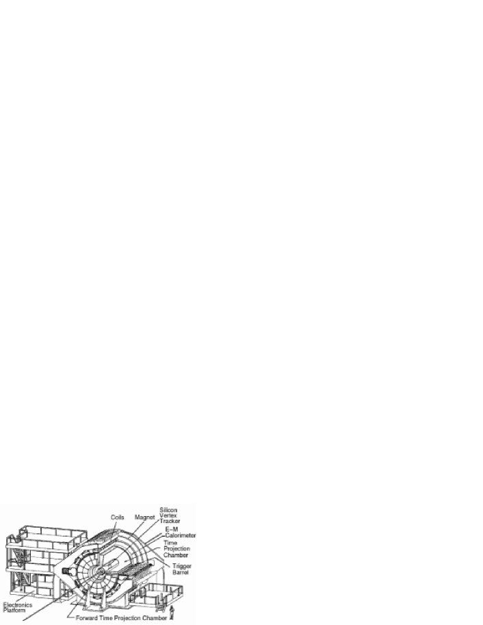
Figure 2: View of the STAR detector system.

The STAR detector [Ack03] (Figure 2) is an azimuthally symmetric, large acceptance, solenoidal detector designed to measure many observables simultaneously. The detector consists of several subsystems and a large Time Projection Chamber (TPC) located in a 0.5 Tesla solenoidal analyzing magnet.

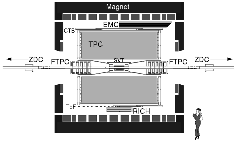
Figure 3: Cutaway of the STAR detector in its 2001 configuration; including a partial installation of the electromagnetic calorimeter (EMC), the temporary ring-imaging Cherenkov detector (RICH), and a time-of-flight detector (ToF) prototype.

The layout of the STAR detector system as it was for Run-2 is shown in Figure 3. The active subsystems included two RHIC-standard zero-degree calorimeters (ZDCs) that detect spectator neutrons, a central trigger barrel (CTB) that measures event multiplicity, a ring-imaging Cherenkov and time-of-flight detector that extend particle identification to higher $p_{T}$, 10 percent of the full barrel electromagnetic calorimeter to measure photons, electrons and the transverse energy of events, and four tracking detectors. The tracking detectors are the main TPC, two forward TPCs, and the silicon vertex tracker (SVT).

The TPC is STAR’s primary detector [And03] and can track up to $\sim 4\times 10^{3}$ particles per event. For collisions in its center, the TPC covers the pseudo-rapidity region $|\eta|<1.8$. It can measure particle $p_{T}$ within the approximate range $0.07<p_{T}<30$ GeV/c. The momentum resolution $\delta p/p$ depends on $\eta$ and $p_{T}$ but for most tracks $\delta p/p\sim 0.02$. The full azimuthal coverage of the STAR detector ($-\pi<\phi<\pi$) makes it ideal for detecting weak decay vertices, reconstructing resonances and measuring $v_{2}$ and other variables requiring event-by-event characterization.

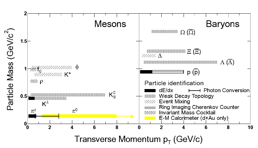
Figure 4: The $p_{T}$ reach of STAR’s particle identification capabilities with the 2001 detector setup.

Figure 4 illustrates the STAR detector’s particle identification capabilities during Run-2. These capabilities will be further enhanced with detector upgrades, larger data samples, and more advanced triggering to select rare events. Most of the measurements illustrated in Figure 4 are limited in $p_{T}$ coverage by the statistics available. Using the topology of their weak decays in the TPC, the $K_{S}^{0}$ and $\Lambda(\overline{\Lambda})$ were identified across the largest $p_{T}$ range ($0.3<p_{T}<7.0$ GeV/c). The kinematic reach of these and other topologically identified particle measurements (i.e. $\Xi(\overline{\Xi})$, and $\Omega(\overline{\Omega})$) will reach their limit when the momentum of the daughter tracks becomes too high to be accurately measured in the TPC. As the momentum resolution worsens the invariant mass calculation will become less accurate. As a result, the width of the mass peak will broaden. In addition, low $p_{T}$ particles mis-measured as high $p_{T}$ particles will start to dominate the less prominent high $p_{T}$ signal (feed-down). The $p_{T}$ scale where the analysis fails has not been extensively studied but should depend on the specific particles decay topology. We naively expect the $K_{S}^{0}$ identification to fail first, around $p_{T}\sim 15$ GeV/c, where the high $p_{T}$ signal will be dominated by low $p_{T}$ feed-down. For comparison, the $\pi^{0}$ identification in the EMC is limited by the detector technology to roughly $1.5<p_{T}<20$ GeV/c.

With detector upgrades and increased data samples, STAR has the potential to measure the yield of heavy-flavor mesons and baryons (particularly for D mesons), charmonium production (J/$\psi$), and direct photon production. Given its extensive array of particle identification and event characterization capabilities, the STAR detector is particularly well suited for characterizing the matter created in heavy ion collisions.

1 The STAR Trigger Detectors

The bunch crossing rate at RHIC is $\sim 10$ MHz while the read-out rate for the STAR TPC is $\sim 100$ Hz. When the interaction rates approach the bunch crossing rates, the STAR trigger must reduce the event rate by five orders of magnitude. The STAR trigger needs to reject background, such as beam-gas interactions (expected rate $\sim 100$ Hz), select events that best further our physics goals, and issue triggers to the other detectors. Furthermore, the future success of STAR may depend on the ability to trigger on rare events.

With recent upgrades, the STAR detector system has four fast detectors that can be used as trigger detectors: the central trigger barrel (CTB), the zero-degree calorimeters (ZDC), a multi-wire counter (MWC), and the barrel electromagnetic calorimeter (EMC). In addition, a beam-beam counter (BBC), a forward $\pi^{0}$ detector (FPD), and an endcap electromagnetic calorimeter (EEMC) will become available for triggering [Bie03].

The CTB measures the charged particle multiplicity. With 240 scintillator slats each covering $\pi$/30 in $\phi$ and 0.5 in $\eta$, the whole CTB covers $-1.0<\eta<1.0$ and $-\pi<\phi<\pi$ at a radius of four meters. Its multiplicity resolution is $\sim 3$% for multiplicities $>1000$.

Each RHIC experiment has two ZDC’s to monitor beam interactions. The ZDC’s detect the neutrons freed from the Au ions when a collision occurs (spectator neutrons). The STAR ZDC’s are located $\pm 18.25$ m from the nominal interaction region and subtend an angle $\theta<0.002$ radians. Each ZDC consists of three modules with a series of tungsten plates and layers of wavelength shifting fibers that route Cherenkov light to a photo-multiplier tube. The timing of the ZDC signals is also used to locate the longitudinal position of the interaction vertex.

Trigger	Conditions
Hadronic Minbias	[ZDCe $\geq 5$ & ZDCw $\geq 5$] & CTB $\geq 15$ mips
Hadronic Central	[ZDCe $\geq 5$ & ZDCw $\geq 5$] & ZDCsum $<85$
	& [Vertex Cut] & CTB $\geq 2000$ mips

Table 5: The two trigger settings used in this thesis from the 2001 Au+Au data taking.

During the 2000 and 2001 Au+Au runs the CTB and ZDC were used to study minimum-bias, peripheral and central Au+Au collisions. Table 5 lists the ZDC and CTB conditions for the two trigger settings used in this analysis; hadronic minimum-bias and hadronic central. Figure 5 illustrates the selection scheme for these triggers in the ZDC verses CTB plane.

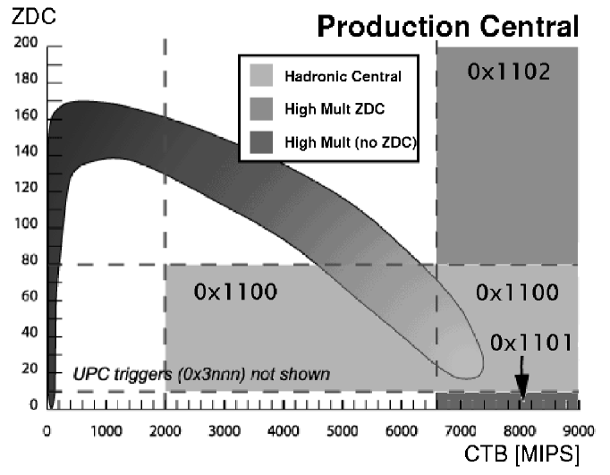
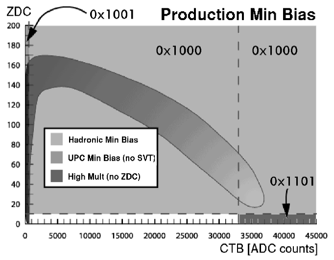
Figure 5: A diagram illustrating the STAR trigger scheme for central (left) and minimum-bias (right) triggers. A central event will have a low ZDC count and a high CTB count.

2 The STAR Time Projection Chamber

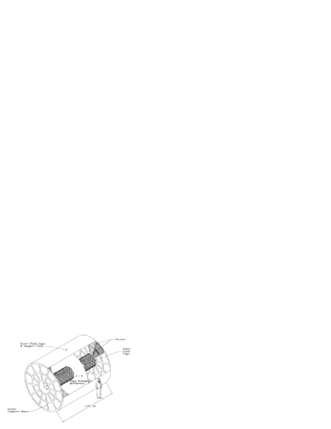
Figure 6: Sectioned view of the STAR TPC showing the inner/outer field cage, the central membrane, and inner/outer sectors.

The STAR TPC (Figure 6) surrounds the beam-beam interaction region. The inner and outer radii of its drift volume are 50 cm and 100 cm respectively. The drift length from the central membrane to either of the ground planes is 209.3 cm. The central membrane is typically held at 28 kV. A chain of 183 resistors and equipotential rings along the inner and outer field cage create a uniform drift field from the central membrane to the ground planes where the anode wires and pad planes are organized into 12 sectors.

Figure 7 shows a cutaway view of the readout pad planes of an outer sub-sector. The first of three wire planes is used as a gating grid. The anode wires are located between a shielding wire plane and the cathode pad plane. In the open configuration the voltage on the gating grid wires is set so that ions pass through freely. When it is closed the field lines terminate on the gating grid wires and the electrons and ions cannot pass. When the TPC is not being read-out the gating grid is closed and prevents ions from drifting back into the TPC drift volume where they can interfere with the uniformity of the drift field.

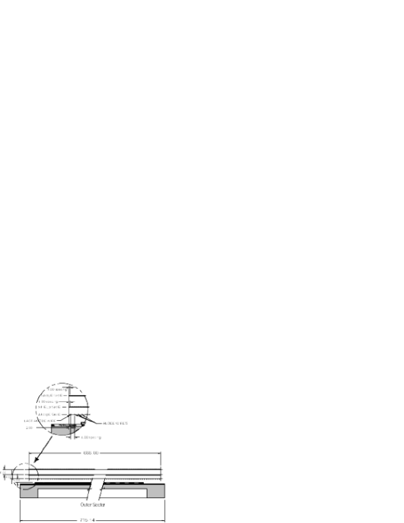
Figure 7: Cutaway of the pad plane of a TPC outer sub-sector.

The second wire plane shields the TPC drift region from the strong fields around the anode wires. As electrons drift past the gating grid and the shield plane they accelerate towards the anode wires and initiate a charge amplifying cascade. The $x$-$y$ position of the electron-ion pair left in the TPC by a high energy particle is determined by the position of the cathode pads that detect the cascade. The $z$ position is determined by the time bucket and the drift velocity. With 136,608 pad planes and 512 time buckets, the TPC has over 70 million three-dimensional pixels. In addition, we use the signal from three adjacent pads to better determine the cluster centroid and so, the resolution in the pad row direction is significantly smaller than the pad size. The resolution depends on the position and orientation of a track relative to the pads, but it is typically 0.5–1.0 mm.

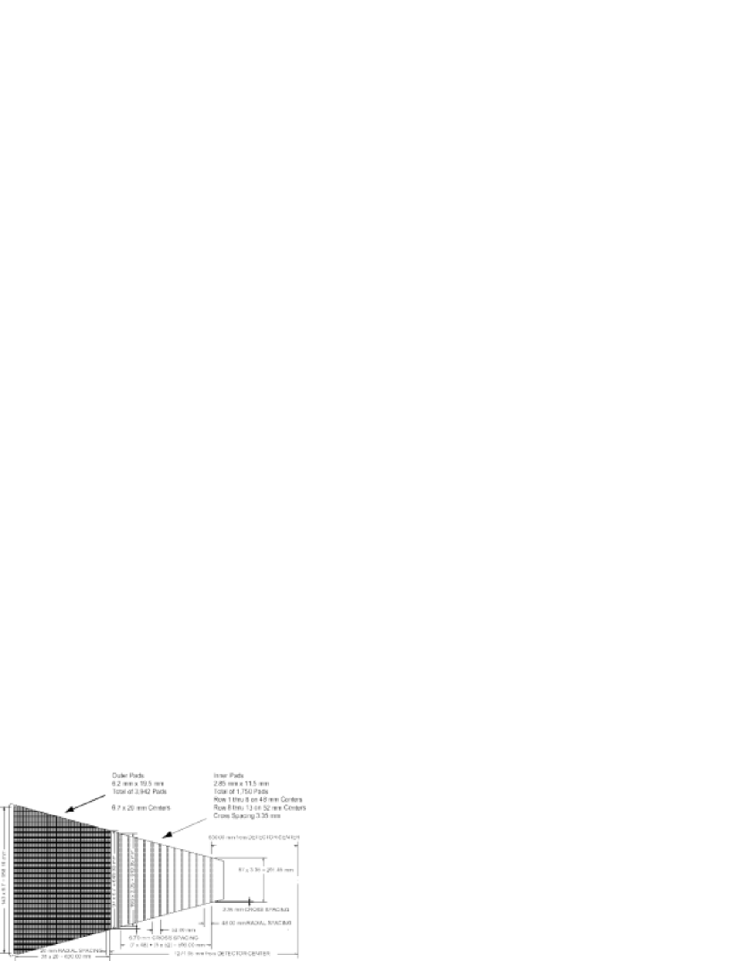
Figure 8: A diagram of a TPC pad plane sector.

Figure 8 shows one sector of the TPC pad plane. The inner sub-sector is designed to handle the higher track density near the collision vertex. Table 6 lists the dimensions of the inner and outer sub-sectors. Because of the size of the front-end electronics, the inner-pad coverage cannot be made continuous.

	Inner Sub-sector	Outer Sub-sector
Pad size (mm)	$2.85\times 11.50$	$6.20\times 19.50$
Pad isolation gap (mm)	0.5	0.5
Pad rows	13	32
Number of pads	1750	3942
Anode to pad spacing (mm)	2.0	4.0
Anode voltage (V)	$1170$	$1390$
Anode gain	$3770$	$1230$

Table 6: Geometry of the inner and outer sub-sectors.

In addition to tracking charged particles, the TPC is also able to identify particles by their mass. High energy charged particles lose energy as they traverse the TPC gas. The average energy loss depends on their velocity, not their momentum $p$. At a given $p$ below 0.8 GeV/c pions, kaons and protons suffer significantly different average energy losses. As such, in this region, measurements of the energy deposited along a particles trajectory can be used to identify the particle. Figure 9 shows the energy loss (dE/dx) measured from tracks in the STAR TPC where the bands correspond to particles with different masses.

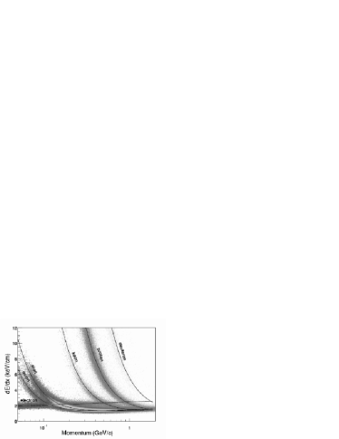
Figure 9: The energy loss of charged particles traversing the TPC gas.

3 STAR TPC Gas System

The TPC gas system [Kot03] supplies the TPC with either one of two gas mixtures—P10 (Ar 90% + CH₄ 10%) while the detector is operating or C₂H₆ 50% + He 50% for purging the TPC when it is not in use. The TPC gas mixture must satisfy multiple requirements. It is the medium where the particles being tracked induce ionization, the medium those electron-ion pairs drift through, and the medium where the electron multiplication takes place. The convenience and safety of the gas is also considered.

Drift Characteristics
Drift Velocity (Maximum)	5.45 cm/$\mu$s	at 130 V/cm
Longitudinal Diffusion	320 $\mu$m/$sqrt(cm)$	0.5 Tesla Field
Transverse Diffusion	185 $\mu$m/$sqrt(cm)$	0.5 Tesla Field
Ionization Characteristics
Charge Created	227 electrons	from a 5.9 keV X-ray (Fe55)
Gain (N/N0) Characteristics
Inner Sector Gain	$\approx 3770$	for V${}_{anode}=1170$ V
Outer Sector Gain	$\approx 1230$	for V${}_{anode}=1390$ V

Table 7: Characteristics of the TPC gas mixture, P10.

The electron drift velocity in P10 is relatively fast and it peaks and saturates at a relatively low electric field (130 V/cm). Operating with a drift field in the saturated region minimizes variations in the drift velocity. Some of the important characteristics of P10 are listed in table 7.

The drift velocity and the gas gain are both sensitive to the pressure and purity of the gas. The TPC gas pressure varies with atmospheric pressure so both of these are monitored. Ionization induced by lasers at fixed locations in the TPC are used to measure the drift velocity. The gas gain is monitored by a gain chamber and by observing the energy loss of tracks in the TPC. Table 8 lists characteristics of the TPC gas system.

System Characteristics
TPC Volume	$50000$ liters
Internal TPC Pressure	$2.0\pm 0.03$ mbar
Recirculation Flow	$36000$ liters/hour
Oxygen Content	$<25$ ppm
Water Content	$<20$ ppm

Table 8: Gas system parameters.

4 TPC Gas Gain Monitor

The UCLA nuclear physics group has been responsible for the construction and installation of a chamber designed to keep a minute-by-minute record of the gain of the STAR TPC gas. At present, we base our corrections for changes in the gas gain—thought to be primarily due to variation in the gas pressure—on measurements of the TPC gas pressure. An attempt is also made to correct for residual variations in the gain by estimating the ionization energy loss in the TPC gas (dE/dx) for tracks which qualify as proton candidates. This step requires averaging together data taken over several hours. The final adjusted gain is then used to make a better measurement of the dE/dx of tracks as they traverse the TPC. As described in Section 2, this critical measurement is correlated with a particles momentum to provide a means of particle identification (PID).

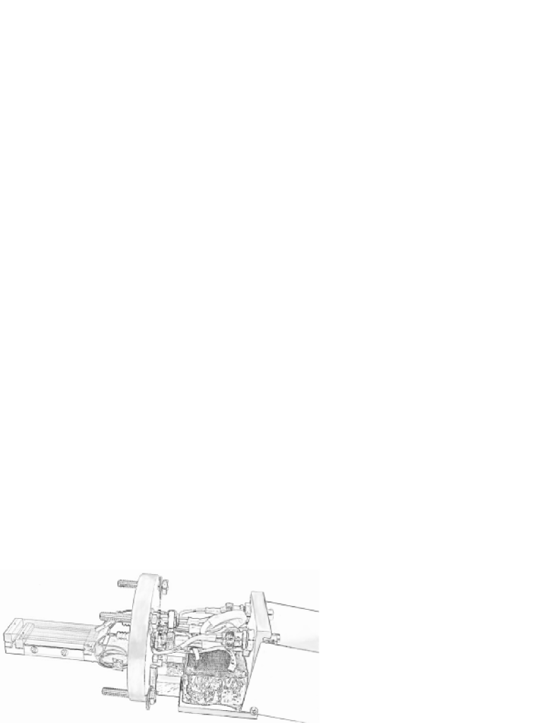
Figure 10: The gain monitor chamber with the wire planes and the shielded electronics exposed. The shielding for the wire planes and the Fe⁵⁵ source are not shown. The aluminum outer housing is folded back and locked into place when the chamber is in use so that the high-voltage wires are not exposed.

With the construction and installation of the new gain monitor chamber complete, we are able to measure the TPC gas gain directly and as such may be able to improve the measurement of dE/dx and PID at STAR. A source of radiation with a known energy is used to ionize the TPC gas flowing through the chamber. The deposited charge accelerates toward the chamber’s high voltage anode wires and a charge amplifying cascade ensues. The pulse generated by the cascade depends on the energy of the incident radiation and the gas gain. We use an Fe⁵⁵ source emitting 5.9 keV photons. The signal from the anode wires is amplified and conditioned with an Amptek A225 pre-amplifier and shaping amplifier and an Amptek A206 voltage amplifier and low-level discriminator. The magnitudes of these pulses are analyzed with an Amptek (PMCA600A) multi-channel analyzer (MCA).

We fit the spectrum of pulse heights from the MCA to an exponential function for the background noise and two Gaussian functions; one for the 5.9 keV peak and another for the secondary photon escape peak at 2.7 keV. The variation in the position of the primary peak is used to monitor the relative magnitude of the gas gain. We are able to keep the noise level low in the spectrum and have found that the resolution of the Gaussian peak is approximately 13%.

The MCA is read and controlled by a PC (BEATRICE.STAR.BNL.GOV) located in the data acquisition (DAQ) room of the STAR hall. No wires can connect the ‘outside world’ to the electronics platform where the MCA is located or to the detector where the chamber is located. Instead, the PC controls the MCA via optical fibers and a SITECH 2506 fiber-optic modem. The chamber is attached to a pipe flange on one of four exhaust manifolds on the face of the TPC. Its wire planes extend into the pipe where the P-10 exhaust flows from the TPC. The chamber (shown in Figure 10) is built to replicate the behavior of the TPC pad planes. Its geometry—including the diameter of the wire used—matches the geometry of the outer sub-sector pads in the TPC. The chamber is electrically isolated from the pipe and the wire planes are shielded from stray fields by a wire mesh cage surrounding them. The Fe⁵⁵ source is mounted inside the wire mesh cage several centimeters above the wire planes. When in operation the anode wire plane is held at +1390 V. The anode plane is located between a grounded pad plane and a wire ground plane. The chambers face is constructed out of non-conducting material so that the bolts used to attach the chamber to the exhaust manifold are isolated from the rest of the chamber. This is necessary because the exhaust manifold does not share the same ground as the TPC and the monitor chamber.

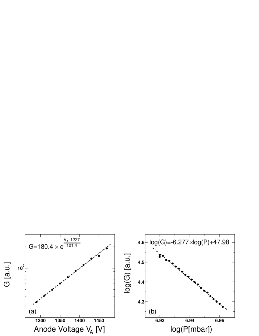
Figure 11: Left: Gas gain versus anode wire voltage. Right: Pressure dependence of the gas gain in P10.

The chamber was tested at UCLA before installation. The gas gain variation with respect to the anode wire voltage is shown in Figure 11 (a). Although we do not anticipate that the gain monitor will ever be used with any voltage other than +1390 V, we ran this test to compare to other gain monitors and to understand how variations in the supply voltage could affect the measured gain. Figure 11 (b) shows the dependence of the gas gain on the gas pressure. The expected relationship of gain to pressure is given by:

$$\frac{dG}{G} \approx-A\frac{dP}{P},$$ (1)

$$\log(G) \approx-A\log(P)+B,$$ (2)

where $G$ and $P$ are the gain and pressure respectively. The coefficient $A$ is expected to be 6.7 $\pm 1.5$ [BR94] and $B$ is an arbitrary constant. In our calibrations we find $A=6.277\pm 0.003$ where the error is statistical only.

The gain monitor recorded data during the entire 2001–2002 data taking. The software proved to be very robust and required little or no maintenance or intervention from the detector operators or shift crew. Several troubling features in the data however, became apparent during the data taking. It was noted early in the Run-2 that the gain measurement varied systematically with the magnetic field setting (shown in Figure 12). Possible causes include variations in the response of the electronics with the magnetic field setting, a change in the charge amplification caused by the orientation of the wire planes relative to the magnetic field, or gas leaks exacerbated by the magnetic field. For the 2003 d+Au collisions the gain monitor was realigned to match the orientation of the TPC pad planes.

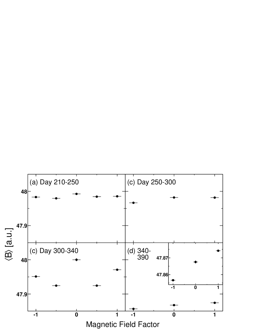
Figure 12: The variation of the gain with the magnetic field—after accounting for the pressure dependence—is shown for four different time periods. The dependence is not strong in the upper-left plot (earlier in the Au+Au Run-2) but subsequent measurements show a strong field dependence. In the inset of panel (d) the vertical axis is adjusted to emphasize the field dependence.

We also find that the relative magnitude of the gas gain decreased with time; as seen in Figure 13 (b). This time dependence was observed in other calibration data and has been accounted for in the dE/dx calibrations. The importance of the gain monitor chamber however, can be seen in Figure 13 (a). Scatter is seen in the plot of $\log(G)$ versus $\log(P)$. This may indicate that there are still variations in the gain not taken into account with the current calibration method—a method that is insensitive to gain variations on a short time scale.

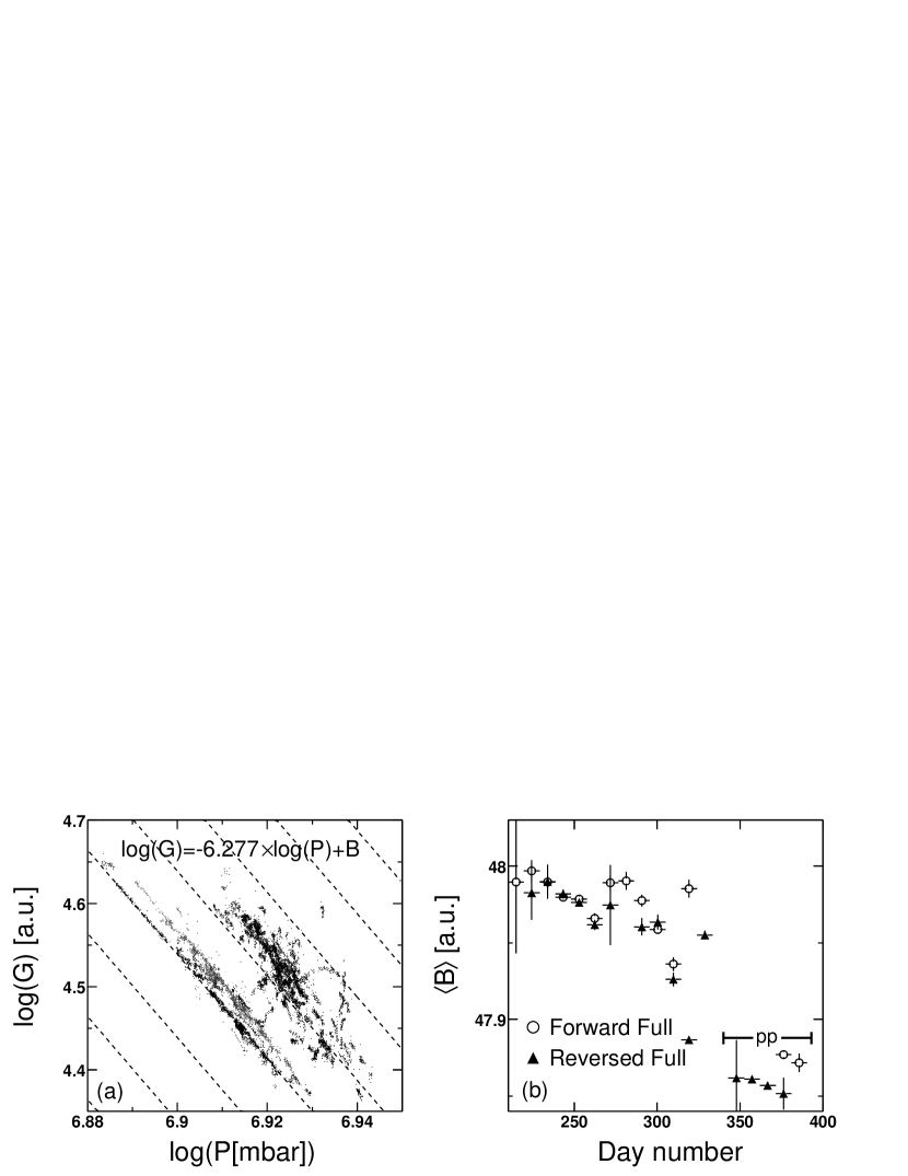
Figure 13: Left: Scatter plot of $\log(G)$ versus $\log(P)$. The contours represent the expected behavior for $\log(G)=-6.277\log(P)+B$. Right: Variation in gain with time: the mean value of the “constant” $B$ is shown after the expected pressure dependence has been parameterized.

Further study of the gain monitor and the gain monitor data is needed before we use it for calibrations. The electronics were returned to UCLA where they were tested in a 0.3 Tesla magnetic field for variations in pulse height with field direction. No effect was observed. We have also built and installed an adapter that rotates the gain monitor so that the wire planes are perpendicular to the magnetic field. In the 2001–2002 data taking the gain monitor data was recorded in the online database, but was not propagated to the off-line database where it can be easily used for calibrations. This will be changed for future data taking and we anticipate that the gain monitor will be used for calibrations as well as diagnostics.

Chapter 2 Analysis Methods

The technique for finding $K_{S}^{0}$, $\Lambda$, or $\overline{\Lambda}$ candidates with the STAR detector and calculating their $p_{T}$ and $y$ distributions is well established [Adl02e, Lon02]. Up to now, measurements of identified particle $v_{2}$ have relied on pure particle identification (90% purity) via dE/dx measurements in the TPC gas [Adl01]. We’ve adapted the $v_{2}$ analysis method to calculate $v_{2}$ for particles identified only on a statistical basis. With this method it is possible to calculate $v_{2}$ for identified particles independent of the particle sample’s signal-to-background ratio.

In this chapter, we describe the selection criteria for events, tracks and the $K_{S}^{0}$, $\Lambda$, or $\overline{\Lambda}$ candidates. Details of the $R_{CP}$ and spectra measurements—including an analysis of systematic errors—are given. Finally, the analysis methods for measuring $v_{2}$ of $K_{S}^{0}$, $\Lambda$, and $\overline{\Lambda}$ are presented along with a discussion of the systematic errors associated with the $v_{2}$ analysis.

1 Event and Track Selection

Data set	Minimum-bias		Central
	Recorded	Used	Recorded	Used
Run-1 ($\sqrt{s_{{}_{NN}}}=130$ GeV)	$0.8\times 10^{6}$	$0.20\times 10^{6}$	$0.8\times 10^{6}$	$0.18\times 10^{6}$
Run-2 ($\sqrt{s_{{}_{NN}}}=200$ GeV)	$4.0\times 10^{6}$	$1.6\times 10^{6}$	$3.5\times 10^{6}$	$1.5\times 10^{6}$

Table 1: The number of Au+Au events used in our analysis.

To date, for the STAR experiment, the number of events that are useful for our analysis has been $\sim 40\%$ of the total recorded. Table 1 lists the number of events recorded and used for Run-1 and Run-2. Events for which no primary vertex is found are discarded. For Run-1, events with $z$-vertex further than 75 cm from the TPC center were discarded. For Run-2, improvements in the accelerator allowed STAR to select only collisions within 25 cm of the TPC center. Still more events are discarded to remove trigger biases. A large sample of minimum-bias data was taken with a tight $z$-vertex cut applied in the level zero trigger that biased the sample. These events require more careful analysis and are not included in this analysis.

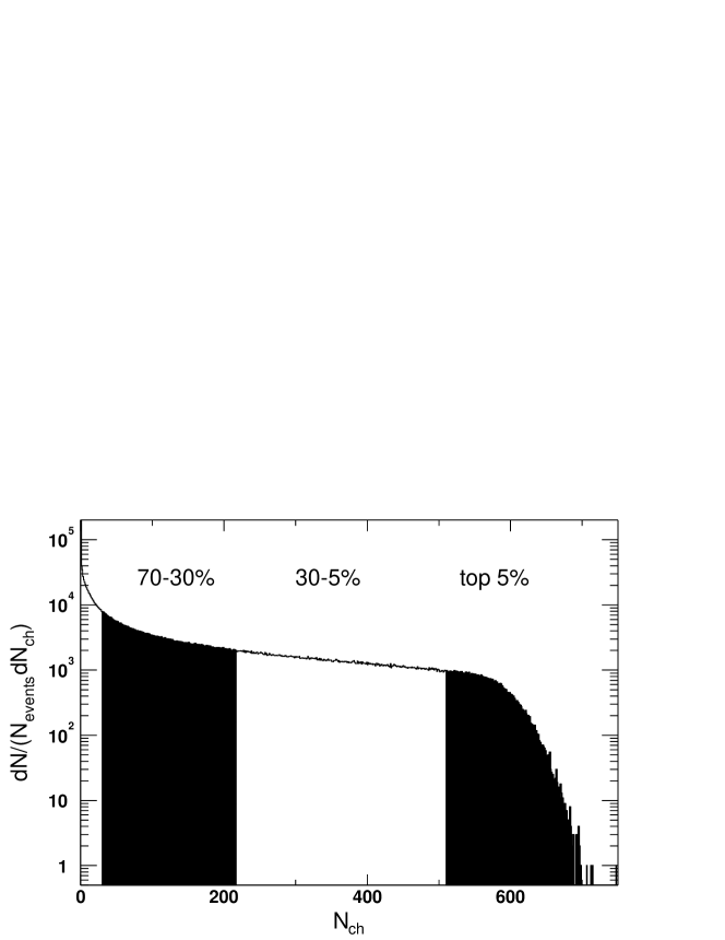
Figure 1: The TPC charged particle multiplicity distribution for $\sqrt{s_{{}_{NN}}}=200$ GeV. N_ch is the number of primary tracks in $|\eta|<0.5$. The fractions of the total cross-section used for the analysis of $v_{2}$ are shown.

The multiplicity as measured by the TPC—not the CTB—is used to define STAR’s centrality intervals. The TPC reference multiplicity for Run-2 is the total number of primary tracks in the TPC with 10 or more fit points, having $|\eta|<0.5$, and a distance of closest approach (DCA) to the primary vertex less than 3 cm. A primary track is defined by a helix fit to the TPC points and to the primary vertex; the global track fits do not include the primary vertex. For Run-1 primary tracks within $|\eta|<0.75$ were used to define the multiplicity.

	Event plane	$K_{S}^{0}$ and $\Lambda(\overline{\Lambda})$
Track set	Primary	Global
DCA to primary vertex (cm)	$<3$	na
Number of hits	$>15$	$>15$
Number of hits/possible hits	$>0.52$	na
$|\eta|$	$<1.5$	na
Momentum (GeV/c)	$0.1<p_{T}<2.0$	$p_{T}>0.05$

Table 2: Track selection criteria for Au+Au collisions at $\sqrt{s_{{}_{NN}}}=200$ GeV.

Table 2 list the selection criteria for tracks used in the analysis of $\sqrt{s_{{}_{NN}}}=200$ GeV data. For the $K_{S}^{0}$, $\Lambda$, or $\overline{\Lambda}$ reconstruction when the dE/dx of a track can be used to identify the particle type, an additional dE/dx cut is made. For $0.2<p_{T}<2.0$ GeV/c, pion candidates are required to have a dE/dx value within $6<\sigma_{\pi}<5$ and proton candidates are required to have a dE/dx value within $2.85<\sigma_{p}<10$. These cuts are very loose and only act to exclude tracks which are obviously not of the correct type. The most effective selection criteria in the identification of $K_{S}^{0}$, $\Lambda$, or $\overline{\Lambda}$ particles are the decay topology cuts.

2 Decay Vertex Topology: Yield Measurements

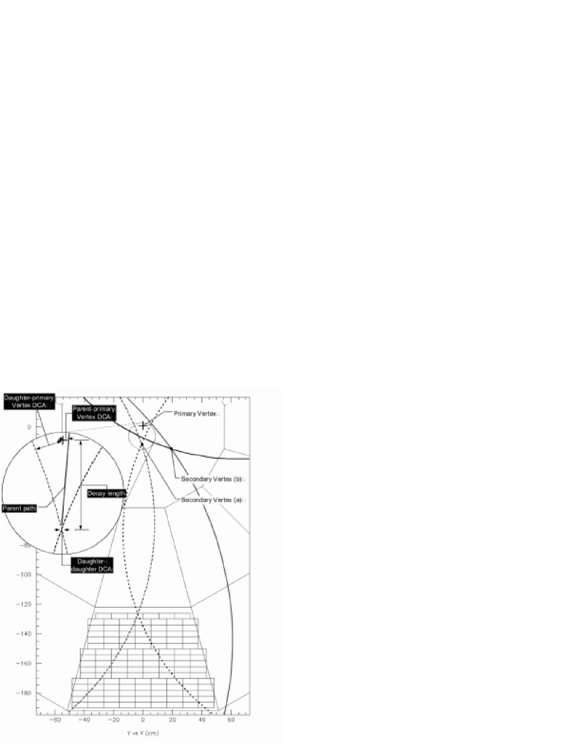
Figure 2: A sketch of the geometry of a neutral particle decay in the TPC. Case ”a” shows charged daughter tracks curving towards each other after they are created in the decay while in case ”b” they are curving away from each other.

We identify the $K_{S}^{0}$, $\Lambda$ and $\overline{\Lambda}$ candidates from the charged daughter tracks produced in the weak decays: $K_{S}^{0}\rightarrow\pi^{+}\pi^{-}$, $\Lambda\rightarrow p\pi^{-}$ and $\overline{\Lambda}\rightarrow\overline{p}\pi^{+}$. To select the $K_{S}^{0}$, $\Lambda$, or $\overline{\Lambda}$ candidates, we calculate the distance of closest approach (DCA) between all combinations of selected global tracks within an event. We define the four-momenta of the daughter particles by assuming they originated from the points on the two helices where the DCA occurs, and by choosing a mass hypothesis appropriate for the weak-decay channel. We use the four-momentum of the two daughter particles to calculate the invariant mass and kinematic properties of the candidate.

Candidate $p_{T}$ (GeV/c)	$<1.6$	1.6–3.0	$>3.0$
Daughter–daughter DCA	$<0.80$	$<0.80$	$<0.80$
Daughter–$V_{prim}$ DCA	$>3.00$	$>3.00$	$>0.50$
Decay Length	4.0–25.0	4.0–40.0	5.0–60.0
$V^{0}$–$V_{prim}$ DCA	$<0.80$	$<0.80$	$<0.80$

Table 3: Selection criteria for the final analysis of the $K_{S}^{0}$ $R_{CP}$. Units are centimeters except where indicated.

Further selection criteria (i.e. cuts) are applied to the orientation of the two tracks—with respect to each other and with respect to the primary vertex—to increase the probability that the track combination is associated with a real decay. Figure 2 illustrates the geometry of a neutral-particle decay vertex ($V^{0}$). For $K_{S}^{0}$, $\Lambda$ or $\overline{\Lambda}$ decays in a magnetic field, two equally probable cases occur: the daughter tracks curve towards each other or the daughter tracks curve away from each other. The geometric variables used to select $K_{S}^{0}$, $\Lambda$ or $\overline{\Lambda}$ decays are shown in the figure. Table 3 shows the $K_{S}^{0}$ selection criteria used for the spectra and $R_{CP}$ analysis. We choose the vertex geometry cuts to minimize the statistical and systematic uncertainty in the measured $R_{CP}$.

1 Invariant Mass Distributions

The $K_{S}^{0}$, $\Lambda$, or $\overline{\Lambda}$ particles are not identified on a particle-by-particle basis but their uncorrected yields are extracted from the peak at their known masses in the invariant mass distributions. The yield is estimated by fitting a smooth function to the combinatorial background outside the peak region. We determined that the background is dominated by combinatorial counts by rotating all positive tracks 180 degrees in the transverse plane and reconstructing the $K^{0}_{S}$ and $\Lambda(\overline{\Lambda})$ decay vertices. This procedure destroys all real vertices within our acceptance so that we can describe the combinatorial contribution to the invariant mass distributions.

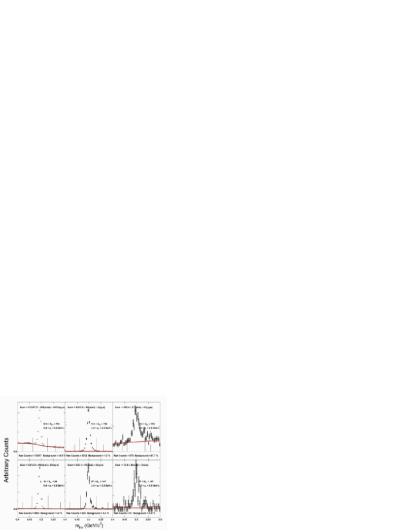
Figure 3: Invariant mass distributions for $\pi^{+}\pi^{-}$ from 0–5% central collisions (top) and 40–60% central collisions (bottom) in three $p_{T}$ intervals.

The observed masses, $496\pm 8$ MeV/$c^{2}$ for $\pi^{+}\pi^{-}$ and $1116\pm 4$ MeV/$c^{2}$ for $p\pi$, are roughly consistent with accepted values [GG00] and the widths are determined by the momentum resolution of the detector. For $p_{T}<1.5$ GeV/c, however, the $K_{S}^{0}$ peak is shifted to a lower mass. At $p_{T}=0.2$ GeV/c the peak is shifted by the greatest amount, 10 MeV/c. This shift is, for the most part, replicated by simulations and is attributed to energy loss suffered by the daughter particles in the detector material. Figure 3 shows invariant mass distributions for the $K_{S}^{0}$ $R_{CP}$ analysis. When the same selection criteria are used for all $p_{T}$ and centrality, the combinatorial background is larger for lower $p_{T}$ and for more central events. At higher $p_{T}$, where the size of our data sample is limited, we place less stringent requirements on the candidates. As a result, the combinatorial background is quite large in central events for $p_{T}>3.0$.

2 Detector, Tracking and Reconstruction Efficiency

Simulations are used to calculate the efficiency of the detector and the tracking software [Lon02]. The TPC response to Monte-Carlo generated $K_{S}^{0}$, $\Lambda$, or $\overline{\Lambda}$ decays is simulated. The simulated clusters (the pixel level TPC response) are then embedded into real events and these events are passed into the $K_{S}^{0}$, $\Lambda$, or $\overline{\Lambda}$ reconstruction chain. Reconstructed candidates are then associated with the embedded particles so that the efficiency of the detector and the reconstruction chain can be estimated.

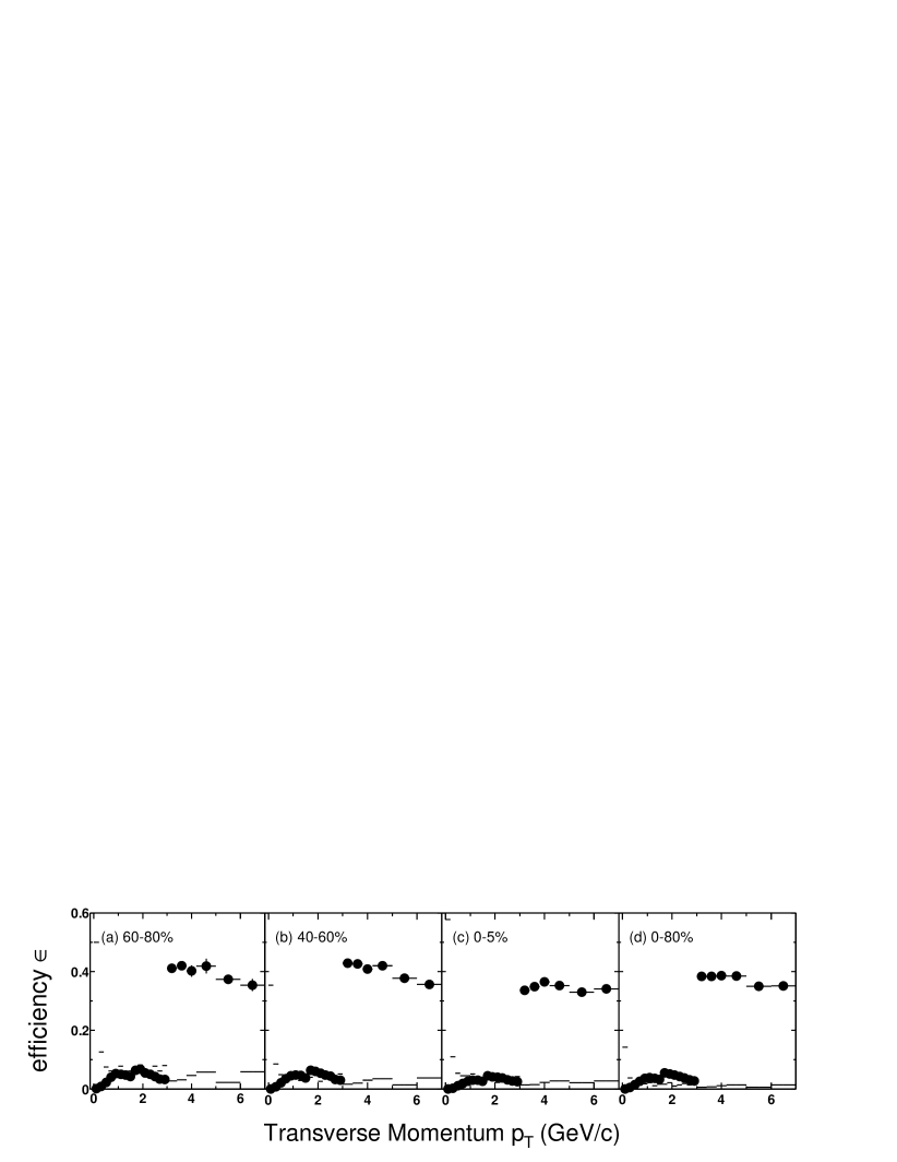
Figure 4: The $K_{S}^{0}$ efficiency for the selection criteria listed in Table 3. The discontinuities in the efficiency at $p_{T}=1.6$ and 3.0 GeV/c reflect changes in the selection criteria (see Table 3). The line histograms show the relative magnitude of the statistical error for the efficiency.

Figure 4 shows the efficiency correction factor for $K_{S}^{0}$ in the three centrality intervals used in the calculation of $R_{CP}$. The number of simulated $K_{S}^{0}$ particles we embed at a given $p_{T}$ is varied to approximate the true $p_{T}$ dependence of the yield. The slope of the $p_{T}$ spectrum is characterized by the inverse slope parameter T of an exponential fit. By matching the slopes in the simulations to the real slopes, the bin-sharing for the simulated particles replicates the bin-sharing for real particles. In this way, the efficiency correction also acts as a feed-down correction. With a slope on the embedded particle yield, it is necessary to embed within limited $p_{T}$ ranges to generate high statistics at large $p_{T}$. To match the feed-down in real data, simulated data cannot be used near the edge of the embedded $p_{T}$ range. Table 4 lists the slope parameters, the $p_{T}$ ranges, and the number of events used for the embedding.

Embedded $p_{T}$ range (GeV/c)	T (MeV/c2)	$p_{T}$ coverage (GeV/c)	Events
0.0–1.4	$300$	0.0–1.2	$39$ k
1.0–2.2	$315$	1.2–2.0	$45$ k
1.8–2.8	$330$	2.0–2.6	$49$ k
2.4–3.4	$330$	2.6–3.4	$36$ k
3.0–5.2	$450$	3.4–5.0	$15$ k
4.6–10.0	$500$	5.0–8.0	$19$ k

Table 4: Embedded data for $K_{S}^{0}$ analysis.

3 Systematic Uncertainties

Systematic errors for the spectra and $R_{CP}$ are introduced from uncertainties in the detection efficiency, the reconstruction efficiency, the background subtractions and from mis-measurements of the candidates $p_{T}$. The momentum resolution $\delta p_{T}/p_{T}$ is estimated from simulations. The other systematic uncertainties are studied by varying the $K_{S}^{0}$, $\Lambda$, and $\overline{\Lambda}$ selection criteria. Changing the selection criteria varies the number of background counts and tests how well the distributions in the simulated data match the real data. When all the relative distributions are accurately simulated, changing the cuts will not change the efficiency corrected particle yields.

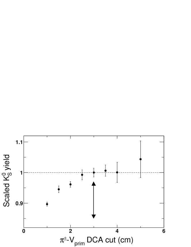
Figure 5: The $K_{S}^{0}$ yield for different $\pi^{\pm}-V_{prim}$ DCA selection criteria, relative to a 3.0 cm cut.

We found that the $K_{S}^{0}$ yield depends strongly on the $\pi^{\pm}-V_{prim}$ DCA cut. This variation is most likely caused by either space-charge or E$\times$B distortions which arise as ionization drifts toward the TPC pad planes. Figure 5 shows the measured $K_{S}^{0}$ yield for several $\pi^{\pm}-V_{prim}$ DCA values. The yields are scaled by the yield from the $\pi^{\pm}-V_{prim}$ DCA $>3.0$ cm analysis. No $p_{T}$ dependence is seen in the variation of the scaled yield, so the $p_{T}$ integrated yield is used in Figure 5. For 3.0 cm and above the yield is independent of the $\pi^{\pm}-V_{prim}$ DCA, so we used a 3 cm cut for our final analysis.

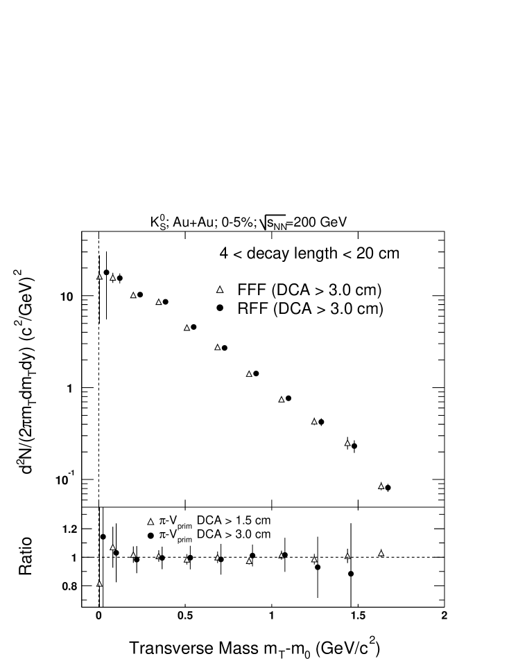
Figure 6: $K_{S}^{0}$ yield for forward and reversed field settings.

Figure 6 shows the $K_{S}^{0}$ spectra for forward and reversed field settings. Early in the analysis an approximately 8% systematic deviation was seen between the yields from events with the two field settings. By selecting only $K_{S}^{0}$ candidates with a decay length from 4–20 cm the deviation is removed. Final estimates for the systematic errors on $R_{CP}$ are dominated by variation in the yields with different selection criteria. Table 5 lists systematic uncertainties for $K_{S}^{0}$ and $\Lambda+\overline{\Lambda}$ $R_{CP}$.

	$K_{S}^{0}$						$\Lambda+\overline{\Lambda}$
$p_{T}$ (GeV/c)	1.	0	2.	5	4.	0	1.	0	2.	5	4.	0
$R_{CP}$ (bg)	$\pm 0$.	$04$	$\pm 0$.	$02$	$\pm 0$.	$08$	$\pm 0$.	$02$	$\pm 0$.	$04$	$\pm 0$.	$06$
$R_{CP}$ (eff)	$\pm 0$.	$10$	$\pm 0$.	$10$	$\pm 0$.	$10$	$\pm 0$.	$10$	$\pm 0$.	$10$	$\pm 0$.	$10$
$\delta p_{T}/p_{T}$	$\pm 0$.	$012$	$\pm 0$.	$027$	$\pm 0$.	$030$	$\pm 0$.	$016$	$\pm 0$.	$027$	$\pm 0$.	$037$

Table 5: The systematic errors from background (bg), and the efficiency calculation (eff) are listed for $R_{CP}$ (0–5%/40–60%) at three $p_{T}$ values along with the $p_{T}$ resolution ($\delta p_{T}/p_{T}$). The values listed are relative errors and do not include the overall normalization uncertainty in $R_{CP}$ from the calculation of $\mathrm{N_{bin}}$.

3 Reconstructing the Reaction Plane

The real reaction plane is not known, but the event plane, an experimental estimator of the true reaction plane, can be calculated from the azimuthal distribution of primary tracks [PV98]. The selection criteria for the primary tracks used to calculate the event plane are given in Table 2. We require the ratio of the number of space points to the expected maximum number of space points for each track to be greater than 0.52 to prevent split tracks from being counted twice. For the analysis using $\sqrt{s_{{}_{NN}}}=130$ GeV data the events are required to have a primary vertex within 75 cm longitudinally of the TPC center ($z$-vertex). During the Au+Au running with $\sqrt{s_{{}_{NN}}}=200$ GeV the $z$-vertex distribution was narrower so those events are required to have $|z$-vertex$|<25$ cm. These cuts do not bias our analysis.

For experiments at RHIC energies—unlike those at lower energies—the reaction plane is assumed to be transverse to the beam axis. As such, since it is not necessary to rotate the flow coordinate system in the polar direction, only the transverse direction is considered. The error introduced by this assumption will go as the square of the polar flow angle, $\theta_{Flow}\sim\langle p_{x}\rangle/p_{beam}\ll 1$, and is negligible.

With a perfect detector the azimuthal distribution of the event plane would be isotropic. In a realistic environment, however, limitations to a detectors acceptance lead to a bias in the estimation of the reaction plane. Acceptance corrections are introduced to account for both the limited coverage and the imperfect efficiency of a real detector. With the STAR detector, detector biases are removed from the event plane distribution by applying weights to the tracks used in its calculation. The $\mathbf{\phi}$-weights are generated by inverting the normalized $\phi$ distribution for tracks from many events. When other weights are included in the event plane calculation (e.g. $p_{T}$ weights) they are also applied to the $\phi$-weights. In this way, after the $\phi$-weights are applied the azimuthal distribution for tracks is—by construction—isotropic.

The acceptance of the STAR detector system depends on the kinematic variables of a particle ($\eta$, $\phi$ and $p_{T}$), the longitudinal position of the collision vertex in the TPC, the multiplicity of the event and the hour-by-hour state of the detector. During Run-2 electronics failures resulted in the temporary removal of read-out (RDO) boards from the data acquisition chain. The masking and unmasking of RDO boards changed the detectors acceptance with time. To ensure that all these variations are accounted for properly, the $\phi$-weights are calculated separately for positive or negative $\eta$, for positive or negative z-vertex position, for magnetic field polarity, for nine different centralities and for four different detector states.

Figure 7: An example of the weights used to correct the reaction plane calculation for acceptance is shown. These weights are for the centrality bin corresponding to 30–40% of the Au + Au collision cross-section and forward field polarity with the RDO board 3 in sector 9 and RDO board 4 in sector 21 where masked out.

Figure 7 shows examples of the $\phi$-weights. The 12-fold periodic structure is caused by the change in the detectors acceptance near the sector boundaries. The 24-fold periodic structure arises because a track that starts near the edge of a sector and curves toward the middle of the sector has a high probability of being reconstructed. As a consequence, the efficiency for detecting a positive particle is enhanced near the one side of a sector while the efficiency for detecting a negative particle is enhanced on the other side: two maxima are seen for each sector.

When the tracks in the event plane calculation are re-weighted properly the distribution of the azimuthal angle of the event plane is isotropic. Figure 8 (a) shows the event plane’s azimuthal distribution fit to a constant. When the event plane distribution is flat, the acceptance for the particles being compared to the event plane will not bias the measurement of $v_{2}$: as long as either the distribution of the event plane or the distribution of tracks is isotropic, acceptance effects introduce no bias. Poor acceptance will, however, negatively impact the reaction plane resolution. The decrease in the reaction plane resolution caused by the imperfect acceptance can be accounted for by applying a resolution correction factor to the measured $v_{2}$.

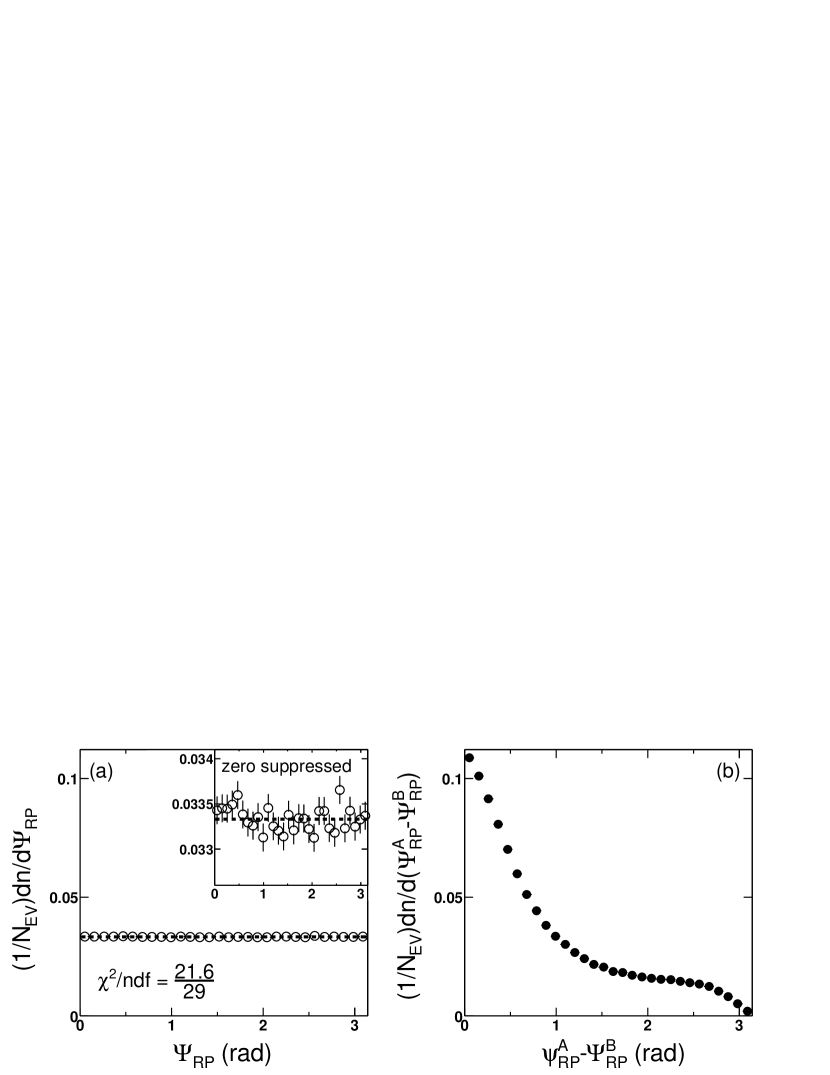
Figure 8: Left: Azimuthal distribution of the event plane fit to a constant. The event plane distribution should be ‘flat’ (azimuthally isotropic). Right: Distribution of the difference between the event-plane angles for sub-events of randomly assigned tracks.

A correction to the observed $v_{2}$ is introduced to account for the uncertainty in the determination of the reaction plane (i.e. the reaction plane resolution). The event plane (calculated from Equation 4) is used to estimate the reaction plane: the accuracy of the estimation depends on the number of tracks used and the magnitude of the true $v_{2}$ signal. With an infinite number of tracks, a finite $v_{2}$, and a perfect detector the event plane could be a perfectly accurate estimator of the true reaction plane. With a limited number of tracks detected in a real detector, however, we cannot assume that the true reaction plane has been accurately estimated. Poor resolution leads to a decrease in the calculated value of the flow parameters because, the correlation of the particles with the reaction plane is partially lost. The correction factor necessary to compensate for the resolution is found as follows:

$$v_{2}^{\Re}=\langle e^{2i(\phi-\Psi_{RP}^{\Re})}\rangle,v_{2}^{obs}=\langle e^{2i(\phi-\Psi_{EV})}\rangle$$ (1)

$$\frac{v_{2}^{\Re}}{v_{2}^{obs}}=\langle\exp^{2i(\Psi_{EP}-\Psi_{RP}^{\Re})}\rangle,$$ (2)

where $v_{2}^{\Re}$, $v_{2}^{obs}$, $\Psi_{RP}^{\Re}$, and $\Psi_{EP}$ are the real $v_{2}$, the observed $v_{2}$, the real reaction-plane angle, and the reconstructed event-plane angle. From Equation 2 the proper correction factor is found to be $\langle\cos 2(\Psi_{EP}-\Psi_{RP}^{\Re})\rangle$. This quantity can be calculated by reconstructing event planes from two random sub-sets of tracks within the same event (sub-events). The difference between the two sub-event-plane angles ($\Psi_{EP}^{A}-\Psi_{EP}^{B}$) is shown in Figure 8 (b). The resolution measured from two sub-events with equal numbers of tracks is given by Equation 3

$$\langle\cos\left[2\left(\Psi_{EP}^{A}-\Psi^{\Re}_{RP}\right)\right]\rangle=\sqrt{\langle\cos\left[2\left(\Psi_{EP}^{A}-\Psi_{EP}^{B}\right)\right]\rangle}.$$ (3)

The second harmonic sub-event-plane angles are calculated from Equation 4:

$$\tan\left(2\Psi_{EP}\right)=\frac{\sum_{i}w_{i}\sin\left(2\phi_{i}\right)}{\sum_{i}w_{i}\cos\left(2\phi_{i}\right)}.$$ (4)

The $w_{i}$’s in Equation 4 are weights used to maximize the resolution. In our case we use the particle’s transverse momentum and the $\phi$-weights as the weighting factor. An interpolation formula is then used with an iterative routine to calculate its roots and find the correction factor for the full event plane $\langle\cos 2(\Psi_{EP}-\Psi_{RP}^{\Re})\rangle$. We estimate the errors in the correction factor by varying the input by a small amount and calculating the change in the result.

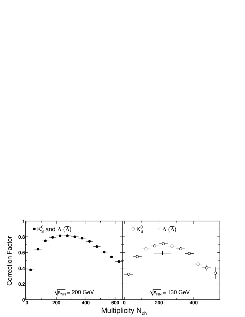
Figure 9: Left: Resolution correction factor for the $\sqrt{s_{{}_{NN}}}=200$ GeV analysis. Right: Resolution correction factor for the $\sqrt{s_{{}_{NN}}}=130$ GeV analysis. The increase in the resolution from Run-1 to Run-2 reflects the implementation of a new method (discussed in the text) for calculating the event plane. The resolution for the Run-1 $\Lambda$ analysis was lower than the $K^{0}_{S}$ analysis, only reaching a maximum of $0.58\pm 0.007$. With the new event plane calculation the resolution for $\Lambda$ and $K^{0}_{S}$ $v_{2}$ are the same and reach a maximum of $0.813\pm 0.003$.

The resolution correction factor is shown in Figure 9. The resolution depends on the number of tracks used and the magnitude of the event asymmetry. For the most peripheral events the small number of tracks available reduces the resolution while for the most central events the symmetry of the collision overlap region degrades it. As a result, the resolution is greatest at a centrality corresponding to roughly 20–30% of the collision cross-section.

Since $v_{2}$ is calculated from the distribution of ($\phi_{i}-\Psi_{RP}$), if particle $i$ is included in the evaluation of $\Psi_{RP}$, auto-correlations are introduced. For the measurement of $K_{S}^{0}$ $v_{2}$ in Run-1, these unwanted correlations are eliminated by calculating the event plane from charged particle tracks with a DCA to the primary vertex less than 1 cm while we use only tracks with a DCA greater than 1 cm to reconstruct the $K_{S}^{0}$. For $\Lambda$ we exclude from the event plane calculation all tracks identified as proton candidates by their energy loss in the TPC. This method has one important disadvantage: the reduction in the number of tracks used degrades the resolution of the reaction plane. This in turn leads to larger errors on the final $v_{2}$ measurement.

To maximize the number of tracks available for our event plane calculation, we implemented a new method to remove auto-correlations for neutral vertex particles. Rather than dividing tracks into two sets—one to be used for reconstructing neutral vertices and the other to be used for calculating the event plane—we calculate a separate event-plane angle for every $K^{0}_{S}$, $\Lambda$, or $\overline{\Lambda}$ candidate. Auto-correlations are removed by excluding only the two tracks associated with a specific $K_{S}^{0}$, $\Lambda$, or $\overline{\Lambda}$ from the event plane calculation. With a larger track sample the reaction plane resolution increases and the statistical and systematic uncertainty on $v_{2}$ decreases. Figure 9 shows the reaction plane resolution correction factor from the method used for the $\sqrt{s_{{}_{NN}}}=130$ GeV data and the method used for the $\sqrt{s_{{}_{NN}}}=200$ GeV data.

4 Calculating the $v_{2}$ of $K_{S}^{0}$ and $\Lambda+\overline{\Lambda}$

We use the measured yield within multiple intervals of $(\phi_{i}-\Psi_{RP}^{i})$ to calculate $v_{2}=\langle\cos\left[2(\phi_{i}-\Psi_{RP}^{i})\right]\rangle$, where $\phi_{i}$ is the azimuth angle of the momentum vector of particle $i$ and $\Psi_{RP}^{i}$ is the reaction-plane angle for the event that particle $i$ was observed in. To remove autocorrelations, the contributions from the decay daughter tracks associated with particle $i$ are subtracted from the right hand side of Equation 4. The candidates are categorized by invariant mass, $p_{T}$ and $(\phi_{i}-\Psi_{RP}^{i})$. For each $p_{T}$ interval, twenty $(\phi-\Psi^{RP})$ intervals from 0 to 2$\pi$ are created (all events are combined). The yield in interval $j$ ($dn_{j}$) is calculated by fitting a smooth function to the mass region outside the candidate mass window and integrating the number of counts above this background. To minimize the systematic errors associated with fitting the background, the same background shape is used for every $j$ $(\phi-\Psi^{RP})$ interval: only the relative amplitude of the background is allowed to change. Once the yields are known, we calculate $v_{2}(p_{T})$ using

$$v_{2}(p_{T})=\frac{\sum_{j}dn_{j}\cos 2\left[\left(\phi-\Psi^{RP}\right)_{j}\right]}{\sum_{j}dn_{j}}.$$ (5)

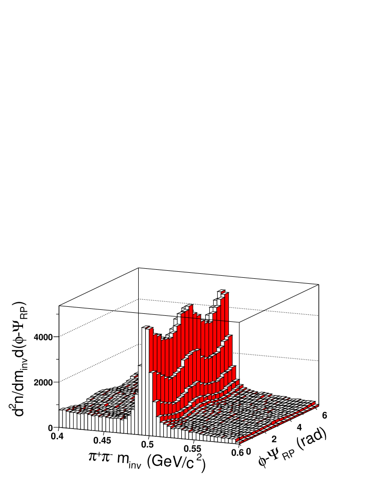
Figure 10: Distribution of $K_{S}^{0}$ candidates in the invariant mass versus ($\phi-\Psi^{RP}$) plane.

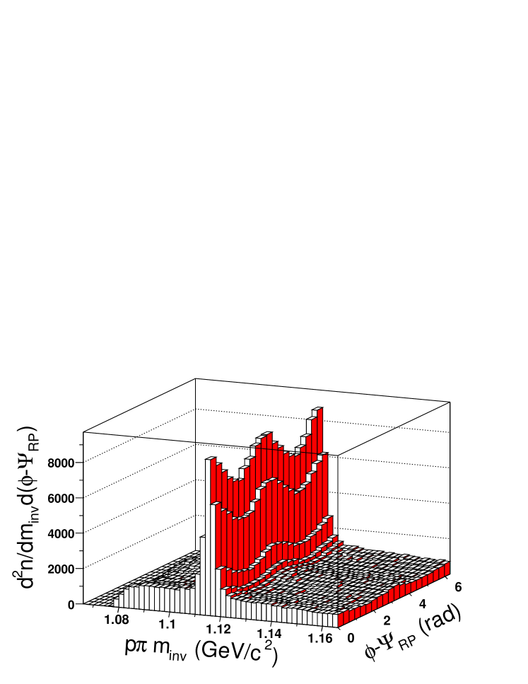
Figure 11: Distribution of $\Lambda$ and $\overline{\Lambda}$ candidates in the invariant mass versus ($\phi-\Psi^{RP}$) plane.

Figure 10 shows the $p_{T}$ inclusive distribution of the $K_{S}^{0}$ candidates in the invariant mass versus $(\phi-\Psi_{RP})$ plane. The $v_{2}$ signal—an enhancement near zero, $\pi$ and $2\pi$ radians—is clearly visible. We find our method of calculating $v_{2}$ is insensitive to the background contamination, so, to maximize our statistical sample, we use relatively loose selection criteria for the identification of $K_{S}^{0}$, $\Lambda$, and $\overline{\Lambda}$ candidates. Table 6 lists the criteria used for the final analysis. Figure 11 shows the same distribution for $\Lambda$ and $\overline{\Lambda}$ candidates.

	$K_{S}^{0}$			$(\Lambda)$
$p_{T}$ (GeV/c)	$<0.6$	$0.6-2.0$	$>2.0$	$<2.0$	$>2.0$
$\pi^{+}(p)$–$\pi^{-}$ DCA	$<0.70$	$<0.70$	$<0.80$	$<0.70$	$<0.70$
$\pi^{+}(p)$–$V_{prim}$ DCA	$>1.50$	$>1.50$	$>0.35$	$>0.50$	$>0.25$
$\pi^{-}$–$V_{prim}$ DCA	$>1.50$	$>1.50$	$>0.35$	$>1.00$	$>1.00$
Decay Length	$>3.50$	$>5.50$	$>7.00$	$>4.50$	$>4.50$
$V^{0}-V_{prim}$ DCA	$<0.70$	$<0.70$	$<0.80$	$<0.70$	$<0.70$

Table 6: The vertex and daughter track selection criteria for $K_{S}^{0}$, and $\Lambda$. For $\overline{\Lambda}$ criteria are the same as $\Lambda$ with the $p(\pi^{-})$ exchanged with $\overline{p}(\pi^{+})$. All units are centimeters unless indicated otherwise.

1 Systematic Uncertainties and Correlations Unrelated to the Reaction Plane

	$K_{S}^{0}$						$\Lambda+\overline{\Lambda}$
$p_{T}$ (GeV/c)	1.	0	2.	5	4.	0	1.	0	2.	5	4.	0
$v_{2}$ (bg)	$+0$.	$000$	$+0$.	$001$	$+0$.	$003$	$+0$.	$001$	$+0$.	$005$	$+0$.	$005$
	$+0$.	$001$	$-0$.	$007$	$-0$.	$018$	$-0$.	$007$	$-0$.	$001$	$-0$.	$001$
$v_{2}$ (n-f)	$+0$.	$00$	$+0$.	$00$	$+0$.	$00$	$+0$.	$00$	$+0$.	$00$	$+0$.	$00$
	$-0$.	$01$	$-0$.	$04$	$-0$.	$03$	$-0$.	$01$	$-0$.	$04$	$-0$.	$04$
$\delta p_{T}/p_{T}$	$\pm 0$.	$012$	$\pm 0$.	$027$	$\pm 0$.	$030$	$\pm 0$.	$016$	$\pm 0$.	$027$	$\pm 0$.	$037$

Table 7: The systematic errors from background (bg) and non-flow effects (n-f) are listed for $v_{2}$ (0–80%) at three $p_{T}$ values along with the $p_{T}$ resolution ($\delta p_{T}/p_{T}$). The values listed are absolute errors.

Sources of systematic error in the calculation of $v_{2}$ are correlations unrelated to the reaction plane (non-flow effects), estimation of the yield from the invariant mass distributions, the $p_{T}$ resolution ($\delta p_{T}/p_{T}$), and biases introduced by the cuts used in the analysis. Table 7 lists the dominant systematic errors for $K_{S}^{0}$ and $\Lambda+\overline{\Lambda}$ $v_{2}$. The systematic error in $v_{2}$ associated with the yield extraction is found to be small and the non-flow systematic error is dominant.

The magnitude of charged particle $v_{2}$ absent of non-flow effects has been estimated using a four-particle cumulant analysis [Adl02c]: a method thought to be less sensitive to non-flow correlations. Figure 12 (a) shows the ratio of $v_{2}$ from a four particle cumulant analysis and a two particle cumulant analysis. The two particle cumulant $v_{2}$ result has been shown to be similar to—but slightly larger than—the $v_{2}$ from a reaction plane analysis [Adl02c]. Figure 12 suggests that for minimum-bias collisions, non-flow correlations may account for 10–20% of the charged particle $v_{2}$.

The four-particle cumulant method can be adapted to study $v_{2}$ for $\Lambda+\overline{\Lambda}$ and $K_{S}^{0}$ absent of non-flow contributions but, to be decisive, will require a large data sample. Nuclear modification of jet production and fragmentation could lead to a particle-type dependence in the relative fraction of the non-flow contribution to $v_{2}$. At $p_{T}>3$ GeV, jet production is thought to be a likely source of non-flow correlations. The effect of standard jet fragmentation on $v_{2}$ was examined using superimposed p+p collisions generated with PYTHIA [Sjo01]. Within the measured $p_{T}$ region, no significant difference is seen between $\Lambda+\overline{\Lambda}$ and $K_{S}^{0}$ non-flow from this source. As such, in this analysis, we assume a similar magnitude for the non-flow contribution to the $v_{2}$ of $\Lambda+\overline{\Lambda}$ and $K_{S}^{0}$.

Figure 12: Left: Ratio of $v_{2}$ calculated by the fourth-order cumulant method and the reaction plane method [Adl02c]. Right: Integrated $v_{2}$ as a function of centrality for each method [Adl02c].

Figure 12 (b) shows the integrated $v_{2}$ versus centrality ($\mathrm{N_{ch}/N_{max}}$) from Reference [Adl02c], where $v_{2}$ calculated using a four particle cumulant analysis is compared to $v_{2}$ from a reaction plane analysis. Table 8 lists the values of $\mathrm{N_{ch}}$ and the collision cross-sections corresponding to the $x$-axis in Figure 12 (b) [Adl02c]. The difference between the $v_{2}$ calculated from these methods is used to estimate the centrality dependence of non-flow effects. The cumulant analysis indicates that non-flow effects are largest in the most central and most peripheral events. Some or all of the difference between these methods could, however, arise from event-by-event fluctuations in the initial source shape: these fluctuations would reduce the value of $v_{2}$ calculated from the cumulant analysis. As such, the cumulant analysis and the reaction plane analysis are often taken as estimates of the upper and lower limits on the true $v_{2}$.

$\mathrm{N_{ch}/N_{max}}$	0.849	0.708	0.590	0.472	0.363	0.258	0.160	0.060
X-section (%)	0–5	5–10	10–16	16–24	24–31	31–41	41–53	53–77

Table 8: Percent of the collision cross-section corresponding to $\mathrm{N_{ch}/N_{max}}$. The value of $\mathrm{N_{max}}$ is approximately 878.

Chapter 3 Results

As shown in Figure 4, $K_{S}^{0}$, $\Lambda$ and $\overline{\Lambda}$ particles were identified during Run-2 across a broader $p_{T}$ range than any other particle. In this chapter we present the measurement of $v_{2}$ for $K_{S}^{0}$ and $\Lambda+\overline{\Lambda}$ at mid-rapidity from Au+Au collisions at $\sqrt{s_{{}_{NN}}}=130$ and 200 GeV. The $p_{T}$ spectra are shown for 0–5%, 40–60%, and 60–80% centrality intervals. The centrality dependence is studied via the nuclear modification factor $R_{CP}$ which is derived from the spectra.

1 Elliptic Flow

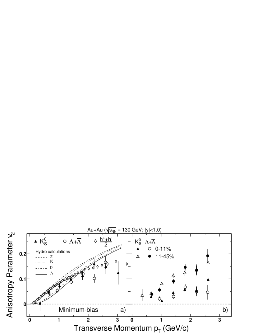
Figure 1: Elliptic flow for $K_{S}^{0}$ and $\Lambda+\overline{\Lambda}$ particles at mid-rapidity in Au+Au collisions at $\sqrt{s_{{}_{NN}}}=130$ GeV.

Elliptic flow at mid-rapidity as a function of transverse momentum for minimum-bias (a), 0–11% central and 11–45% central (b) Au+Au collisions at $\sqrt{s_{{}_{NN}}}=130$ GeV is shown in Figure 1. The $v_{2}$ of $K_{S}^{0}$ and the $v_{2}$ of $\Lambda+\overline{\Lambda}$ both increase monotonically with $p_{T}$ in the 11–45% centrality interval. Throughout the measured $p_{T}$ range, the $v_{2}$ for both particles is larger in more peripheral collisions than in the central collisions. A similar dependence was observed for charged particles in Au + Au collisions at the same RHIC energy [Ack01]. Also shown in the figure is $v_{2}(p_{T})$ for charged hadrons [Adl03a] and hydrodynamic model calculations. Within statistical uncertainty, the minimum-bias $K_{S}^{0}$ results are in agreement with the $v_{2}$ of charged kaons (not shown) [Adl01]. We observe that $v_{2}$ for both strange particles increases as a function of $p_{T}$ up to about 1.5 GeV/c, similar to the hydrodynamic model prediction. For $p_{T}~{}\geq~{}2$ GeV/c however, the values of $v_{2}$ seem to be saturated. It has been suggested that the shape and height of $v_{2}$ above 2–3 GeV/c in a pQCD model is related to energy loss in an early, high-parton-density, stage of the evolution [GVW01].

These are the first measurements of $v_{2}$ for $K_{S}^{0}$ and $\Lambda+\overline{\Lambda}$ at RHIC energy and the first measurement of $v_{2}$ for any identified particle above $p_{T}\sim 1.0$ GeV/c. The statistical sample for Run-1, however, is limited and several important details remain to be studied—how well do the hydrodynamic models reproduce the mass dependence for $K_{S}^{0}$ and $\Lambda+\overline{\Lambda}$, does $v_{2}$ for all particles saturate with the same magnitude at the same $p_{T}$, and does the relative strangeness content of the particle affect its elliptic flow? For Run-2, improvements were made to the analysis technique and a larger data set became available.

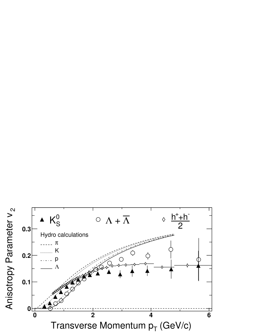
Figure 2: The minimum-bias (0–80% of the collision cross-section) $v_{2}(p_{T})$ for $K_{S}^{0}$, $\Lambda+\overline{\Lambda}$ and $h^{\pm}$ at mid-rapidity in Au+Au collisions at $\sqrt{s_{{}_{NN}}}=200$ GeV. The error bars shown are statistical only. Hydrodynamical calculations of $v_{2}$ for pions, kaons, protons and lambdas are also plotted [HKH01].

Figure 2 shows minimum-bias $v_{2}$ at $\sqrt{s_{{}_{NN}}}=200$ GeV for $K_{S}^{0}$, $\Lambda+\overline{\Lambda}$ and charged hadrons $h^{+}+h^{-}$. The analysis of the charged hadron $v_{2}$ is described in Reference [Adl03a]. The curves in the figure represent hydrodynamic model calculations of $v_{2}$ for pions, kaons, protons, and lambdas [HKH01]. At low $p_{T}$, the model calculations are in good agreement with the mass and $p_{T}$ dependence of $v_{2}$. At intermediate $p_{T}$ however, we find $v_{2,\Lambda+\overline{\Lambda}}>v_{2,K}$ in contradiction to hydrodynamical calculations: where at a given $p_{T}$, heavier particles have smaller $v_{2}$ values. The $p_{T}$-scale where $v_{2}$ deviates from the hydrodynamical prediction is $\sim 2.5$ GeV/c for $\Lambda+\overline{\Lambda}$ and $\sim 1$ GeV/c for $K_{S}^{0}$. Our measurement at $\sqrt{s_{{}_{NN}}}=200$ GeV establishes the particle-type dependence of the $v_{2}$ saturation at intermediate $p_{T}$ ($1.5<p_{T}<4.0$ GeV/c).

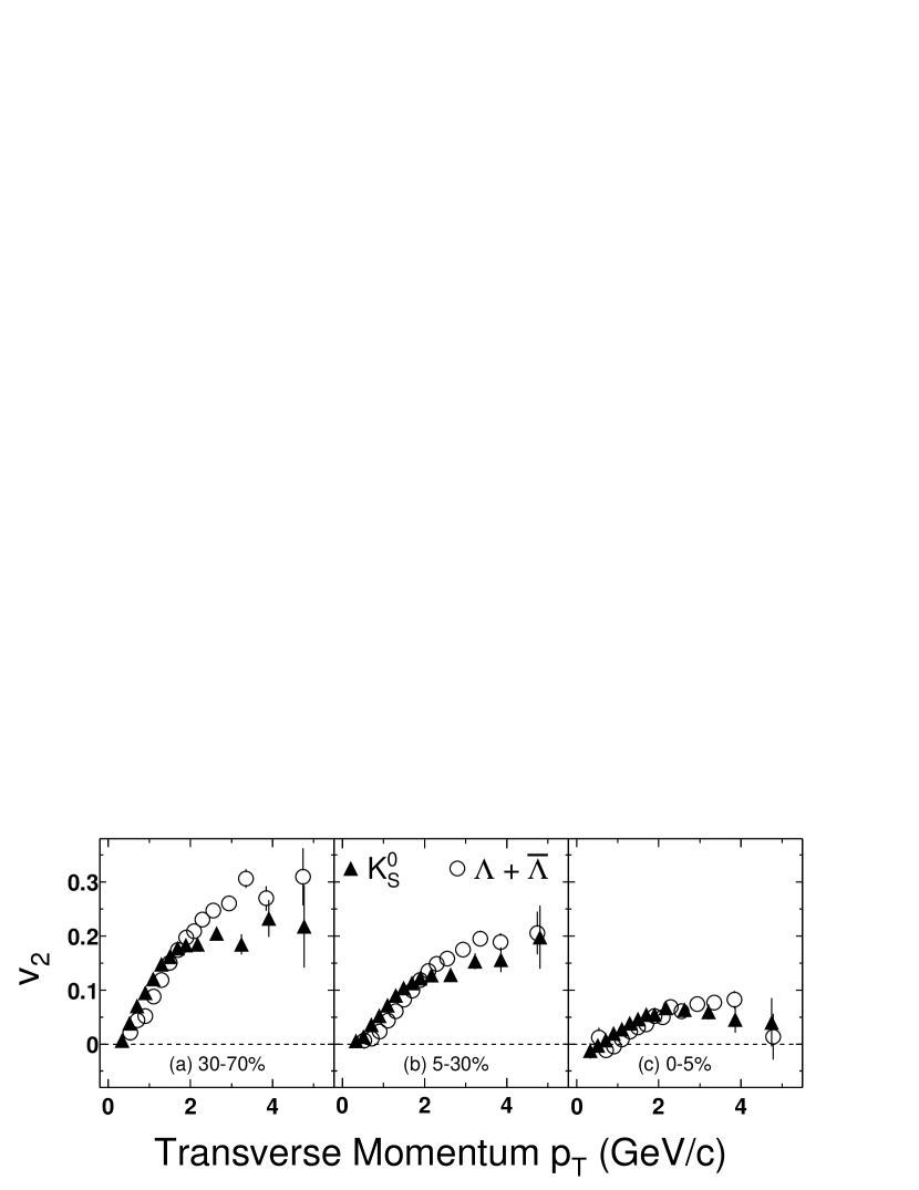
Figure 3: The $v_{2}$ of $K_{S}^{0}$ and $\Lambda+\overline{\Lambda}$ at $\sqrt{s_{{}_{NN}}}=200$ GeV as a function of $p_{T}$ for 30–70%, 5–30% and 0–5% of the collision cross-section. The error bars represent statistical errors only. The non-flow systematic errors for the 30–70%, 5–30% and 0–5% centralities are -25%, -20% and -80% respectively.

Figure 3 shows $v_{2}$ of $K_{S}^{0}$ and $\Lambda+\overline{\Lambda}$ at mid-rapidity for Au+Au collisions at $\sqrt{s_{{}_{NN}}}=200$ GeV as a function of $p_{T}$ for three centrality intervals: 30–70%, 5–30%, and 0–5% of the geometrical cross-section. The $p_{T}$ dependence of $v_{2}$ from all three centrality bins has a similar trend: a monotonic rise with $p_{T}$ at low $p_{T}$ and a saturation at intermediate $p_{T}$. The saturation of $v_{2}$ in the intermediate $p_{T}$ region from minimum-bias trigger data in Figure 2 is not due to the superposition of drastically different $p_{T}$ dependencies for various centrality bins. The values of $v_{2}$ at saturation show a particle-type and centrality dependence.

2 Spectra

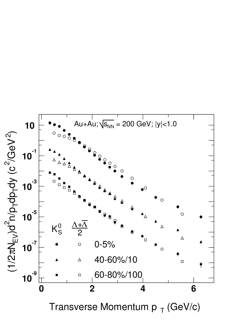
Figure 4: Spectra for $K_{S}^{0}$ and $\Lambda+\overline{\Lambda}$ [Lon03] at mid-rapidity from central and peripheral Au+Au collisions at $\sqrt{s_{{}_{NN}}}=200$ GeV.

In Figure 4 we show the spectra for $K_{S}^{0}$ and $\Lambda+\overline{\Lambda}$ [Lon03] at mid-rapidity in Au+Au collisions at $\sqrt{s_{{}_{NN}}}=200$ GeV. At $p_{T}\sim 1.5$ and 4.5 GeV/c, the $K_{S}^{0}$ and $\Lambda+\overline{\Lambda}$ yields coincide. In the intermediate $p_{T}$ region, a greater number of $\Lambda+\overline{\Lambda}$ particles are produced than $K_{S}^{0}$ particles. The $K_{S}^{0}$ spectra show a clear hardening at higher $p_{T}$ while the $\Lambda+\overline{\Lambda}$ spectra appears to remain soft within most of the measured $p_{T}$ range. As a result, the number of $K_{S}^{0}$ particles produced becomes larger than the number of $\Lambda+\overline{\Lambda}$ particles again for $p_{T}>4.5$ GeV/c. For peripheral collisions the separation at intermediate $p_{T}$ between the $K_{S}^{0}$ and $\Lambda+\overline{\Lambda}$ yields appears much smaller than in central collisions. The nuclear modification factor $R_{CP}$ is a useful measure for studying the relative centrality dependencies.

3 Nuclear Modification $R_{CP}$

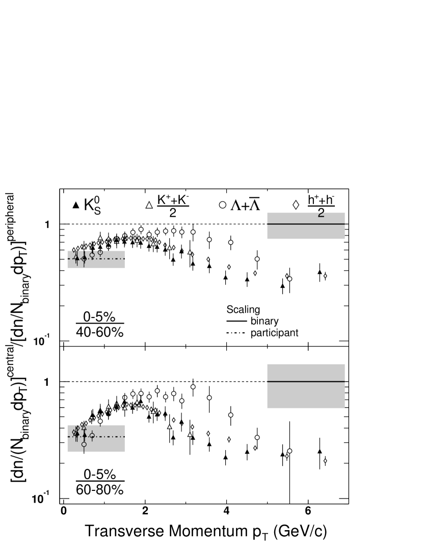
Figure 5: Nuclear modification of $K_{S}^{0}$ and $\Lambda+\overline{\Lambda}$ production at mid-rapidity for Au+Au collisions at $\sqrt{s_{{}_{NN}}}=200$ GeV. For comparison, the $R_{CP}$ for charged kaons is also shown where the kaons have been identified from single-prong decays (kinks) as discussed in Reference [Adl02d].

Figure 5 shows $R_{CP}$ for $K_{S}^{0}$, and $\Lambda+\overline{\Lambda}$ using the 5% most central collisions, normalized by peripheral collisions (40–60% and 60–80%). For reference, the charged kaon and charged hadron $R_{CP}$ are also shown. For charged hadrons, these $40$-$60\%$ and $60$-$80\%$ bins have been shown to approximately follow binary collision scaling (relative to p+p collisions) without medium modification [Ada03b]. The bands in Figure 5 represent the expected values of $R_{CP}$ for binary and participant ($\mathrm{N_{part}}$) scaling including systematic variations from the calculation [Ada03b]. Table 1 gives the values for $\mathrm{N_{bin}}$ and $\mathrm{N_{part}}$

Cross-section (%)	0–5	40–60	60–80
$\langle\mathrm{N_{bin}}\rangle$	$990^{+67}_{-67}$	$91.8^{+22}_{-23}$	$20.0^{+7}_{-9}$
$\langle\mathrm{N_{part}}\rangle$	$352^{+6}_{-7}$	$61.0^{+10}_{-10}$	$19.8^{+5}_{-6}$

Table 1: Monte-Carlo Glauber model calculations of the number of participating nucleons $\mathrm{N_{part}}$ and the number of binary nucleon-nucleon collisions $\mathrm{N_{bin}}$ for three centrality intervals [Ada03b].

The kaon and (anti-)lambda yields are suppressed by different magnitudes and the $p_{T}$-scales associated with the onset of the high $p_{T}$ suppression are different. $R_{CP}$ for kaons increases with $p_{T}$ from the participant scaling limit, reaches a maximum of approximately 0.6 at $p_{T}\sim 1.6$ GeV/c and then decreases with $p_{T}$. The $R_{CP}$ for $\Lambda+\overline{\Lambda}$, however, rises to a maximum of approximately 0.9 at $p_{T}\sim 2.0$ GeV/c, remains near that value up to $p_{T}\sim 3.5$ GeV/c and then decreases with $p_{T}$. For most of the intermediate $p_{T}$ region, $\Lambda+\overline{\Lambda}$ $R_{CP}$ within errors coincides with binary collision scaling, while the kaon $R_{CP}$ is significantly below unity. For both species, the $p_{T}$ where $R_{CP}$ begins to decrease approximately coincides with the $p_{T}$ where $v_{2}$ in Figure 2 saturates. At high $p_{T}$ ($p_{T}>5.0$ GeV/c), $R_{CP}$ values for $K_{S}^{0}$ and $\Lambda+\overline{\Lambda}$ are approaching the value of the charged hadron $R_{CP}$. The apparent disappearance of the particle-type dependence of $R_{CP}$ may signify that single parton fragmentation dominates the features of $R_{CP}$ above $p_{T}\sim 5$ GeV/c.

Chapter 4 Discussion

Event-by-event azimuthal anisotropy in particle production is thought to probe the early stages of relativistic heavy-ion collisions [Oll92]. For $p_{T}<1.0$ GeV/c, hydrodynamic models [HKH01] describe $v_{2}$ [Ack01, Adl01], and the particle spectra [KH03] well. These models predict that $v_{2}$ will rise monotonically with $p_{T}$. It is expected however, that for particles with large $p_{T}$ the model assumptions will break down. Measurements using charged particles and our measurements using $K_{S}^{0}$ and $\Lambda+\overline{\Lambda}$ do indeed indicate a saturation of $v_{2}$—well below the hydrodynamic calculations—at intermediate $p_{T}$. The nuclear modification factor $R_{CP}$ for charged particles also shows a large $p_{T}$-independent suppression of particle production at $p_{T}>4.5$ GeV/c. Models based on parton energy loss [GVW01, Shu02] and transport opacity [MG02] have been discussed in relation to the saturation and centrality dependence of $v_{2}$ at intermediate and high $p_{T}$. The authors of Reference [GVW02] propose that the saturation of charged particle $v_{2}$ could be a consequence of the transition from soft to hard production processes occurring at different $p_{T}$-scales for pions and protons.

We show here that the extent of the $p_{T}$ region where hydrodynamic like processes (or other soft processes) dominate the spectrum is particle species dependent. In Chapter 3, we reported the measurement of $v_{2}$ and $R_{CP}$ for $K_{S}^{0}$ and $\Lambda+\overline{\Lambda}$. These measurements show that for $p_{T}$ up to 3 GeV/c $\Lambda+\overline{\Lambda}$ $v_{2}$ continues to rise—similar to hydrodynamic model calculations—while the $K_{S}^{0}$ $v_{2}$ saturates at $p_{T}\sim 1.5$ GeV/c. We also find that there is a particle-type dependence to the onset of the suppression—as measured by $R_{CP}$—of $K_{S}^{0}$ and $\Lambda+\overline{\Lambda}$ production. In addition, for each particle the lower $p_{T}$ bound of the suppressed region of $R_{CP}$ coincides with the lower bound of the saturated region of $v_{2}$.

It has been suggested that if a partonic state exists prior to hadronization, the process of particle formation at intermediate $p_{T}$, by string fragmentation, parton fragmentation [LK02b] or quark coalescence [LK02a, LM03, HY03, GKL03a, FMN03b, FMN03a], may lead to a dependence of $v_{2}$ and $R_{AA}$ on particle type. In this case, it is possible that these measurements will provide information on the existence and nature of an early partonic state. In this chapter we investigate the interplay between the apparently soft and hard components of the $K_{S}^{0}$ and $\Lambda+\overline{\Lambda}$ spectrum and explore possible sources for the particle-type dependence of our measurements. We begin with a brief description of hydrodynamic and energy loss models and we compare their predictions to our data. In Section 3 we use hydrodynamical inspired and pQCD inspired fits to estimate the $p_{T}$ where soft, hydrodynamical-type processes are no longer appreciable.

1 Describing Heavy-Ion Collisions with Hydrodynamics

A system can be described within a hydrodynamical formalism when the time scales of its microscopic processes are sufficiently smaller than the time scale for its macroscopic evolution. For heavy-ion collisions this means the time between interactions amongst the constituents—partonic and/or hadronic—must be much smaller than the lifetime of the system. When this condition is met, the constituents can interact enough times to equilibrate. The space-time evolution of the system can then be described in the framework of relativistic fluid dynamics. The equations of motion are derived from the conservation of energy and momentum $\partial_{\mu}T^{\mu\nu}=0$. The energy-momentum tensor $T^{\mu\nu}$ in the ideal fluid approximation is given by:

$$T^{\mu\nu}=(\epsilon+p)u^{\mu}u^{\nu}-pg^{\mu\nu},$$ (1)

where $\epsilon$, $p$, and $u^{\mu}$ are respectively the energy density, pressure, and four velocity.

Prior to the onset of local equilibrium, the hydrodynamical equations are invalid. As such, they can only describe heavy-ion collisions from an initial time $\tau_{0}$ until the time when interaction rates in the system become too small and local thermal equilibrium can no longer be maintained (i.e the freeze-out time). The initialization of the hydrodynamic evolution requires that the pre-thermalization stage be modelled so that the initial conditions can be estimated. Given a set of initial conditions and the hydrodynamic equations, all that remains to be specified is the nuclear equation-of-state EOS which relates the thermodynamic quantities of the system. The EOS can be modelled or calculated using lattice QCD. Finding the EOS that governs nuclear matter at high temperature and density is the primary objective of heavy-ion physics and hydrodynamical model calculations may provide insight into its form.

The hydrodynamic equations for an ideal fluid describe the velocity and pressure fields for thermalized fluid elements. The Cooper-Frye formula [CF74] is used to calculate the momentum distribution for the hadrons created from the fluid elements on the freeze-out hyper-surface $\Sigma$:

$$E\frac{dn_{i}}{d^{3}p}=\frac{d_{i}}{(2\pi)^{3}}\int_{\Sigma}\frac{p^{\mu}d\sigma_{\mu}}{\exp[(p^{\mu}u_{\mu}-\mu_{i})/T^{th}]\mp 1},$$ (2)

where $d_{i}$ is a degeneracy factor, $\mu_{i}$ are the chemical potentials for the hadrons, $p^{\mu}$ are their four momentum, and $d\sigma_{\mu}$ is the outward normal vector on $\Sigma$. Hydrodynamic models have been particularly successful in reproducing the mass dependence of $v_{2}$ at low $p_{T}$. Figure 1 shows $v_{2}$ versus $p_{T}$ (left) and the integrated $v_{2}$ versus particle mass for identified particles (right) compared to hydrodynamical model calculations. In these models the increase in the integrated $v_{2}$ with mass is a consequence of the collective motion of the fluid elements built up as the system interacts and expands. When particles with more mass freeze-out from fluid elements flowing with a given velocity, they will carry greater momenta. In this way, an anisotropic collective flow velocity at freeze-out leads to an increase of the integrated $v_{2}$ with particle mass. This increase and the mass dependence of the differential $v_{2}$ both indicate that a significant collective motion is established—perhaps early in the collision—and that the source eccentricity is efficiently transferred to momentum-space anisotropy.

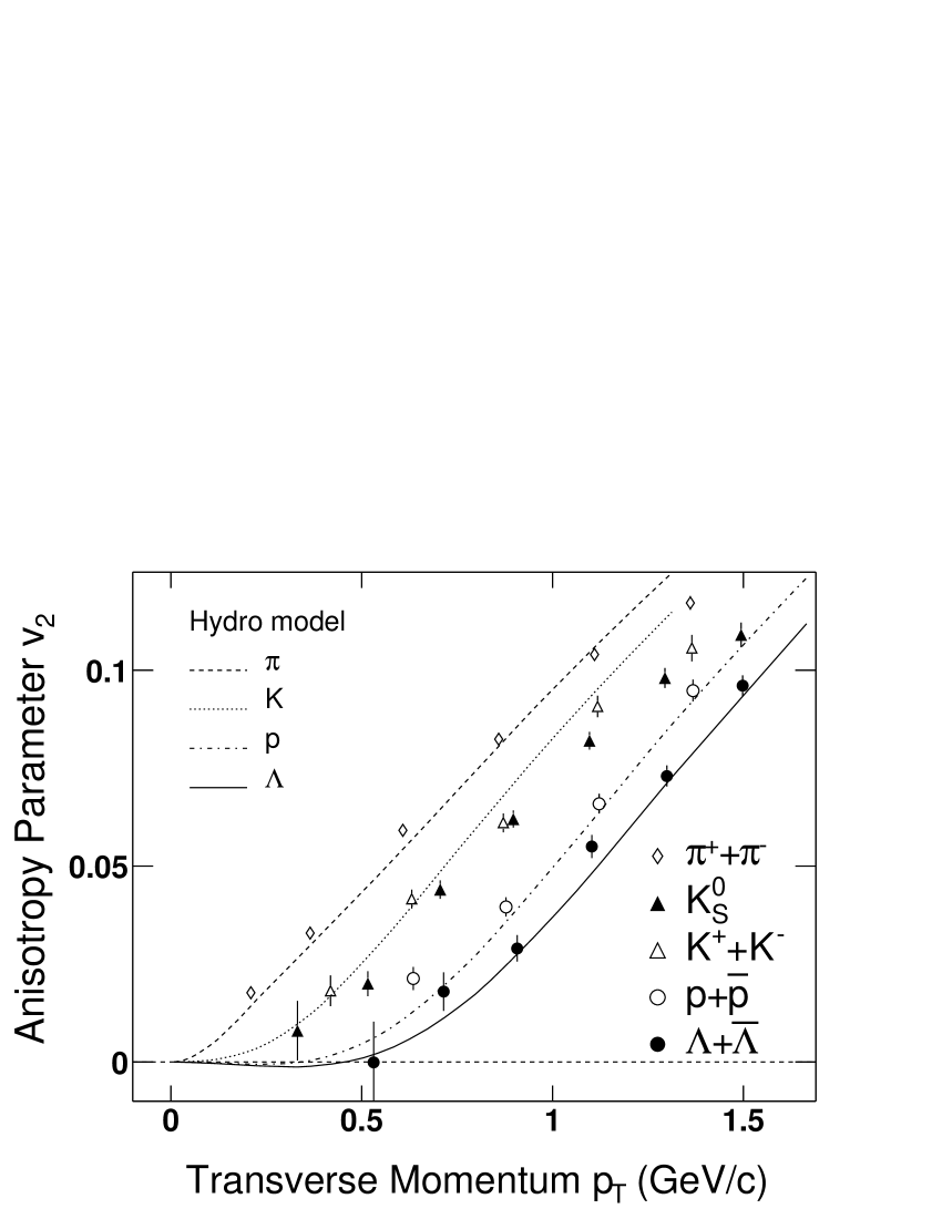
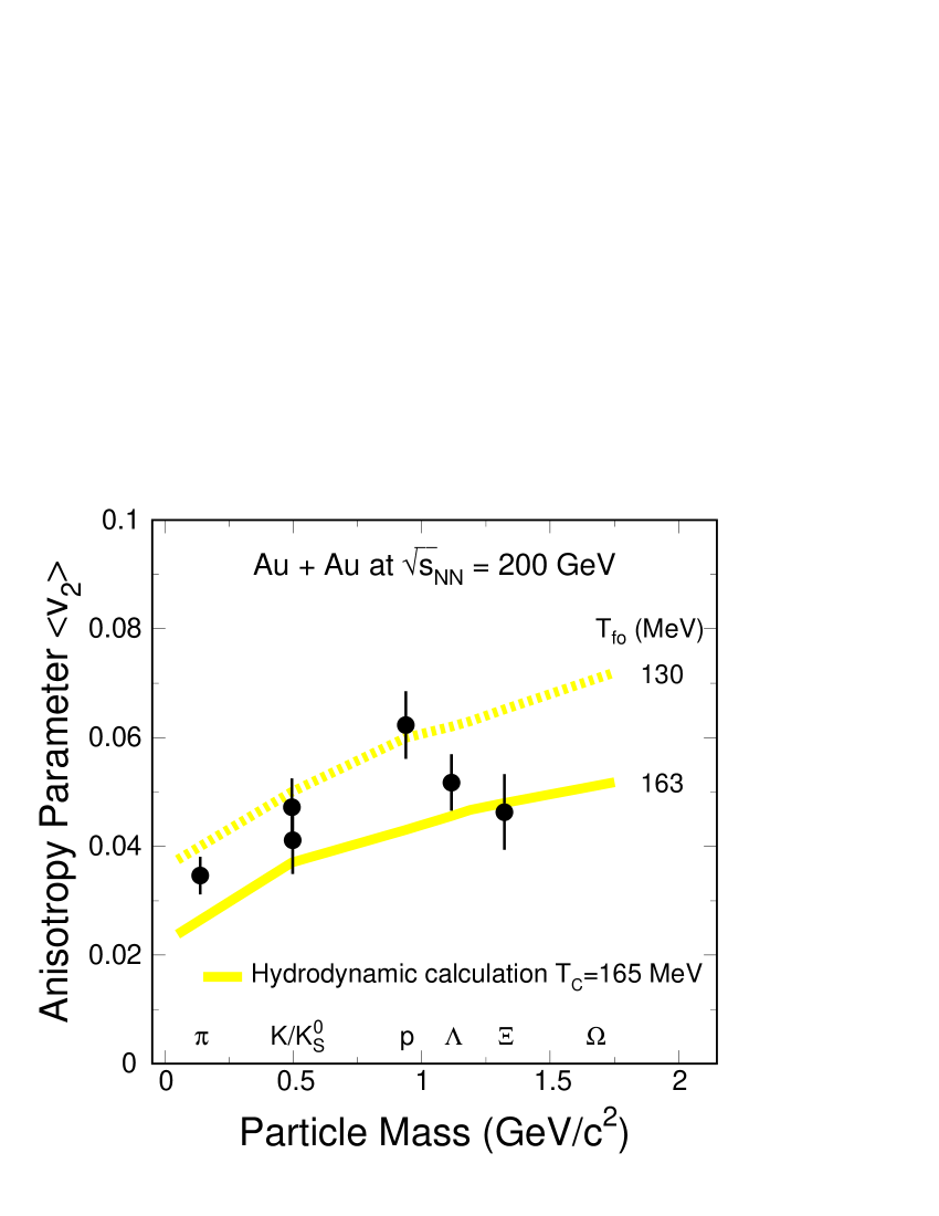
Figure 1: Left: Differential $v_{2}$ at low $p_{T}$ for pions, kaons, protons, and lambdas at mid-rapidity from Au+Au collisions at $\sqrt{s_{{}_{NN}}}=200$ GeV. The charged pion, charged kaon, and the proton $v_{2}$ were measured by the PHENIX collaboration [Esu03]. Right: Integrated $v_{2}$ versus mass compared to hydrodynamic calculations with different freeze-out temperatures. The integrated $v_{2}$ is calculated by weighting the measured $v_{2}$ with the particle yield extracted from fits to the spectra.

The results of a full hydrodynamical model calculation can be approximated with a simple analytical model: the blast wave model [HKH01]. The equations of the blast wave model describe particle emission from a thin cylindrical shell of thermalized matter with temperature $T$. The particle production is approximated by a boosted Boltzmann distribution so that the particle spectra can be calculated from the equations:

$$\frac{d^{3}n}{dp^{3}}\sim\int_{0}^{2\pi}d\phi_{s}K_{1}(\beta(\phi_{s}))e^{\alpha(\phi_{s})\cos(\phi_{s}-\phi_{p})},$$ (3)

$$\alpha(x,p)=\frac{p_{T}}{T\sinh(\rho(x))},$$

$$\beta(x,p)=\frac{m_{T}}{T\cosh(\rho(x))},$$

where $\phi_{p}=\tan^{-1}(p_{y}/p_{x})$, and $\phi_{s}=\tan^{-1}(y/x)$ are respectively the momentum and coordinate space azimuthal freeze-out angles, $K_{1}$ is the modified Bessel’s function and $\rho(x)$ is the transverse flow rapidity. In Section 3 we’ll use the blast wave equations to parameterize the soft part of the $K_{S}^{0}$ and $\Lambda+\overline{\Lambda}$ spectrum.

2 Energy Loss

For p+p collisions, when scatterings involve sufficiently large momentum transfer, pQCD calculations describe hadron production well (see Figure 1). To relate the partonic and hadronic invariant cross-sections ($E_{a}\frac{d^{3}n_{a}}{dp_{a}^{3}}$ and $E\frac{d^{3}n_{h}}{dp^{3}}$ respectively) it is assumed the calculation of the partonic cross-section and the hadronization process for production of hadron $h$ with momentum $p$ can be factorized [Owe87]:

$$E\frac{d^{3}n_{h}}{dp^{3}}=\sum_{a}\int_{0}^{1}\frac{dz}{z^{2}}D_{a\rightarrow h}(z)E_{a}\frac{d^{3}n_{a}}{dp_{a}^{3}}.$$ (4)

The probability that parton $a$ with momentum $p_{a}$ fragments into hadron $h$ with momentum $p=z\times p_{a}$ is expressed in terms of fragmentation functions $D_{a\rightarrow h}(z)$. The fragmentation functions are typically taken to be universal: Once measured they can be used to describe hadron production for other hard processes.

For heavy-ion collisions however, neither the validity of factorization nor the universality of the fragmentation functions can be assumed a priori. Fast partons—presumably produced from hard interactions between two colliding nuclei—may need to traverse hot, dense matter before escaping from the system. Over two decades ago Bjorken estimated that these secondarily produced quarks and gluons could lose tens of GeV of their initial transverse momentum via elastic scattering with quanta in the medium [Bjo82]. In this publication Bjorken also proposed what would later be called surface emission as a signature of jet-quenching.

An interesting signature may be events in which the hard collision occurs near the edge of the overlap region, with one jet escaping without absorption and the other fully absorbed.

Recent observations at RHIC confirm that in central Au+Au collisions, while near-angle jet-like correlations exist, away-side jet-like correlations are suppressed [Adl03f, Ada03b]. Jet-quenching has been studied extensively throughout the last decade (see for example References [TG91, WG92, GW94, Zak97, BDM97, GLV00, Wie00, BDM01, Mul03]) and although energy loss from elastic scattering has been shown to be small, radiative energy loss may be large [GP90, BDP95, WG92]. The magnitude of the energy loss is thought to depend on the gluon density of the medium being traversed, and should therefore be sensitive to the creation of hot, dense, and perhaps deconfined matter.

Measurements of the suppression of neutral pions and charged hadrons in central Au+Au collisions confirm many of the expectations of energy loss [Adc01, Adl02b, Ada03b, Adl03f], with the suppression accompanied by the disappearance of back-to-back jet-like correlations [Adl03a, Adl03b]. It’s possible (even likely) however, that the interactions of the fast partons with the matter, will induce not only energy loss but also changes to the hadronization process [DH77, RHM79, Ait96, AMH01, BJM02, GSV83, Och86, BLZ95, BLZ02, HY02, GKL03b, RS03, FMN03a]. In this case, even if factorization still proves to be valid, we can’t assume the fragmentation functions measured in $e^{+}+e^{-}$ collisions will be relevant to Au+Au collisions. Measurements of the production of identified particles are needed to study the possible evolution of the fragmentation functions with system size and to understand the processes that may govern those changes. In so doing, it may be possible to not only reach a better understanding of heavy-ion collisions but to also develop a much deeper understanding of hadronization in general. This would constitute a major advance relevant to all particle physics, where previously hadronization has only been dealt with phenomenologically.

Surface emission has been discussed in relation to the large, $p_{T}$-independent $v_{2}$ measured for charged hadrons [Shu02] and the large $p_{T}$-independent suppression of charged particle production at high $p_{T}$. Within this scenario, more energy loss will lead to a larger $v_{2}$ and a greater suppression of particle production. This is inconsistent, however, with our measurements of $v_{2}$ and $R_{CP}$ for kaons and $\Lambda+\overline{\Lambda}$ at intermediate $p_{T}$: we find that kaons have a smaller $v_{2}$ but a larger suppression. These calculations do not, however, account for how the process of hadronization may change the observed $v_{2}$.

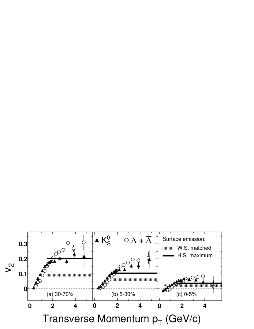
Figure 2: Comparison of $K_{S}^{0}$ and $\Lambda+\overline{\Lambda}$ $v_{2}$ with expectations from surface emission models (see text).

Figure 2 shows $v_{2}$ for $K_{S}^{0}$ and $\Lambda+\overline{\Lambda}$ from the 30–70%, 5–30%, and 0–5% centrality intervals along with calculations of $v_{2}$ from two surface emission scenarios: “W.S. matched” uses a Woods-Saxon distributions in the calculation of the nuclear overlap function and matches the energy loss to the observed suppression of neutral pion production [Jia02] while “H.S. maximum” uses an analytic function representing pure surface emission—infinite energy loss—from a hard sphere overlap geometry [Vol03]. The models are not in good agreement with our measurements. We do not, however, rule out the surface emission scenario for $p_{T}$ above 4.5 GeV/c. We also note that for $p_{T}$ from 1.5–4.5 GeV/c, it may be that kaons are produced predominantly from hard processes in a surface volume while (anti-)lambdas in the same range are produced by soft processes. The magnitude of the kaon $v_{2}$ in this region, however, is much larger than would be expected from the surface emission model with a realistic nuclear overlap density. Stronger conclusions on this point can be drawn from a larger data sample and more extensive studies of possible non-flow contributions to identified particle $v_{2}$.

In the case that particles are produced from hard processes—either near the surface or throughout the entire volume—their spectra are expected to be well represented by a power-law function [Alb90]. In Section 3 we use the power-law function

$$\frac{d^{3}n}{dp^{3}}\sim C(1+\frac{p_{T}}{p_{0}})^{-\alpha}$$ (5)

to parameterize the hard part of the $K_{S}^{0}$ and $\Lambda+\overline{\Lambda}$ spectrum.

3 Transverse Momentum Regimes

In what follows, we study the two component nature of the $K_{S}^{0}$ and $\Lambda+\overline{\Lambda}$ $p_{T}$ spectra. We seek to delineate the boundary between the soft and hard region of the spectra.

In Reference [Sor03] we stressed the effectiveness of the combination of $R_{CP}$ and $v_{2}$ for mapping out the transition between the region dominated by soft processes and the region dominated by hard processes. More detailed calculations making use of these ideas in Reference [HN03] are in relatively good agreement with the available data. We use hydrodynamical model inspired blast wave functions and pQCD motivated power-law functions to fit the $K_{S}^{0}$ and $\Lambda+\overline{\Lambda}$ spectra with the intention of extracting the value of $p_{T}$ where the soft-to-hard crossover occurs. Figure 3 shows blast wave and power-law fits to the $K_{S}^{0}$ and $\Lambda+\overline{\Lambda}$ spectra for three centrality intervals. The fit parameters are listed in Table 1.

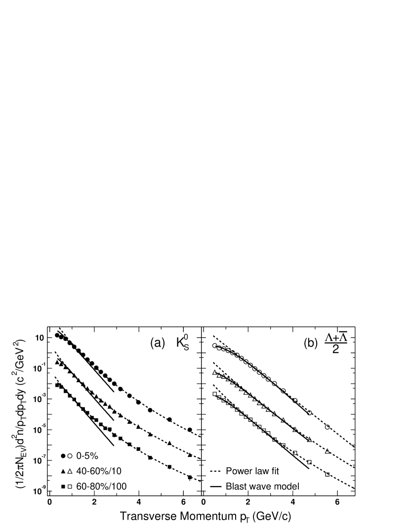
Figure 3: Blast wave and power-law fits to the $K_{S}^{0}$ and $\Lambda+\overline{\Lambda}$ spectra. Fitting parameters are listed in Table 1.

Fit	$K_{S}^{0}$			$\Lambda(\overline{\Lambda})$
Parameters	0–5%	40–60%	60–80%	0–5%	40–60%	60–80%
$C$	330.11	3.6785	0.0829	40.914	0.9832	0.0424
$p_{0}$ (GeV/c)	3.280	2.786	2.717	2.12e+5	10.38	5.691
$\alpha$	16.43	13.96	13.41	5.58e+5	34.25	21.91
$T$ (MeV)	140.7	179.1	175.5	136.3	258.7	223.2
$\rho_{0}$	0.686	0.499	0.489	0.866	0.499	0.412

Table 1: Fitting parameters for power-law (first three rows) and blast wave (last two rows) parameterizations of the $K_{S}^{0}$ and $\Lambda+\overline{\Lambda}$ spectra.

Radial flow, as established in hydrodynamical models for example, can lead to a mass dependence in the soft-to-hard $p_{T}$ crossover $p_{T,cross}$. Reference [HN03] uses the $p_{T}$ where the yields from hard and soft production processes become equivalent to define $p_{T,cross}$. Using hydrodynamic model calculations for the soft contribution, and a pQCD parton model—incorporating energy loss, gluon shadowing, and initial state rescattering—for the hard component, they calculate $p_{T,cross}=1.8$, 2.7, and 3.7 GeV/c for pions, kaons, and protons respectively. From our blast-wave and power-law fits, however, judging by the applicability of the fit functions we find that $p_{T,cross}$ for kaons in central events is closer to 1.8 GeV/c, and consistent with the pion $p_{T,cross}$ apparent in the pion spectrum measured by PHENIX [Adl03d]. Given the $p_{T}$ reach of our measurements it’s difficult to determine $p_{T,cross}$ for lambdas from spectra fits alone. We can, however, conclude that the lambda $p_{T,cross}$ is greater than 3 GeV/c: within a range that would be consistent with the proton $p_{T,cross}$ quoted in Reference [HN03].

Figure 4: The $R_{CP}$ of $K_{S}^{0}$ and $\Lambda+\overline{\Lambda}$ with blast wave curves extracted from fits to the particles spectra.

The $p_{T}$ where the $\Lambda+\overline{\Lambda}$ $R_{CP}$ (0–5%/60–80%) begins to decrease in Figure 4 (bottom panel) provides clearer evidence for the cross-over and suggest that for (anti-)lambdas $p_{T,cross}\sim 3.5$ GeV/c. We note, however, that the blast wave fits to the $\Lambda+\overline{\Lambda}$ spectra for the 0–5% and 40–60% centrality intervals are in good agreement throughout the fit range so that we cannot exclude the possibility that the blast wave parameterization describes lambda production well throughout the measured $p_{T}$. This is also apparent in the blast wave curves for $R_{CP}$ using those same centralities (the top panel of Figure 4). To determine whether or not this indicates that the assumptions of the hydrodynamical models are valid from 0–60% centrality but break down in the 80–100% interval will require further study.

The similarity of the $p_{T,cross}$ for pions and kaons may indicate that the number of quarks rather than the mass of the hadron provides the relevant scale for the transition between regions of predominantly soft and predominantly hard production processes. This empirical observation is consistent with a picture where at intermediate $p_{T}$, hadronization occurs through the coalescence of co-moving partons. The recent observation that $R_{CP}$ for the $\phi$ meson (m=1.019 GeV/c²) is closer to the pion and kaon $R_{CP}$ than the proton or lambda $R_{CP}$ [MY03] supports this picture.

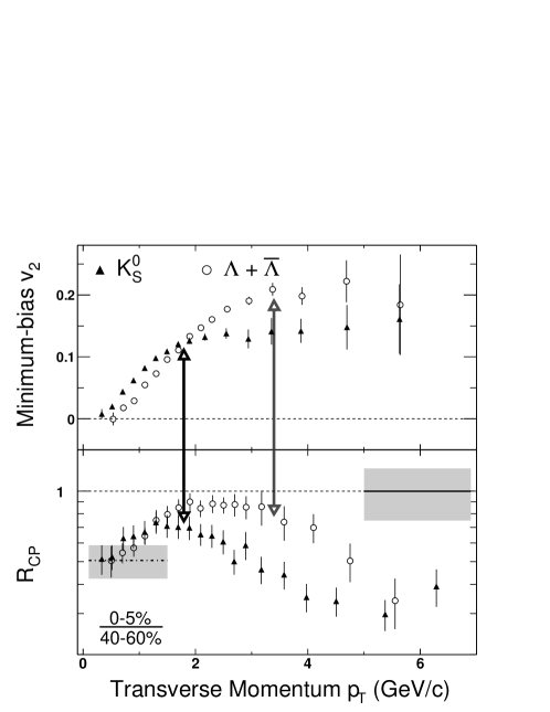
Figure 5: The $v_{2}$ and $R_{CP}$ of $K_{S}^{0}$ and $\Lambda+\overline{\Lambda}$. The vertical lines emphasize the correlation between the saturation of $v_{2}$ and the decline of $R_{CP}$.

To emphasize the correlation between the behavior of identified particle $v_{2}$ and identified particle $R_{CP}$ we plot $v_{2}$ and $R_{CP}$ together in Figure 5. Although $R_{CP}$ depends only on the yield in the central and peripheral bins, and the $v_{2}$ in Figure 5 is from a minimum-bias centrality interval, the two parameters may still be intimately related. Differential elliptic flow $v_{2}(p_{T})$ measures the difference between the $p_{T}$ spectrum of particles emitted in the direction of the reaction plane (in-plane) to that of particles emitted perpendicular the reaction plane (out-of-plane). In hydrodynamic models, we expect the pressure gradient to be larger in the in-plane direction than the out-of-plane direction. Since the average pressure gradient in central collisions is expected to be larger than in peripheral collisions in a the hydrodynamical picture the ratio $R_{CP}$ and $v_{2}$ should have a similar $p_{T}$ and particle-type dependencies. Coalescence or recombination models should also give a similar correlation between $v_{2}$ and $R_{CP}$. Both measures reflect relative probabilities for forming hadrons: The probabilities depend on the phase-space density of partons, and the phase-space density varies with centrality and azimuthal angle. In Appendix 7 we introduce a formalism more suited to studying the centrality dependence of particle yields in heavy-ion collisions across a broad $p_{T}$ range and for a variety of system sizes.

4 Initial State Effects

Nuclear enhancement of hadron yields (relative to number-of-binary-collisions scaling) for lower beam energies has been observed at intermediate $p_{T}$ in p+A collisions—with a larger enhancement for baryons than mesons [Str92]. The empirical observation of an enhancement in the scaled yield is known as the Cronin effect [Cro73, Ant79]. The Cronin effect is generally attributed to multiple scatterings between the projectile partons and the cold nuclear matter in the target [Acc02]. The ratio of the scaled yields in d+Au and p+p collisions $R_{dAu}$ has been measured for neutral pions [Adl03c] and inclusive charged hadrons at RHIC [Ada03a, Bac03a, Adl03c, Ars03]. At intermediate $p_{T}$, the neutral pion $R_{dAu}$ is consistent with one (no Cronin effect) or a small enhancement. The inclusive charged hadron $R_{dAu}$ shows an enhancement of roughly 35% however, indicating the presence of a particle-type dependent Cronin effect at RHIC energy. The existence of an enhancement has not been established for kaons, lambdas, or antilambdas, but the Cronin effect cannot be ruled out as the origin of the dependence of $R_{CP}$ on particle type.

Theoretical calculations, such as those involving initial parton scatterings off cold nuclear matter (e.g. [LP83]), don’t reproduce the particle-type dependence of the enhancement factor observed in p+A collisions. The inadequate particle dependence in these calculations may arise from the fact that these models only deal with initial parton scatterings while the observed hadrons are formed at the late stage of the collision. It is argued in Reference [AG03], that the fragmentation process can distort the features of the parton level Cronin effect. As such, the strong particle-type dependence in $R_{p(d)A}$ may indicate a nuclear modification of the parton fragmentation into baryons and mesons or alternatively, the presence in p(d)+A collisions of a multi-parton particle formation mechanism such as coalescence [GKL03a] or recombination [FMN03a]. These mechanisms are beyond the framework of many existing theoretical models for the Cronin effect.

5 Hadronization of Dense Matter

The varied initial conditions in heavy-ion collisions may provide important phenomenological clues to the nature of hadron formation—particularly baryon formation. Observing how the presence of dense nuclear matter influences hadronization will almost certainly help clarify by what processes three quarks can come together to form a baryon.

Modification of the fragmentation functions $D_{a\rightarrow h}(z)$ has been offered as a strategy to account for the influence of the surrounding matter on the fragmentation process [GW00, WG01]. When this strategy leads to a rescaling of $z$ it should affect all hadrons in a similar way [FMN03a]—a behavior that is inconsistent with the measurements presented in this thesis. To account for species dependence observed in $v_{2}$ and $R_{CP}$ a new understanding of hadronization may be necessary. In addition, we note that in the complex and highly interacting systems created in heavy-ion collisions the assumption of factorization implicit in Equation 4 may no longer be valid.

Although the observables of heavy-ion collisions—$R_{CP}$, particle ratios, and $v_{2}$ for example—and their variation with particle-type challenge current theoretical models, they also hint at possible resolutions.

We note for example, that the absence of a significant suppression with respect to binary scaling of the $\Lambda+\overline{\Lambda}$ yield at intermediate $p_{T}$ in central Au+Au collisions may indicate the presence of dynamics beyond parton energy loss and standard fragmentation. The larger $\Lambda+\overline{\Lambda}$ $R_{CP}$ at intermediate $p_{T}$ means that the (anti-)lambda yield increases with the parton density of the collision fireball much faster than the meson yield. The rate of increase of the proton yield [Adl03e] and the multi-strange baryon yield ($\Xi+\overline{\Xi}$) [Lon03] are found to be similar to that of (anti-)lambda. In addition, at intermediate $p_{T}$, the centrality dependence of the $\phi$-meson production is more similar to that of kaons than (anti-)lambdas [MY03]. Stronger dependence on parton density for baryon production is naturally expected from multi-parton production mechanisms such as gluon junctions [VG99], quark coalescence [MV03], or recombination [FMN03b].

As discussed in Section 3, it is apparently the number of constituent quarks in a hadron that predominantly determines the characteristics of it’s spectra at intermediate $p_{T}$. Figure 6 shows $v_{2}$ of $K_{S}^{0}$ and $\Lambda+\overline{\Lambda}$ as a function of $p_{T}$, where the $v_{2}$ and $p_{T}$ values have been scaled by the number of constituent quarks (n). While $v_{2}$ is significantly different for $K_{S}^{0}$ and $\Lambda+\overline{\Lambda}$, within errors, $v_{2}$/n vs $p_{T}$/n is the same for both species above $p_{T}$/n $\sim 0.8$ GeV/c. This behavior is consistent with a scenario where hadrons at intermediate $p_{T}$ are formed from bulk partonic matter by coalescence of co-moving quarks: in this case $v_{2}/$n vs $p_{T}/$n reveals the momentum space azimuthal anisotropy that partons develop from the collision ellipsoid, e.g. Reference [MV03]. Hadronization by coalescence and the large partonic anisotropy subsequently inferred from our empirical observations would both argue strongly for the existence of a strongly interacting early partonic stage.

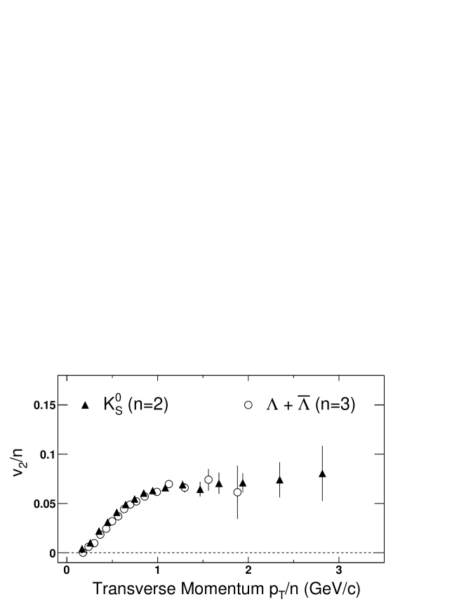
Figure 6: The $v_{2}$ parameter for $K_{S}^{0}$ and $\Lambda+\overline{\Lambda}$ scaled by the number of constituent quarks (n) and plotted versus $p_{T}/$n.

The suggestive scaling behavior if Figure 6 can be tested by including measurements of $v_{2}$ for other identified particles that extend into the intermediate $p_{T}$ region. Figure 7 shows $v_{2}/$n versus $p_{T}/$n for all identified particles currently available from RHIC experiments [Esu03, CS03]. At low $p_{T}$ ($p_{T}<1$ GeV/c), where hydrodynamic calculations were already seen to reproduce the measured $v_{2}$ well, and at $p_{T}>6$ GeV/c, the signatures of coalescence are not expected to be prominent. The deviation of the scaled pion $v_{2}$ may prove to be problematic or it may just reflect the break-down of coalescence at low $p_{T}$. Otherwise, the results in Figure 7 are consistent with the expectations of constituent-quark-number scaling and provide strong evidence for coalescence and the existence of a quark-gluon plasma in the early stage of the collision system.

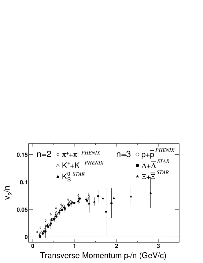
Figure 7: The $v_{2}$ parameter for $K_{S}^{0}$ and $\Lambda+\overline{\Lambda}$ scaled by the number of constituent quarks (n) and plotted versus $p_{T}/$n.

For n$\times p_{T,hard}$, where $p_{T,hard}$ is a momentum for which the spectra of the underlying partons follows a power-law, the yield of hadrons from coalescence of n quarks will no longer dominate the yield of hadrons from fragmentation of partons with momentum $p_{T,hard}/z$. Based on this picture, we would expect the $v_{2}$ of all hadrons at high $p_{T}$ ($p_{T}>6$) to take on the unscaled value of the parton $v_{2}$. Assuming the $v_{2}/$n values from Figure 7 reflect the parton $v_{2}$ we would conclude that at high $p_{T}$ (where we expect $v_{2}^{meson}=v_{2}^{baryon}=v_{2}^{quark}$), $v_{2}$ of all light-flavored particles (particles having only u, d, or s constituent quarks) will take on the same value $v_{2,hard}\sim 0.07$. This assumes a saturated parton $v_{2}$ at high $p_{T}$: an assumption that is consistent with expectations from transport [MG02], and surface emission [Shu02] models.

6 Conclusions

In summary, we have reported the measurement of $v_{2}$ and $R_{CP}$ up to $p_{T}$ of $6.0$ GeV/c for kaons and $\Lambda+\overline{\Lambda}$ from Au+Au collisions at $\sqrt{s_{{}_{NN}}}=200$ GeV. At low $p_{T}$, hydrodynamic model calculations agree well with $v_{2}$ for $K_{S}^{0}$ and $\Lambda+\overline{\Lambda}$. At intermediate $p_{T}$, however, hydrodynamics no longer describes the particle production well. For $K_{S}^{0}$, $v_{2}$ saturates earlier and at a lower value than for $\Lambda+\overline{\Lambda}$. In addition, $R_{CP}$ shows that the kaon yield in central collisions is suppressed more than the (anti-)lambda yield. At intermediate $p_{T}$, the $\Lambda+\overline{\Lambda}$ yield in central Au+Au collisions is close to expectations from binary scaling of peripheral Au+Au collisions. At high $p_{T}$, the $R_{CP}$ of $K_{S}^{0}$, $\Lambda+\overline{\Lambda}$ and charged hadrons are approaching the same value. The measured features in the kaon and (anti-)lambda $v_{2}$ and $R_{CP}$ may indicate the presence of dynamics beyond the framework of parton energy loss followed by fragmentation. The particle- and $p_{T}$-dependence of $v_{2}$ and $R_{CP}$, particularly at intermediate $p_{T}$, provides a unique means to investigate the anisotropy and hadronization of the bulk dense matter formed in nucleus-nucleus collisions at RHIC.

In Au+Au collisions that copiously populate phase space, it would be naive to expect a single parton description of hadronization to remain valid. Our measurements verify that multi-parton dynamics significantly alter production mechanisms: giving rise to a number-of-constituent-quark dependence for particle spectra, $R_{CP}$, and $v_{2}$ at intermediate $p_{T}$. From the mass dependence of $v_{2}$ at low $p_{T}$ and the partonic $v_{2}$ inferred from the scaled $v_{2}$ at intermediate $p_{T}$ it appears that the existence of a thermalized partonic state at RHIC is not just likely but perhaps unavoidable.

7 Future Directions

The future direction of our studies at RHIC are clear: verification of the creation of a QGP, then characterization of the QGP. The measurement of identified particle $v_{2}$ and $R_{CP}$ will play a prominent role in both of these endeavors. The full implication of the measurements presented in this thesis will become clearer when $v_{2}$ and $R_{CP}$ have been measured well into the hard region ($p_{T}\approx 8$ GeV/c) for $\pi^{0}$, $K_{S}^{0}$, and $\phi$ mesons and for $p$, $\Lambda$, $\Xi$, and $\Omega$ baryons. Several of these measurements are already available and most of the others will become available in the near future. The measurements already made argue strongly for the existence of a thermalized partonic state that at least partly hadronizes by coalescence. With the larger data sets collected during future RHIC runs $v_{2}$ should be measured for identified particles using a cumulant analysis. The cumulant analysis can easily be adapted for statistically identified particles when only one particle candidate in a given $p_{T}$ interval is considered from each event.

Once a suite of identified meson and baryon measurements has been made to sufficiently high $p_{T}$, the first priority should be to conduct a system-size scan. RHIC is already operating at its top energy for Au+Au collisions and running with lower energy will drastically reduce high $p_{T}$ particle yields—essentially eliminating several of our most promising QGP signatures. Instead, it will be more fruitful to study collisions with fewer participants. This will provide three exciting opportunities: A chance to search for a region where the QGP state is turned on or off, a chance to run at even higher energy with the existing RHIC facility (Si+Si top energy would be $\sqrt{s_{{}_{NN}}}=250$ GeV) and the chance to search for rare/exotic states (i.e. glue-balls, penta-quarks, etc.) in collisions that generate less combinatorial background. The reduction in the combinatorial background will benefit many identified particle measurements. Cu+Cu collisions may be preferable since they should still allow reliable measurements of $v_{2}$ while probing smaller system sizes.

Chapter 5 Collision Geometry and the Source Eccentricity

Here we provide information about the geometry and coordinate systems of relativistic heavy-ion collisions.

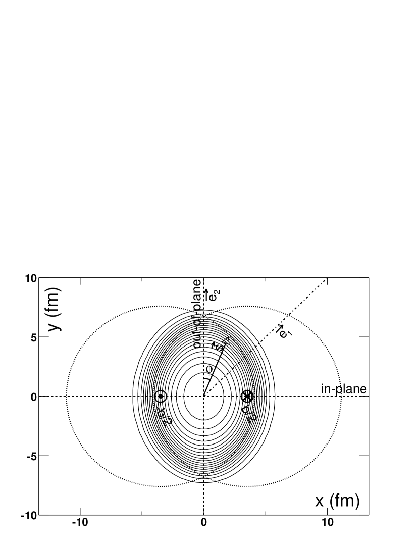
Figure 1: Coordinate system for the transverse plane in heavy-ion collisions. Contours of the overlap density are also shown. Here $\phi$ is the azimuthal angle with respect to the $y$-axis. Also shown are generalized coordinates $\vec{e_{1}}$ and $\vec{e_{2}}$ used to calculate the fourth-harmonic eccentricity where the ($y$-)$\vec{e_{2}}$-axis is the only uniquely defined direction in the transverse plane.

Figure 1 gives the coordinates in the azimuthal plane of the collisions. The beam direction ($z$-axis) is in or out of the page as indicated by the $\otimes$ or $\odot$ respectively. The ($y$-)$\vec{e_{2}}$-axis is uniquely defined (using the right-hand-rule) by the collision axis and the directions of the colliding beams. When calculating $v_{2}=\langle\cos(2\phi)\rangle$, $\phi$ is defined with respect to the reaction plane (the $x$-axis). For our eccentricity calculations we will define $\phi$ with respect to the $y$-axis. In this way, $v_{2}$ and the $2^{nd}$-harmonic eccentricity will have the same sign.

The density of Au nucleus is represented by a Woods-Saxon distribution,

$$\rho_{A}=\rho_{0}\frac{1}{1+\exp(\frac{r-R_{A}}{\xi})}$$ (1)

where $r=\sqrt{s^{2}+z^{2}}$, $R_{A}=1.12\times A^{1/3}$, with $\rho_{0}=0.159$ GeV/fm³ and $\xi=0.535$ fm. The thickness function of nucleus $A$ ($T_{A}$) is the nuclear density integrated over the $z$ direction: $T_{A}(\vec{s})=\int dz\rho_{A}(a,\vec{s})$. The density of nucleons participating in the collision (wounded nucleons) is given by:

$$n_{part}(x,y)=T_{A}\times(1-e^{-T_{B}\sigma_{NN}})+T_{B}\times(1-e^{-T_{A}\sigma_{NN}}),$$ (2)

where for collisions at $\sqrt{s_{{}_{NN}}}=200$ GeV we use $\sigma_{NN}\approx 42$. The density of binary nucleon-nucleon collisions is taken as: $n_{bin}(x,y)=\sigma_{NN}\times T_{A}\times T_{B}$. In the plots that follow, we use $n_{part}$ as the density in the overlap region.

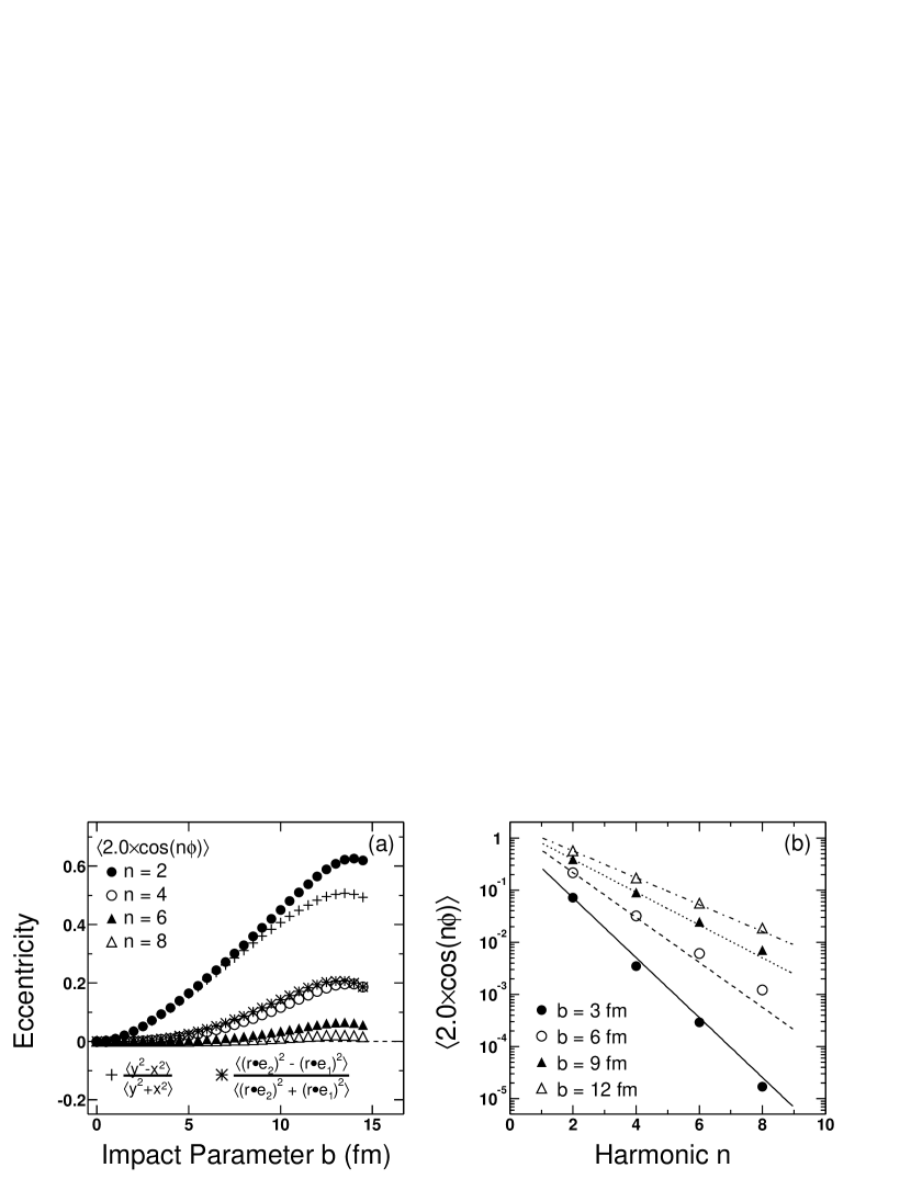
Figure 2: Left: Analytic calculations of the even n$th$-harmonic eccentricities versus impact parameter. Right: Relative magnitudes of harmonics for various impact parameters. For more central collisions the higher harmonics fall off more quickly.

To better understand the initial spatial asymmetry of the collision regions in Figure 2 we show calculations of eccentricities defined for even harmonics (the odd harmonic eccentricities are all zero). The most commonly used definition of the second harmonic eccentricity is $\epsilon_{2}=\langle y^{2}-x^{2}\rangle/\langle y^{2}+x^{2}\rangle$. In the figure we also include calculations of eccentricities from $2\langle\cos(n\phi)\rangle$ and a calculation of the $4^{th}$-harmonic eccentricity using the appropriate coordinate system as shown in Figure 1. We note that the magnitude of higher harmonic eccentricities falls off more quickly in central collisions than peripheral collisions (panel b). For peripheral collisions the higher harmonics are appreciably larger. The different methods for calculating the eccentricity do not yield the same result. In Figure 3 we show the eccentricity from the more standard calculation. We also show the ratio of the $2^{nd}$- and $4^{th}$-harmonic eccentricities versus impact parameter (panel b).

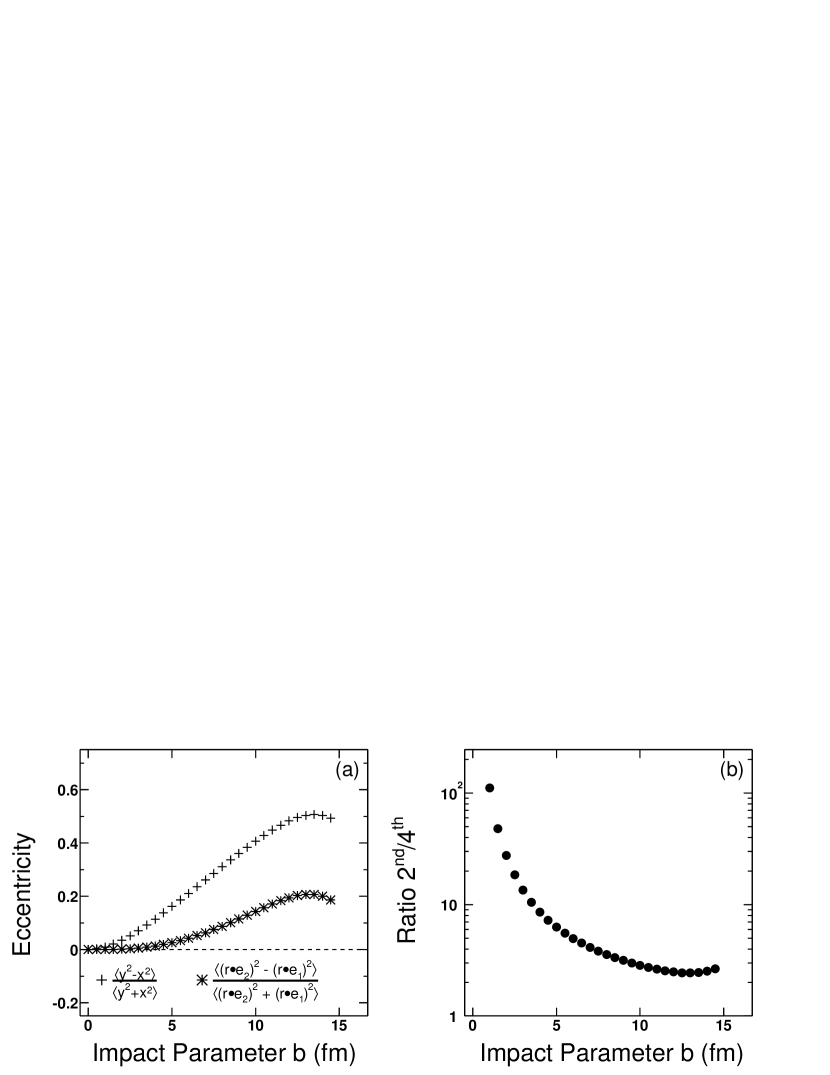
Figure 3: Left: Analytic calculations of the $2^{nd}$-harmonic and $4^{th}$-harmonic eccentricities. Right: The ratio of the second and fourth harmonic eccentricities.

In Figure 4 (a) we plot profiles (along the x and y axis) of the overlap density for the impact parameters listed in panel b. In Figure 4 (b) we plot the gradient of the profiles in panel a. In a hydrodynamical picture—once a system has thermalized—the density changes will generate pressure gradients that drive the flow of matter and induce collective motion. We note that Figure 4 (b) suggests that the greatest initial pressure gradients will be found in the in-plane direction of collisions having impact parameter $b=6$ fm. This impact parameter corresponds roughly to collisions within the 10–20% centrality interval.

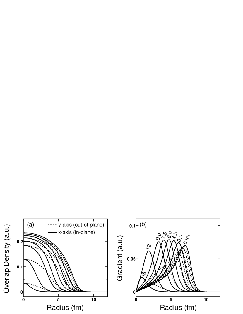
Figure 4: Left: Collision overlap densities calculated for various impact parameters (listed in panel b) and using a Woods-Saxon nuclear density profile and a wounded nucleon model. Right: The gradients of the density profiles in panel a. We take the magnitude of the gradient to estimate of the initial pressures in the system.

In Figure 5 we show the geometries corresponding to the centrality intervals used in our $v_{2}$ measurements. The mean eccentricities and impact parameters in this figure were calculated as in Reference [Adl02c].

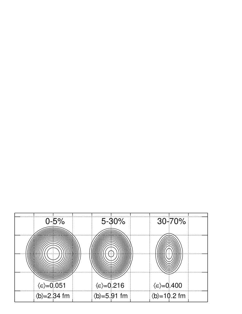
Figure 5: Overlap densities, mean eccentricities, and mean impact parameters for the centrality intervals used for our $v_{2}$ analysis.

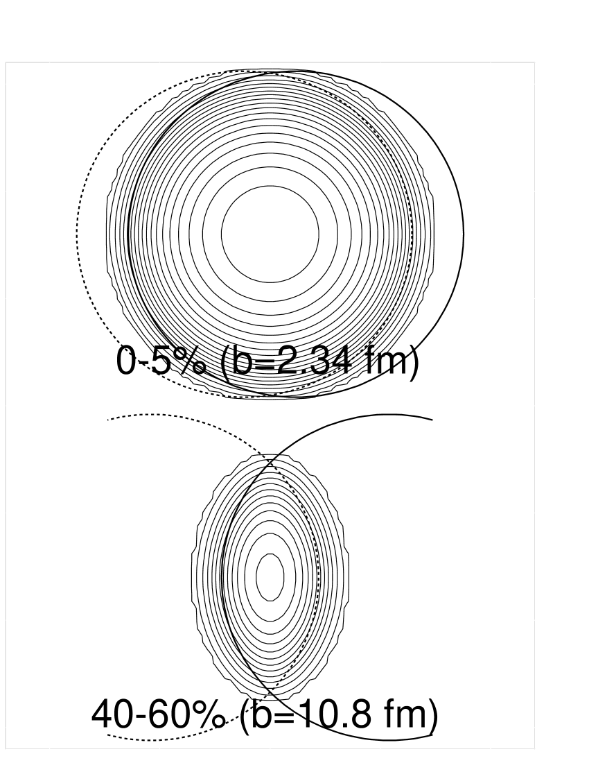
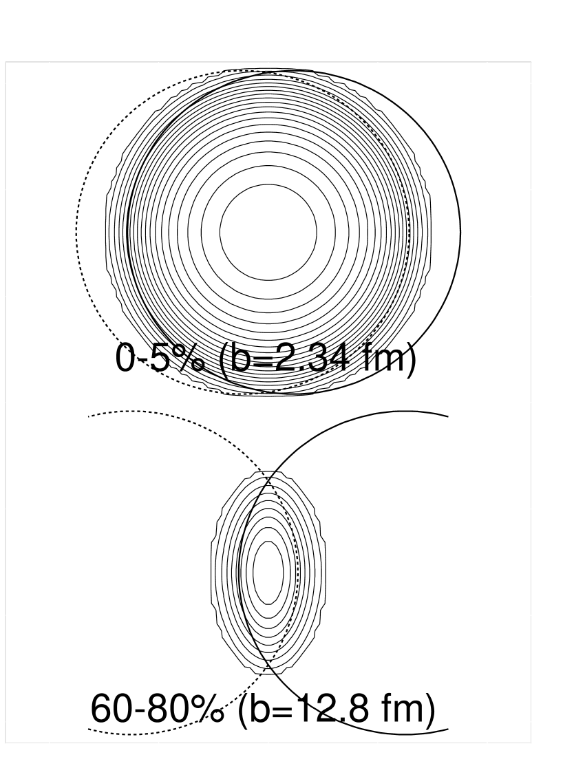
Figure 6: Configurations for the collision centrality intervals used to calculate $R_{CP}$.

In Figure 6 we show the geometry of the centrality intervals used in the calculation of $R_{CP}$.

Chapter 6 Kinematic Variables

The azimuthal components of a particles momentum $p_{x}$ and $p_{y}$ are used to define its transverse momentum,

$$p_{T}\equiv\sqrt{p_{x}^{2}+p_{y}^{2}}.$$ (1)

The transverse mass/energy of a particle having mass $m_{0}$ is

$$m_{T}\equiv\sqrt{p_{T}^{2}+m_{0}^{2}},$$ (2)

so that the transverse kinetic energy of the particle is $m_{T}-m_{0}$. The transverse kinetic energy is commonly used in place of $p_{T}$.

In the lab frame, the azimuthal angle of a particles momentum is simply $\phi_{lab}=\tan^{-1}(p_{y}/p_{x})$. When the reaction plane can be measured the azimuthal angle can be measured with respect to the transverse angle of the reaction plane $\Psi_{RP}$:

$$\phi=\phi_{lab}-\Psi_{RP}.$$ (3)

This is the $\phi$ shown in Figure 1 where the reaction plane is aligned with the $x$-axis.

With the transverse coordinates defined all that remains is to define a longitudinal variable. The rapidity $y$ is defined as

$$y\equiv\frac{1}{2}\ln\left(\frac{E+p_{z}}{E-p_{z}}\right)$$ (4)

and is boost invariant. In the case that the momentum of a particle is known but not its energy—typically because it’s mass is unknown—then the pseudo-rapidity $\eta=-\ln\tan\left(\cos^{-1}(p_{z}/p)/2\right)$ can be used. For $p\gg m$, $\eta\approx y$.

The differential cross-section for particle production, is found by counting the number of particles $d^{3}n$ produced in a phase space element. It’s advantageous to define the phase-space element to be Lorentz invariant. The usual choice is the element $dp_{x}dp_{y}dp_{z}/E$, so that the invariant cross-section is

$$E\frac{d^{3}n}{dp^{3}}=\frac{d^{3}n}{p_{T}dp_{T}d\phi dy},$$ (5)

where we’ve expressed the cross-section in terms of the variables defined previously.

Chapter 7 An Improved Formalism for Studying the System Size Dependence of Nucleus-Nucleus Collisions

Up to now the centrality dependence of particle yields in heavy-ion collision has primarily been studied either by plotting the spectra from different centralities in the same panel or by forming the ratio

$$R_{CP}(p_{T})=\frac{\left[dn/\left(\mathrm{N_{binary}}dp_{T}\right)\right]^{\mathrm{central}}}{\left[dn/\left(\mathrm{N_{binary}}dp_{T}\right)\right]^{\mathrm{peripheral}}}.$$ (1)

This ratio is formed in order to test how different high $p_{T}$ particle production in central collisions is from peripheral collisions where yields are expected to scale by the number of binary collisions. Here we suggest another formalism that we believe is better suited to the study of the centrality dependence of particle production in a variety of heavy-ion collision systems and across the entire $p_{T}$ range.

Particle yields scale predominantly with the number of participating nucleons $\mathrm{N_{part}}$, not $\mathrm{N_{binary}}$ and $\mathrm{N_{part}}$ is less model dependent than $\mathrm{N_{binary}}$. For this reason we choose to consider the yield of a particle $Y$ from collisions with impact parameter $b$ scaled by $\mathrm{N_{part}}$:

$$y(b)\equiv Y(b)/\mathrm{N_{part}}.$$ (2)

We can write $y(b)$ in terms of a Taylor expansion around a given impact parameter $b_{0}$:

$$y(b)=y(b_{0})\left(1+\frac{1}{y(b_{0})}\frac{\partial y}{\partial b}(b-b_{0})+\frac{1}{2y(b_{0})}\frac{\partial^{2}y}{\partial b^{2}}(b-b_{0})^{2}+\dots\right).$$ (3)

We label the terms $s_{1}=\frac{1}{y(b_{0})}\frac{\partial y}{\partial b}$, $s_{2}=\frac{1}{2y(b_{0})}\frac{\partial^{2}y}{\partial b^{2}}$, etc. so that $s_{n}=\frac{1}{(n-1)!y(b_{0})}\frac{\partial^{n}y}{\partial b^{n}}$. In this case if the yield scales with $\mathrm{N_{part}}$ then $s_{n}=0$ for all $n$. The term $s_{1}$ represents the linear dependence of $y(b)$ and $s_{2}$ represents the quadratic dependence.

These measures have several benefits over the scaled ratio $R_{CP}$. First we note that if one of the centrality parameters $s_{n}$ is dominant then coalescence scaling would give $s_{n}^{meson}(p_{T})=2\times s_{n}^{quark}(p_{T}/2)$ and $s_{n}^{baryon}(p_{T})=3\times s_{n}^{quark}(p_{T}/3)$. Even if several parameters must be taken into account trivial scaling rules relating meson and baryon $s$ parameters can still be attained. Second, we can easily define a minimum-bias $s_{n}$ measurement or an $s_{n}$ measurement within a given centrality so that the centrality dependence at different intervals and for different systems can be more easily compared. For example, we can expand $y(b)$ about $b_{0}=b_{max}/2.0$ and calculate the minimum-bias $s_{1}=\frac{12\langle b-b_{0}\rangle}{b_{max}^{2}}$ (where the scaled yield $y$ has been used to calculate the mean). These variables may be particularly valuable for studying changes to the systematic variation of the yield with system size. One would hope to see a notable change in the $s$ parameters as the system size increases to a size necessary to form a QGP.

A correction to the $s_{n}$ variables can be introduced to account for the impact parameter resolution.

Chapter 8 The STAR Collaboration

J. Adams³, C. Adler¹¹, Z. Ahammed²⁴, C. Allgower¹², J. Amonett¹⁴, B.D. Anderson¹⁴, M. Anderson⁵, D. Arkhipkin¹⁰, G.S. Averichev⁹, J. Balewski¹², O. Barannikova^9,24, L.S. Barnby¹⁴, J. Baudot¹³, S. Bekele²¹, V.V. Belaga⁹, R. Bellwied³³, J. Berger¹¹, H. Bichsel³², A. Billmeier³³, L.C. Bland², C.O. Blyth³, B.E. Bonner²⁵, M. Botje²⁰, A. Boucham²⁸, A. Brandin¹⁸, A. Bravar², R.V. Cadman¹, X.Z. Cai²⁷, H. Caines³⁵, M. Calderón de la Barca Sánchez², A. Cardenas²⁴, J. Carroll¹⁵, J. Castillo¹⁵, M. Castro³³, D. Cebra⁵, P. Chaloupka²¹, S. Chattopadhyay³³, Y. Chen⁶, S.P. Chernenko⁹, M. Cherney⁸, A. Chikanian³⁵, B. Choi³⁰, W. Christie², J.P. Coffin¹³, T.M. Cormier³³, M. Mora Corral¹⁶, J.G. Cramer³², H.J. Crawford⁴, A.A. Derevschikov²³, L. Didenko², T. Dietel¹¹, J.E. Draper⁵, V.B. Dunin⁹, J.C. Dunlop³⁵, V. Eckardt¹⁶, L.G. Efimov⁹, V. Emelianov¹⁸, J. Engelage⁴, G. Eppley²⁵, B. Erazmus²⁸, P. Fachini², V. Faine², J. Faivre¹³, R. Fatemi¹², K. Filimonov¹⁵, E. Finch³⁵, Y. Fisyak², D. Flierl¹¹, K.J. Foley², J. Fu^15,34, C.A. Gagliardi²⁹, N. Gagunashvili⁹, J. Gans³⁵, L. Gaudichet²⁸, M. Germain¹³, F. Geurts²⁵, V. Ghazikhanian⁶, O. Grachov³³, M. Guedon¹³, S.M. Guertin⁶, E. Gushin¹⁸, T.D. Gutierrez⁵, T.J. Hallman², D. Hardtke¹⁵, J.W. Harris³⁵, M. Heinz³⁵, T.W. Henry²⁹, S. Heppelmann²², T. Herston²⁴, B. Hippolyte¹³, A. Hirsch²⁴, E. Hjort¹⁵, G.W. Hoffmann³⁰, M. Horsley³⁵, H.Z. Huang⁶, T.J. Humanic²¹, G. Igo⁶, A. Ishihara³⁰, P. Jacobs¹⁵, W.W. Jacobs¹², M. Janik³¹, I. Johnson¹⁵, P.G. Jones³, E.G. Judd⁴, S. Kabana³⁵, M. Kaneta¹⁵, M. Kaplan⁷, D. Keane¹⁴, J. Kiryluk⁶, A. Kisiel³¹, J. Klay¹⁵, S.R. Klein¹⁵, A. Klyachko¹², T. Kollegger¹¹, A.S. Konstantinov²³, M. Kopytine¹⁴, L. Kotchenda¹⁸, A.D. Kovalenko⁹, M. Kramer¹⁹, P. Kravtsov¹⁸, K. Krueger¹, C. Kuhn¹³, A.I. Kulikov⁹, G.J. Kunde³⁵, C.L. Kunz⁷, R.Kh. Kutuev¹⁰, A.A. Kuznetsov⁹, M.A.C. Lamont³, J.M. Landgraf², S. Lange¹¹, C.P. Lansdell³⁰, B. Lasiuk³⁵, F. Laue², J. Lauret², A. Lebedev², R. Lednický⁹, V.M. Leontiev²³, M.J. LeVine², Q. Li³³, S.J. Lindenbaum¹⁹, M.A. Lisa²¹, F. Liu³⁴, L. Liu³⁴, Z. Liu³⁴, Q.J. Liu³², T. Ljubicic², W.J. Llope²⁵, H. Long⁶, R.S. Longacre², M. Lopez-Noriega²¹, W.A. Love², T. Ludlam², D. Lynn², J. Ma⁶, Y.G. Ma²⁷, D. Magestro²¹, R. Majka³⁵, S. Margetis¹⁴, C. Markert³⁵, L. Martin²⁸, J. Marx¹⁵, H.S. Matis¹⁵, Yu.A. Matulenko²³, T.S. McShane⁸, F. Meissner¹⁵, Yu. Melnick²³, A. Meschanin²³, M. Messer², M.L. Miller³⁵, Z. Milosevich⁷, N.G. Minaev²³, J. Mitchell²⁵, C.F. Moore³⁰, V. Morozov¹⁵, M.M. de Moura³³, M.G. Munhoz²⁶, J.M. Nelson³, P. Nevski², V.A. Nikitin¹⁰, L.V. Nogach²³, B. Norman¹⁴, S.B. Nurushev²³, G. Odyniec¹⁵, A. Ogawa², V. Okorokov¹⁸, M. Oldenburg¹⁶, D. Olson¹⁵, G. Paic²¹, S.U. Pandey³³, Y. Panebratsev⁹, S.Y. Panitkin², A.I. Pavlinov³³, T. Pawlak³¹, V. Perevoztchikov², W. Peryt³¹, V.A Petrov¹⁰, R. Picha⁵, M. Planinic¹², J. Pluta³¹, N. Porile²⁴, J. Porter², A.M. Poskanzer¹⁵, E. Potrebenikova⁹, D. Prindle³², C. Pruneau³³, J. Putschke¹⁶, G. Rai¹⁵, G. Rakness¹², O. Ravel²⁸, R.L. Ray³⁰, S.V. Razin^9,12, D. Reichhold²⁴, J.G. Reid³², G. Renault²⁸, F. Retiere¹⁵, A. Ridiger¹⁸, H.G. Ritter¹⁵, J.B. Roberts²⁵, O.V. Rogachevski⁹, J.L. Romero⁵, A. Rose³³, C. Roy²⁸, V. Rykov³³, I. Sakrejda¹⁵, S. Salur³⁵, J. Sandweiss³⁵, I. Savin¹⁰, J. Schambach³⁰, R.P. Scharenberg²⁴, N. Schmitz¹⁶, L.S. Schroeder¹⁵, K. Schweda¹⁵, J. Seger⁸, P. Seyboth¹⁶, E. Shahaliev⁹, K.E. Shestermanov²³, S.S. Shimanskii⁹, F. Simon¹⁶, G. Skoro⁹, N. Smirnov³⁵, R. Snellings²⁰, P. Sorensen⁶, J. Sowinski¹², H.M. Spinka¹, B. Srivastava²⁴, E.J. Stephenson¹², R. Stock¹¹, A. Stolpovsky³³, M. Strikhanov¹⁸, B. Stringfellow²⁴, C. Struck¹¹, A.A.P. Suaide³³, E. Sugarbaker²¹, C. Suire², M. Šumbera²¹, B. Surrow², T.J.M. Symons¹⁵, A. Szanto de Toledo²⁶, P. Szarwas³¹, A. Tai⁶, J. Takahashi²⁶, A.H. Tang¹⁵, D. Thein⁶, J.H. Thomas¹⁵, M. Thompson³, S. Timoshenko¹⁸, M. Tokarev⁹, M.B. Tonjes¹⁷, T.A. Trainor³², S. Trentalange⁶, R.E. Tribble²⁹, V. Trofimov¹⁸, O. Tsai⁶, T. Ullrich², D.G. Underwood¹, G. Van Buren², A.M. Vander Molen¹⁷, A.N. Vasiliev²³, S.E. Vigdor¹², S.A. Voloshin³³, M. Vznuzdaev¹⁸, F. Wang²⁴, Y. Wang³⁰, H. Ward³⁰, J.W. Watson¹⁴, R. Wells²¹, G.D. Westfall¹⁷, C. Whitten Jr. ⁶, H. Wieman¹⁵, R. Willson²¹, S.W. Wissink¹², R. Witt³⁵, J. Wood⁶, N. Xu¹⁵, Z. Xu², A.E. Yakutin²³, E. Yamamoto¹⁵, J. Yang⁶, P. Yepes²⁵, V.I. Yurevich⁹, Y.V. Zanevski⁹, I. Zborovský⁹, H. Zhang³⁵, W.M. Zhang¹⁴, R. Zoulkarneev¹⁰, J. Zoulkarneeva¹⁰, A.N. Zubarev⁹

¹Argonne National Laboratory, Argonne, Illinois 60439
²Brookhaven National Laboratory, Upton, New York 11973
³University of Birmingham, Birmingham, United Kingdom
⁴University of California, Berkeley, California 94720
⁵University of California, Davis, California 95616
⁶University of California, Los Angeles, California 90095
⁷Carnegie Mellon University, Pittsburgh, Pennsylvania 15213
⁸Creighton University, Omaha, Nebraska 68178
⁹Laboratoryfor High Energy (JINR), Dubna, Russia
¹⁰Particle Physics Laboratory (JINR), Dubna, Russia
¹¹University of Frankfurt, Frankfurt, Germany
¹²Indiana University, Bloomington, Indiana 47408
¹³Institut de Recherches Subatomiques, Strasbourg, France
¹⁴Kent State University, Kent, Ohio 44242
¹⁵LawrenceBerkeley National Laboratory, Berkeley, California 94720
¹⁶Max-Planck-Institut fuer Physik, Munich, Germany
¹⁷Michigan State University, East Lansing, Michigan 48825
¹⁸Moscow Engineering Physics Institute, Moscow Russia
¹⁹City College of New York, New York City, New York 10031
²⁰NIKHEF, Amsterdam, The Netherlands
²¹Ohio State University, Columbus, Ohio 43210
²²Pennsylvania State University, University Park, Pennsylvania 16802
²³Institute of High Energy Physics, Protvino, Russia
²⁴Purdue University, West Lafayette, Indiana 47907
²⁵Rice University, Houston, Texas 77251
²⁶Universidade de Sao Paulo, Sao Paulo, Brazil
²⁷Shanghai Institute of Nuclear Research, Shanghai 201800, P.R. China
²⁸SUBATECH, Nantes, France
²⁹Texas A&M University, College Station, Texas 77843
³⁰University of Texas, Austin, Texas 78712
³¹Warsaw University of Technology, Warsaw, Poland
³²University of Washington, Seattle, Washington 98195
³³Wayne State University, Detroit, Michigan 48201
³⁴Institute of Particle Physics, CCNU (HZNU), Wuhan, 430079 China
³⁵Yale University, New Haven, Connecticut 06520

References

- [Acc02] A. Accardi. “Cronin Effect in Proton Nucleus Collisions: A Survey of Theoretical Models.” hep-ph/0212148, 2002.
- [Ack01] K. H. Ackermann et al. “Elliptic Flow in Au + Au Collisions at GeV.” Phys. Rev. Lett., 86:402–407, 2001.
- [Ack03] K. H. Ackermann et al. “The STAR Detector.” Nucl. Instr. Meth., A499:624, 2003.
- [Ada02] D. Adamova et al. “New Results from CERES.” Nucl. Phys., A698:253–260, 2002.
- [Ada03a] J. Adams et al. “Evidence from d + Au Measurements for Final-State Suppression of High Hadrons in Au + Au Collisions at RHIC.” Phys. Rev. Lett., 91:072304, 2003.
- [Ada03b] J. Adams et al. “Transverse Momentum and Collision Energy Dependence of High Hadron Suppression in Au + Au Collisions at Ultrarelativistic Energies.” nucl-ex/0305015, 2003.
- [Adc01] K. Adcox et al. “Centrality Dependence of Charged Particle Multiplicity in Au Au Collisions at GeV.” Phys. Rev. Lett., 86:3500–3505, 2001.
- [Adl01] C. Adler et al. “Identified Particle Elliptic Flow in Au + Au Collisions at GeV.” Phys. Rev. Lett., 87:182301, 2001.
- [Adl02a] C. Adler et al. “Azimuthal Anisotropy of and Production at Mid-rapidity from Au + Au Collisions at GeV.” Phys. Rev. Lett., 89:132301, 2002.
- [Adl02b] C. Adler et al. “Centrality Dependence of High Hadron Suppression in Au + Au Collisions at GeV.” Phys. Rev. Lett., 89:202301, 2002.
- [Adl02c] C. Adler et al. “Elliptic Flow from Two- and Four-particle Correlations in Au + Au Collisions at GeV.” Phys. Rev., C66:034904, 2002.
- [Adl02d] C. Adler et al. “Kaon Production and Kaon to Pion Ratio in Au + Au Collisions at GeV.” nucl-ex/0206008, 2002.
- [Adl02e] C. Adler et al. “Mid-rapidity Lambda and Anti-lambda Production in Au + Au Collisions at GeV.” Phys. Rev. Lett., 89:092301, 2002.
- [Adl03a] C. Adler et al. “Azimuthal Anisotropy and Correlations in the Hard Scattering Regime at RHIC.” Phys. Rev. Lett., 90:032301, 2003.
- [Adl03b] C. Adler et al. “Disappearance of Back-to-Back High Hadron Correlations in Central Au + Au Collisions at GeV.” Phys. Rev. Lett., 90:082302, 2003.
- [Adl03c] S. S. Adler et al. “Absence of Suppression in Particle Production at Large Transverse Momentum in GeV d + Au Collisions.” Phys. Rev. Lett., 91:072303, 2003.
- [Adl03d] S. S. Adler et al. “Identified Charged Particle Spectra and Yields in Au + Au Collisions at GeV.” nucl-ex/0307022, 2003.
- [Adl03e] S. S. Adler et al. “Scaling Properties of Proton and Anti-proton Production in GeV Au + Au Collisions.” nucl-ex/0305036, 2003.
- [Adl03f] S. S. Adler et al. “Suppressed Production at Large Transverse Momentum in Central Au + Au Collisions at GeV.” Phys. Rev. Lett., 91:072301, 2003.
- [AG03] A. Accardi and M. Gyulassy. “Cronin Effect vs. Geometrical Shadowing in d + Au Collisions at RHIC.” nucl-th/0308029, 2003.
- [Ait96] E. M. Aitala et al. “Asymmetries Between the Production of D+ and D- Mesons from 500 GeV/c Nucleon Enteractions as a Function of and .” Phys. Lett., B371:157–162, 1996.
- [Alb90] C. Albajar et al. “A Study of the General Characteristics of Proton - Anti-proton Collisions at = 0.2 Tev to 0.9 Tev.” Nucl. Phys., B335:261, 1990.
- [Alt03] C. Alt et al. “Directed and Elliptic Flow of Charged Pions and Protons in Pb + Pb Collisions at 40-A-GeV and 158-A-GeV.” nucl-ex/0303001, 2003.
- [AMH01] J. C. Anjos, J. Magnin, and G. Herrera. “On the Intrinsic Charm and the Recombination Mechanisms in Charm Hadron Production.” Phys. Lett., B523:29–34, 2001.
- [And03] M. Anderson et al. “The STAR Time Projection Chamber: A Unique Tool for Studying High Multiplicity Events at RHIC.” Nucl. Instr. Meth., A499:659, 2003.
- [Ant79] D. Antreasyan et al. “Production of Hadrons at Large Transverse Momentum in 200 Gev, 300 Gev and 400 Gev p p and p N Collisions.” Phys. Rev., D19:764, 1979.
- [Ars03] I. Arsene et al. “Transverse Momentum Spectra in Au + Au and d + Au Collisions at GeV and the Pseudo-rapidity Dependence of High Suppression.” Phys. Rev. Lett., 91:072305, 2003.
- [Bac03a] B. B. Back et al. “Centrality Dependence of Charged Hadron Transverse Momentum Spectra in d + Au Collisions at GeV.” Phys. Rev. Lett., 91:072302, 2003.
- [Bac03b] B. B. Back et al. “Global Observations from PHOBOS.” Nucl. Phys., A715:65–74, 2003.
- [Baz03] A. Bazilevsky. “Charge Particle Multiplicity and Transverse Energy Measurements in Au Au Collisions in PHENIX at RHIC.” Nucl. Phys., A715:486, 2003.
- [BDM97] R. Baier, Y. L. Dokshitzer, A. H. Mueller, S. Peigne, and D. Schiff. “Radiative Energy Loss of High Energy Quarks and Gluons in a Finite-Volume Quark-Gluon Plasma.” Nucl. Phys., B483:291–320, 1997.
- [BDM01] R. Baier, Y. L. Dokshitzer, A. H. Mueller, and D. Schiff. “Quenching of Hadron Spectra in Media.” JHEP, 09:033, 2001.
- [BDP95] R. Baier, Yuri L. Dokshitzer, S. Peigne, and D. Schiff. “Induced Gluon Radiation in a QCD Medium.” Phys. Lett., B345:277–286, 1995.
- [Bie03] F. S. Bieser et al. “The STAR Trigger.” Nucl. Instr. Meth., A499:766, 2003.
- [BJM02] Eric Braaten, Yu Jia, and Thomas Mehen. “The Leading Particle Effect from Heavy-Quark Recombination.” Phys. Rev. Lett., 89:122002, 2002.
- [Bjo82] J. D. Bjorken. “Energy Loss of Energetic Partons in Quark-Gluon Plasma: Possible Extinction of High Jets in Hadron-Hadron Collisions.” 1982. FERMILAB-PUB-82-059-THY.
- [Bjo83] J. D. Bjorken. “Highly Relativistic Nucleus-Nucleus Collisions: The Central Rapidity Region.” Phys. Rev., D27:140–151, 1983.
- [BLZ95] T. S. Biro, P. Levai, and J. Zimanyi. “ALCOR: A Dynamic Model for Hadronization.” Phys. Lett., B347:6–12, 1995.
- [BLZ02] T. S. Biro, P. Levai, and J. Zimanyi. “Quark Coalescence in the Mid-rapidity Region at RHIC.” J. Phys., G28:1561–1566, 2002.
- [BR94] W. Blum and L Rolandi. Particle Detection with Drift Chambers. Springer Verlag, Berlin, second edition, 1994.
- [BSZ00] R. Baier, D. Schiff, and B. G. Zakharov. “Energy Loss in Perturbative QCD.” Ann. Rev. Nucl. Part. Sci., 50:37–69, 2000.
- [CF74] F. Cooper and G. Frye. “Comment on the Single Particle Distribution in the Hydrodynamic and Statistical Thermodynamic Models of Multiparticle Production.” Phys. Rev., D10:186, 1974.
- [CP75] J. C. Collins and M. J. Perry. “Superdense Matter: Neutrons or Asymptotically Free Quarks?” Phys. Rev. Lett., 34:1353, 1975.
- [Cro73] J. W. Cronin et al. “Production of Hadrons with Large Transverse Momentum at 200 Gev and 300 Gev.” Phys. Rev. Lett., 31:1426–1429, 1973.
- [CS03] J. Castillo and K. Schweda. Private Communication, 2003.
- [DE03] D. D’Enterria. “High Identified Particles in PHENIX: Data vs Theory.” nucl-ex/0306001, 2003.
- [DFP02] S. Digal, S. Fortunato, P. Petreczky, and H. Satz. “Parton Percolation and J/ Suppression.” Phys. Lett., B549:101–108, 2002.
- [DH77] K. P. Das and Rudolph C. Hwa. “Quark - Anti-Quark Recombination in The Fragmentation Region.” Phys. Lett., B68:459, 1977.
- [Esu03] S. Esumi. “Identified Charged Particle Azimuthal Anisotropy in PHENIX at RHIC.” Nucl. Phys., A715:599–602, 2003.
- [Fan02] K. Fanebust et al. “Results on Hyperon Production from NA57.” J. Phys., G28:1607–1614, 2002.
- [FMN03a] R. J. Fries, B. Muller, C. Nonaka, and S. A. Bass. “Hadron Production in Heavy-Ion Collisions: Fragmentation and Recombination From a Dense Parton Phase.” nucl-th/0306027, 2003.
- [FMN03b] R. J. Fries, B. Muller, C. Nonaka, and S. A. Bass. “Hadronization in Heavy-ion Collisions: Recombination and Fragmentation of Partons.” nucl-th/0301087, 2003.
- [Fu02] J. Fu. Neutral Strange Particle Elliptic Flow. Ph.D. Thesis, Institute of Particle Physics, Wuhan, China, 2002.
- [GG00] (Particle Data Group), D.E. Groom, et al. Eur. Phys. Journal., C15:1, 2000.
- [GKL03a] V. Greco, C. M. Ko, and P. Levai. “Parton Coalescence and Antiproton/Pion Anomaly at RHIC.” nucl-th/0301093, 2003.
- [GKL03b] V. Greco, C. M. Ko, and P. Levai. “Parton Coalescence at RHIC.” nucl-th/0305024, 2003.
- [GLV00] M. Gyulassy, P. Levai, and I. Vitev. “Non-Abelian Energy Loss at Finite Opacity.” Phys. Rev. Lett., 85:5535–5538, 2000.
- [GP90] M. Gyulassy and M. Plumer. “Jet Quenching in Dense Matter.” Phys. Lett., B243:432–438, 1990.
- [GSV83] C. Gupt, R. K. Shivpuri, N. S. Verma, and A. P. Sharma. “Quark Anti-Quark Recombination in the Low Transverse Momentum Region.” Nuovo Cim., A75:408–415, 1983.
- [GVW01] M. Gyulassy, I. Vitev, and X. N. Wang. “High Azimuthal Asymmetry in Noncentral A + A at RHIC.” Phys. Rev. Lett., 86:2537–2540, 2001.
- [GVW02] M. Gyulassy, I. Vitev, X.-N. Wang, and P. Huovinen. “Transverse Expansion and High Azimuthal Asymmetry at RHIC.” Phys. Lett., B526:301–308, 2002.
- [GVW03] M. Gyulassy, I. Vitev, X.-N. Wang, and B.-W. Zhang. “Jet Quenching and Radiative Energy Loss in Dense Nuclear Matter.” nucl-th/0302077, 2003.
- [GW73] D. J. Gross and F. Wilczek. “Ultraviolet Behavior of Non-Abelian Gauge Theories.” Phys. Rev. Lett., 30:1343–1346, 1973.
- [GW94] M. Gyulassy and X.-n. Wang. “Multiple Collisions and Induced Gluon Bremsstrahlung in QCD.” Nucl. Phys., B420:583–614, 1994.
- [GW00] X.-f. Guo and X.-N. Wang. “Multiple Scattering, Parton Energy Loss and Modified Fragmentation Functions in Deeply Inelastic e A Scattering.” Phys. Rev. Lett., 85:3591–3594, 2000.
- [Hag65] R. Hagedorn. “Statistical Thermodynamics of Strong Interactions at High- Energies.” Nuovo Cim. Suppl., 3:147–186, 1965.
- [HKH01] P. Huovinen, P. F. Kolb, Ulrich W. Heinz, P. V. Ruuskanen, and S. A. Voloshin. “Radial and Elliptic Flow at RHIC: Further Predictions.” Phys. Lett., B503:58–64, 2001.
- [HN03] T. Hirano and Y. Nara. “Interplay Between Soft and Hard Hadronic Components for Identified Hadrons in Relativistic Heavy-Ion Collisions at RHIC.” nucl-th/0307015, 2003.
- [HY02] R. C. Hwa and C. B. Yang. “Inclusive Distributions for Hadronic Collisions in the Valon Recombination Model.” Phys. Rev., C66:025205, 2002.
- [HY03] R. C. Hwa and C. B. Yang. “Scaling Distributions of Quarks, Mesons and Proton for All , Energy and Centrality.” Phys. Rev., C67:064902, 2003.
- [Jia02] J. Jia. “New High- results from PHENIX, Presentation Given at the Institute of Nuclear Theory Winter Workshop (INT 02-27).” http://mocha.phys.washington.edu/∼inttalk/WorkShops/RHICW02/, 2002.
- [Kar02] F. Karsch. “Lattice Results on QCD Thermodynamics.” Nucl. Phys., A698:199–208, 2002.
- [KH03] P. F. Kolb and U. Heinz. “Hydrodynamic Description of Ultrarelativistic Heavy-Ion Collisions.” nucl-th/0305084, 2003.
- [Kot03] L. Kotchenda et al. “STAR TPC Gas System.” Nucl. Instr. Meth., A499:703, 2003.
- [KSH00] P. F. Kolb, J. Sollfrank, and U. W. Heinz. “Anisotropic Transverse Flow and the Quark-Hadron Phase Transition.” Phys. Rev., C62:054909, 2000.
- [Lee75] T. D. Lee. “Abnormal Nuclear States and Vacuum Excitations.” Rev. Mod. Phys., 47:267, 1975.
- [LK02a] Z.-w. Lin and C. M. Ko. “Flavor Ordering of Elliptic Flows at High Transverse Momentum.” Phys. Rev. Lett., 89:202302, 2002.
- [LK02b] Z.-w. Lin and C. M. Ko. “Partonic Effects on the Elliptic Flow at RHIC.” Phys. Rev., C65:034904, 2002.
- [LM03] Z.-w. Lin and D. Molnar. “Quark Coalescence and Elliptic Flow of Charm Hadrons.” nucl-th/0304045, 2003.
- [Lon02] H. Long. Mid-rapidity Lambda and Antilambda Production in Au+Au Collisions at the Relativistic Heavy-Ion Collider. Ph.D. Thesis, University of California–Los Angeles, 2002.
- [Lon03] H. Long. “Nuclear Modification of Identified Strange Particles at Moderate in Au + Au Collisions at GeV at RHIC.” Conference Proceedings: Strange Quark Matter 2003, Atlantic Beach, North Carolina, 2003.
- [LP83] M. Lev and B. Petersson. “Nuclear Effects at Large Transverse Momentum in a QCD Parton Model.” Z. Phys., C21:155, 1983.
- [LR02] J. Letessier and J. Rafelski. Hadrons and Quark-Gluon Plasma. Cambridge University Press, Cambridge, UK, first edition, 2002.
- [MG02] D. Molnar and M. Gyulassy. “Saturation of Elliptic Flow at RHIC: Results from the Covariant Elastic Parton Cascade Model MPC.” Nucl. Phys., A697:495–520, 2002.
- [Mul03] B. Muller. “Phenomenology of Jet Quenching in Heavy-Ion Collisions.” Phys. Rev., C67:061901, 2003.
- [MV03] D. Molnar and S. A. Voloshin. “Elliptic Flow at Large Transverse Momenta from Quark Coalescence.” nucl-th/0302014, 2003.
- [MY03] J. Ma and E. Yamamoto. “Production and Evolution of Mesons in Au+Au and p+p Collisions at GeV.” Paper in Preparation, 2003.
- [Och86] T. Ochiai. “Recombination in Multiple Hard Scattering and Meson Production at Large Transverse Momentum in High-Energy Nucleus-Nucleus Collisions.” Prog. Theor. Phys., 75:1184–1195, 1986.
- [Oll92] J.-Y. Ollitrault. “Anisotropy as a Signature of Transverse Collective Flow.” Phys. Rev., D46:229–245, 1992.
- [Owe87] J. F. Owens. “Large Momentum Transfer Production of Direct Photons, Jets, and Particles.” Rev. Mod. Phys., 59:465, 1987.
- [Pol73] H. D. Politzer. “Reliable Perturbative Results for Strong Interactions?” Phys. Rev. Lett., 30:1346–1349, 1973.
- [Pom51] I. Pomeranchuk. Dokl. Akad. Nauk SSSR, 78:889, 1951.
- [PV98] A. M. Poskanzer and S. A. Voloshin. “Methods for Analyzing Anisotropic Flow in Relativistic Nuclear Collisions.” Phys. Rev., C58:1671–1678, 1998.
- [RHM79] R. G. Roberts, R. C. Hwa, and S. Matsuda. “Parton Recombination Model Including Resonance Production.” J. Phys., G5:1043, 1979.
- [RL03] J. Rafelski and J. Letessier. “Testing Limits of Statistical Hadronization.” Nucl. Phys., A715:98–107, 2003.
- [RS03] R. Rapp and E. V. Shuryak. “D-meson Production from Recombination in Hadronic Collisions.” Phys. Rev., D67:074036, 2003.
- [Sat03] H. Satz. “Limits of Confinement: The First 15 Years of Ultra- Relativistic Heavy Ion Studies.” Nucl. Phys., A715:3–19, 2003.
- [Shu02] E. V. Shuryak. “The Azimuthal Asymmetry at Large Seems to be too Large for a ’Jet Quenching’.” Phys. Rev., C66:027902, 2002.
- [Sjo01] T. Sjostrand et al. “High-Energy-Physics Event Generation with PYTHIA 6.1.” Comput. Phys. Commun., 135:238–259, 2001.
- [SKN03] K. Safarik, I. Kraus, J. Newby, and P. Sorensen. “Particle Tracking.” AIP Conf. Proc., 631:377–394, 2003.
- [Sor99] H. Sorge. “Highly Sensitive Centrality Dependence of Elliptic Flow: A Novel Signature of the Phase Transition in QCD.” Phys. Rev. Lett., 82:2048–2051, 1999.
- [Sor02a] P. Sorensen. “Azimuthal Anisotropy of and Production at Mid-rapidity from Au + Au Collisions at GeV.” J. Phys., G28:2089–2093, 2002.
- [Sor02b] P. Sorensen. “Azimuthal Anisotropy of and Production at Mid-rapidity from Au Au Collisions at GeV.” AIP Conf. Proc., 631:366–370, 2002. nucl-ex/0208013.
- [Sor03] P. Sorensen. “Particle Dependence of Elliptic Flow in Au + Au Collisions at GeV.” nucl-ex/0305008, 2003.
- [Str92] P. B. Straub et al. “Nuclear Dependence of High Hadron and High Hadron Pair Production in p A Interactions at GeV.” Phys. Rev. Lett., 68:452–455, 1992.
- [TG91] Markus H. Thoma and Miklos Gyulassy. “Quark Damping and Energy Loss in the High Temperature QCD.” Nucl. Phys., B351:491–506, 1991.
- [TLS01] D. Teaney, J. Lauret, and E. V. Shuryak. “Flow at the SPS and RHIC as a Auark Gluon Plasma Signature.” Phys. Rev. Lett., 86:4783–4786, 2001.
- [VG99] S. E. Vance and M. Gyulassy. “Anti-hyperon Enhancement Through Baryon Junction Loops.” Phys. Rev. Lett., 83:1735–1738, 1999.
- [Vol03] S. A. Voloshin. “Anisotropic Flow.” Nucl. Phys., A715:379–388, 2003.
- [Wan03] X.-N. Wang. “Why the Observed Jet Quenching at RHIC is Due to Parton Energy Loss.” nucl-th/0307036, 2003.
- [WG92] X.-N. Wang and M. Gyulassy. “Gluon Shadowing and Jet Quenching in A + A Collisions at GeV.” Phys. Rev. Lett., 68:1480–1483, 1992.
- [WG01] X.-N. Wang and X.-f. Guo. “Multiple Parton Scattering in Nuclei: Parton Energy Loss.” Nucl. Phys., A696:788–832, 2001.
- [Wie00] U. A. Wiedemann. “Gluon Radiation Off Hard Quarks in a Nuclear Environment: Opacity Expansion.” Nucl. Phys., B588:303–344, 2000.
- [Wil74] K. G. Wilson. Phys. Rev., D10:2445, 1974.
- [Zaj02] W. A. Zajc et al. “Overview of PHENIX Results from the First RHIC Run.” Nucl. Phys., A698:39–53, 2002.
- [Zak97] B. G. Zakharov. “Radiative Energy Loss of High Energy Quarks in Finite-Size Nuclear Matter and Quark-Gluon Plasma.” JETP Lett., 65:615–620, 1997.