Muon transfer from deuterium to helium

Abstract

We report on an experiment at the Paul Scherrer Institute, Villigen, Switzerland measuring x rays from muon transfer from deuterium to helium. Both the ground state transfer via the exotic $(\mathrm{d}\mu{}^{3,4}\mathrm{He})^{*}$ molecules and the excited state transfer from $(\mu\mathrm{d})^{*}$ were measured. The use of CCD detectors allowed x rays from 1.5 keV to 11 keV to be detected with sufficient energy resolution to separate the transitions to different final states in both deuterium and helium. The x–ray peaks of the $(\mathrm{d}\mu{}^{3}\mathrm{He})^{*}$ and $(\mathrm{d}\mu{}^{4}\mathrm{He})^{*}$ molecules were measured with good statistics. For the $\mathrm{D}_{2}+{}^{3}\mathrm{He}$ mixture, the peak has its maximum at $\mathrm{E}_{\mathrm{d}\mu{}^{3}\mathrm{He}}=6768\pm 12$ eV with FWHM $\Gamma_{\mathrm{d}\mu{}^{3}\mathrm{He}}=863\pm 10$ eV. Furthermore the radiative branching ratio was found to be $\kappa_{\mathrm{d}\mu{}^{3}\mathrm{He}}=0.301\pm 0.061$. For the $\mathrm{D}_{2}+{}^{4}\mathrm{He}$ mixture, the maximum of the peak lies at $\mathrm{E}_{\mathrm{d}\mu{}^{4}\mathrm{He}}=6831\pm 8$ eV and the FWHM is $\Gamma_{\mathrm{d}\mu{}^{4}\mathrm{He}}=856\pm 10$ eV. The radiative branching ratio is $\kappa_{\mathrm{d}\mu{}^{4}\mathrm{He}}=0.636\pm 0.097$. The excited state transfer is limited by the probability to reach the deuterium ground state, $\mathrm{q}_{1s}$. This coefficient was determined for both mixtures: $\mathrm{q}^{{}^{3}\mathrm{He}}_{1s}=68.9\pm 2.7$% and $\mathrm{q}^{{}^{4}\mathrm{He}}_{1s}=90.1\pm 1.5$%.

I Introduction

Muon transfer from hydrogen to helium is a loss channel in muon catalyzed fusion ($\mu$CF), the muon induced fusion of hydrogen isotope nuclei Breunlich et al. (1989). In the $\mu$CF cycle, where in favorable cases a negative muon can catalyze up to 200 fusions, muon transfer to helium limits the fusion yield. Muon transfer from hydrogen to helium can happen during the cascade in muonic hydrogen (excited state transfer) or from the muonic hydrogen 1s ground state through the formation of an excited, metastable hydrogen–helium molecule $(\mathrm{h}\mu\mathrm{He})^{*}$ (h = proton p, deuteron d, or triton t, and He $={}^{3}\mathrm{He}$ or ${}^{4}\mathrm{He}$), a reaction first proposed by Aristov Aristov et al. (1981). These molecules decay from the excited state to the unbound ground state mostly by x–ray emission ($\mathrm{E}_{x}\sim 6.8$ keV). Auger electron emission and $\mathrm{h}\mu\mathrm{He}$ breakup are also possible. The scheme of the principal transfer and decay processes is presented in Fig. 1. The muon entering a deuterium–helium mixture may be captured either by deuterium (with probability $W_{\mathrm{d}}$) or by helium (with probability $W_{\mathrm{He}}$) via direct capture. The two vertical arrows indicate the cascade of the muon to the 1s ground state. The $\mathrm{q}_{1s}^{\mathrm{He}}$ represents the probability for the $\mu\mathrm{d}^{*}$ to reach the ground state in the presence of helium. Excited state transfer is shown by the upper horizontal arrow. Ground state transfer is shown with a rate $\lambda_{\mathrm{d}\mu\mathrm{He}}$ via the $(\mathrm{d}\mu\mathrm{He})^{*}$ molecule. The $(\mathrm{d}\mu\mathrm{He})^{*}$ molecule decay channels are shown with rates $\lambda_{e}$ for the Auger decay, $\lambda_{\gamma}$ for the x–ray channel, and $\lambda_{p}$ for the break up channel, respectively.

Figure 1: Scheme of the main processes induced by a $\mu^{-}$ in a binary–gas mixture of deuterium and helium. The fusion reactions are not drawn. The symbols are defined in the text.

The energies and widths of the molecular states have been characterized by measuring the x–ray energy spectra. The most precise experiment on $(\mathrm{p}\mu\mathrm{He})^{*}$, with its intrinsically low x–ray yield, was carried out by our collaboration Tresch et al. (1998). The $(\mathrm{d}\mu\mathrm{He})^{*}$ molecules were also studied by our collaboration Gartner et al. (2000) and recently an experiment was performed on $(\mathrm{t}\mu\mathrm{He})^{*}$ Matsuzaki et al. (2002). In those publications, earlier less precise experiments were referenced and discussed in detail. Our precision of $\sim 0.2$% for the energies and $\sim 1.2$% for the widths of the $(\mathrm{d}\mu\mathrm{He})^{*}$ molecular deexcitations make detailed comparisons with calculations possible. Precise results on the excited state transfer probabilities were also obtained. The combined use of results obtained with standard detectors and CCD techniques allowed us to determine the radiative branching ratio of the $(\mathrm{d}\mu\mathrm{He})^{*}$ molecules, a value which has been of considerable theoretical interest in recent years due to its direct and unique connection to the wave function overlap in the muonic molecule Kino and Kamimura (1993). The experimental challenges in obtaining the results were overcome thanks to months of beam time, and the use of large area Charge Coupled Device (CCD) x–ray detectors, as well as germanium detectors Gartner et al. (2000). A more detailed description of the present work can be found in Augsburger’s thesis Augsburger (2001).

II Experiment

Figure 2: Schematic target setup as viewed by the entering muons. The thin lines represent target and detector windows. The drawing is not to scale.

The experiment was performed at the $\mu$E4 channel at the Paul Scherrer Institute (PSI), Villigen, Switzerland. Setup, Ge and Si(Li) detector, gas handling and target conditions can be taken from Tresch Tresch et al. (1998) and Gartner Gartner et al. (2000). Figure 2 shows the target setup with the detectors. Detailed information about the large area CCD x–ray detectors is found in Tresch Tresch et al. (1998).

II.1 Experimental conditions

The experimental setup consisted of a gas target, Ge and Si(Li) detectors, scintillators, and CCD detectors, as shown in Fig. 2. Both Tresch Tresch et al. (1998) and Gartner Gartner et al. (2000) measured the molecular formations rates $\lambda_{\mathrm{h}\mu\mathrm{He}}$ in protium and deuterium. The CCDs were used by Tresch Tresch et al. (1998) for the protium measurement. The present work shows our results for the deuterium measurement using CCDs.

The deuterium and related measurements, as well as the gas handling and mixture analysis are described in great detail in Gartner Gartner et al. (2000). From this reference, we summarized in Table 1 the gas mixtures used for our analysis. The choice of helium concentration was dictated by the goal of Gartner Gartner et al. (2000) measurement, namely the molecular formation rates. Due to the different theoretical values for the rates in $\mathrm{D}_{2}+{}^{3}\mathrm{He}$ and $\mathrm{D}_{2}+{}^{4}\mathrm{He}$, the relative concentrations of ${}^{3}\mathrm{He}$ and ${}^{4}\mathrm{He}$ are very different.

Table 1: Parameters of the $\mathrm{D}_{2}+{}^{3}\mathrm{He}$ and $\mathrm{D}_{2}+{}^{4}\mathrm{He}$ gas mixtures. The density $\phi$ is given relative to the atomic density of liquid hydrogen (LHD = $4.25\times 10^{22}$ $\mbox{atoms}\cdot\mbox{cm}^{-3}$).

Target	T	p	$\phi$	$\mathrm{c}_{\mathrm{He}}$(atomic)
	[K]	[bar]	[$10^{-3}\times$LHD]	[%]
$\mathrm{D}_{2}+{}^{3}\mathrm{He}$	$30.5\pm 0.2$	$5.58\pm 0.01$	$69.7\pm 0.7$	$9.13\pm 0.27$
$\mathrm{D}_{2}+{}^{4}\mathrm{He}$	$31.5\pm 0.2$	$5.51\pm 0.01$	$79.2\pm 0.8$	$3.25\pm 0.05$

II.2 CCDs as low energy x–ray detectors

CCDs are excellent x–ray detectors in the energy range from 1 keV to 15 keV (details can be found in Egger (1999)). In most cases, an x ray produces charge in only a single pixel, whereas charged particles produce cluster events or tracks with more than one adjacent pixel hit. The usual way to distinguish x ray event pixels from charged particle, neutron, and higher energy gamma–ray background is to require that none of the eight surrounding pixels have a charge that is considerably above the noise level. The CCD type used for this experiment was a silicon based MOS type, model CCD–05–20 by E2V. Each CCD chip has a size of 4.5 cm² ($770\times 1152$ pixels of area $22.5\times 22.5\,\mu$m²) and a depletion depth of $\sim 30\,\mu$m. In this experiment the energy resolution of the muonic deuterium $\mu\mathrm{D}(2-1)$ line was 130 eV FWHM and the muonic helium $\mu\mathrm{He}(2-1)$ transition had a resolution of 215 eV FWHM.

Unfortunately, our CCDs cannot be triggered so there is no timing information. The CCD data were read out approximately every 3 minutes by a data-acquisition system which operated independently from the data acquisition of the other detectors. Therefore, we cannot normalize the collected data to the incoming muon rate. The results of CCD’s measurements can only be analyzed using absolute numbers.

III Analysis and results

III.1 Analysis of the x–ray energy spectra

Figure 3: Muonic deuterium x–ray energy spectrum. Diamonds are the experimental points, whereas the solid line represents the fit to the data.

We present in this section the different spectra obtained and explain the fitting procedures. Two CCDs were used. Since each CCD half was read out separately, we have 4 sets of measurements. At first, the data from each half CCD were analysed separately in order to detect any possible malfunction and to perform the energy calibration and background reduction by single-pixel analysis. After checking that the separate treatment of each half CCD gave consistent results, the calibrated energy spectra were added and the fits performed on the summed spectra.

III.1.1 Pure element spectra

The x–ray spectra from single element targets were studied in detail to find as much information as possible about the detector response function and target related backgrounds. The final results required that the entire energy range be fit at once and this was accomplished in several steps.

Figure 4: Energy spectrum from the pure deuterium measurement (same as Fig. 3) showing the contamination in the higher energy region. It is used to estimate the importance of the different contaminants shown (electronic Si, Cr, Mn, Fe, Ni, and Cu lines and muonic Al).

Figure 5: Muonic ${}^{4}\mathrm{He}$ x–ray energy spectrum. The muonic helium Lyman series are located between 8 and 11 keV. The same contaminants as in the muonic deuterium spectrum can be seen. The shape of the $\mu^{4}\mathrm{He}(2-1)$ peak is used to obtain the standard line shape which is given in Fig. 6.

The final result for the muonic deuterium x–ray spectrum is presented in Figs. 3 and 4, namely the $\mu\mathrm{d}$ x–ray transition to the 1s ground state and a series of contaminant peaks essentially at higher energies. Also visible are the electronic K$\alpha$ and K$\beta$ transitions of Si (CCD), Cr, Mn, Fe, Ni, and Cu (target), although only the positions of the K$\alpha$ peaks are indicated in Fig. 4 (except for Fe, where both lines are clearly visible). In addition, muonic aluminium at 10.66 keV from the $\mu\mathrm{Al}(5-4)$ transition is clearly visible. Other muonic aluminium transitions, $\mu\mathrm{Al}(6-5)$ at 5.79 keV and $\mu\mathrm{Al}(7-6)$ at 3.49 keV, are also present but much weaker than the $\mu\mathrm{Al}(5-4)$ line.

The first fits were made using Gaussian peak shapes and a standard CCD background with the goal of locating all lines and characterizing the continuous background. The CCD background in a high–noise environment was studied in detail in Ref. Augsburger (2001). The large hill starting at 7 keV seen in Fig. 4 is due essentially to energy deposited by electrons crossing the CCD. The relative importance of each contaminant was estimated with the K$\beta$/K$\alpha$ intensity ratio held fixed according to values given in Ref. Salem et al. (1974). Once the relative intensities of the contaminant peaks were known, the first fits to the full spectra were carried out. The variation of the contaminant intensities for the different spectra were found to be small, and hence could be well parametrized.

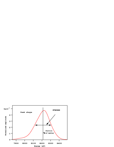
Figure 6: Standard asymmetric line shape obtained from the $\mu{}^{4}\mathrm{He}(2-1)$ transition. Cu contamination and continuous background have been subtracted. The peak surface is normalized to unity. The FWHM can be adjusted. The peak position is defined to be the position of the median, i.e., the center of gravity.

Figure 5 presents the spectrum for pure ${}^{4}\mathrm{He}$. The Lyman series between 8 and 11 keV and the Balmer series around 2 keV are clearly seen and the contaminant peaks are the same as in the muonic deuterium spectrum.

Figure 7: Average FWHM energy resolution of the CCDs in eV, obtained after fitting the $\mu\mathrm{He}(2-1)$ transition as well as the electronic lines with a peak shape given in Fig. 6. This curve was used to constrain the FWHM of the muonic deuterium and helium peaks.

Figure 8: X–ray energy spectrum of the $\mathrm{D}_{2}+{}^{4}\mathrm{He}$ mixture. The large peak represents the decay of the $(\mathrm{d}\mu{}^{4}\mathrm{He})^{*}$ molecule via an x ray of approximately 6.85 keV.

To further refine the fit, the muonic helium $\mu\mathrm{He}(2-1)$ transition was examined in detail to fully understand the true CCD response function for the line shape. This peak was chosen, even though it contained a small copper contamination (less than 1%), since it has high statistics and is well separated from the other peaks. The small copper contribution was subtracted. Since we could not use an analytical function for fitting the remaining asymmetric peaks, we interpolated the asymmetric peak shape of the $\mu\mathrm{He}(2-1)$ line, shown in Fig. 6, to fit the data correctly. As one can see, it looks like a Gaussian with an asymmetry on the left side. This same peak shape was then used to represent all other lines, replacing the Gaussian shape, and the spectra refit. In particular, the FWHM of each peak was obtained by using a scaling factor from the FWHM given in Fig. 6. In addition, all peak positions were defined by the center of gravity (not by the maximum). The values for the resolution of the $\mu\mathrm{He}(2-1)$ transition as well as the electronic lines are shown in Fig. 7. The fitting procedure was repeated for both the muonic deuterium and muonic helium spectra until a minimum $\chi^{2}$ was obtained. Replacing the Gaussian line shape with the final fit function including background parametrization and asymmetric line shapes reduced the $\chi^{2}_{dof}$ from 5 to about 1.4 for both spectra.

Figure 9: Resulting peak shape (dotted line) of the $(\mathrm{d}\mu{}^{4}\mathrm{He})^{*}$ molecular x–ray after fitting contaminants and background (solid line).

III.1.2 Spectra of the $\mathrm{D}_{2}+{}^{4}\mathrm{He}$ and $\mathrm{D}_{2}+{}^{3}\mathrm{He}$ mixtures

Figure 8 presents the energy spectrum of the $\mathrm{D}_{2}+{}^{4}\mathrm{He}$ mixture. In addition to the peaks from muonic deuterium, muonic helium, and the contaminants, a large x–ray peak from the decay of the $(\mathrm{d}\mu{}^{4}\mathrm{He})^{*}$ molecule appears around 6.8 keV. Again, the fitting procedure outlined above was used for all peaks except the molecular peak, for which theoretical curve has been calculated and is given in Ref. Belyaev et al. (1997). The difference in shape corresponding to decays of the $J=0$ and $J=1$ state, respectively, is negligible in our case. Hence, the calculated shape of Ref. Belyaev et al. (1997) was taken for the shape of this molecular peak. The positions of the maximum is a free parameter. We used two scaling factors to determine the amplitude and FWHM relative to the theoretical shape. Figure 9 shows the fit of the $\mathrm{D}_{2}+{}^{4}\mathrm{He}$ mixture in the region of the molecular peak (the fit was carried out over the whole energy region, 1.6 to 11.25 keV). The results are given in Table 2.

Figure 10: X–ray energy spectrum of the $\mathrm{D}_{2}+{}^{3}\mathrm{He}$ mixture. The wide peak represents the decay of the $(\mathrm{d}\mu^{3}\mathrm{He})^{*}$ molecule via an x ray of about 6.8 keV.

Table 2: Measured values of the two molecular $(\mathrm{d}\mu\mathrm{He})^{*}$ peaks. $\mathrm{E}_{\mathrm{d}\mu\mathrm{He}}$ is the energy of the peak maximum, $\Gamma_{\mathrm{m}}$ the measured FWHM, and $\Gamma_{\mathrm{d}\mu\mathrm{He}}$ the FWHM with the CCD resolution unfolded. $\mathrm{N}_{\mathrm{d}\mu\mathrm{He}}$ is the number of events in the peaks, corrected for the CCD efficiency.

Value	Unit	$(\mathrm{d}\mu^{3}\mathrm{He})$	$(\mathrm{d}\mu^{4}\mathrm{He})$
$\mathrm{E}_{\mathrm{d}\mu\mathrm{He}}$	[eV]	$6768\pm 12$	$6831\pm 8$
$\Gamma_{\mathrm{m}}$	[eV]	$914\pm 9$	$907\pm 8$
$\Gamma_{\mathrm{d}\mu\mathrm{He}}$	[eV]	$863\pm 10$	$856\pm 10$
$\mathrm{N}_{\mathrm{d}\mu\mathrm{He}}$		$(411\pm 23)\times 10^{3}$	$(196\pm 11)\times 10^{4}$

Figure 10 presents the spectrum of the $\mathrm{D}_{2}+{}^{3}\mathrm{He}$ mixture and Fig. 11 shows the same spectrum in the region of the molecular peak. The analysis of that spectrum was identical to the $\mathrm{D}_{2}+{}^{4}\mathrm{He}$ analysis with results also given in Table 2.

Figure 11: Resulting peak shape (dotted line) of the $(\mathrm{d}\mu^{3}\mathrm{He})^{*}$ molecular x–ray after fitting contaminants and background (solid line).

III.2 Relative intensities of the K series transitions in muonic ${}^{4}\mathrm{He}$

The relative intensities of the K series transitions in pure muonic ${}^{4}\mathrm{He}$ are given in Table 3. The errors include a statistical part (fit) and a systematic part (CCD detection efficiency). The main error comes from the CCD efficiency which is not surprising since the fit parameters for “CCD depletion depth” and “CCD window thickness” converge in a range of ($28\pm 2$) $\mu$m and ($35\pm 1$) $\mu$m respectively. The results are compared to Tresch et al. (1998) where no isotopic effect (${}^{3}\mathrm{He}$ or ${}^{4}\mathrm{He}$) was seen (last column of Table 3). The agreement is excellent for the K$\alpha$ transition, and the significant discrepancies of the other values are understood, since the measurement of Tresch Tresch et al. (1998) was carried out at a lower density, which explains the K$\beta$ decrease and the K$\gamma$ increase. In addition, our accumulated experience with CCD background and detection efficiency resulted in a better fit in this work but we realize that the errors given in Tresch et al. (1998) were underestimated with respect to the CCD efficiency correction.

Table 3: Relative intensities K_i/K_total (for $i=2,3,\ldots,\infty$) of the K series transitions for pure ${}^{4}\mathrm{He}$, corrected for CCD detection efficiency. The errors include both statistical and CCD efficiency errors. The last column shows the results from Tresch Tresch et al. (1998).

Transition	Ki/Ktotal	Ki/Ktotal
	[%]	[%] Tresch et al. (1998)
$\mu\mathrm{He}(2-1)$	$46.9\pm 4.5$	$47.0\pm 0.2$
$\mu\mathrm{He}(3-1)$	$27.9\pm 2.8$	$20.3\pm 0.1$
$\mu\mathrm{He}(4-1)$	$16.3\pm 1.7$	$19.8\pm 0.1$
$\mu\mathrm{He}(5-1)$	$6.2\pm 0.7$	$8.8\pm 0.1$
$\mu\mathrm{He}(6-1)$	$2.5\pm 0.4$
$\mu\mathrm{He}(7-1)$	$0.1\pm 0.3$
$\mu\mathrm{He}(\infty-1)$	$0.1\pm 0.1$	$4.1\pm 1.6$

III.3 Excited state transfer and the $\mathrm{q}_{1s}^{\mathrm{He}}$ probability

The $\mathrm{q}_{1s}$ value represents the probability for a newly formed light muonic atom to fully deexcite to the 1s state when the muon also has the possibility of transferring directly from an excited state to a heavier nucleus (cf. Fig. 1). In binary mixtures, the notation often includes the identity of the heavier nucleus, $\mathrm{q}_{1s}^{\mathrm{{}^{3}He}}$ for example.

Table 4: Number of events in the K series transitions of $\mu\mathrm{d}$ and $\mu{}\mathrm{He}$ in a gaseous mixture of deuterium and ${}^{4}\mathrm{He}$ as well as in a gaseous mixture of deuterium and ${}^{3}\mathrm{He}$. All values are corrected for CCD detection efficiency.

	$\mathrm{D}_{2}+{}^{4}\mathrm{He}$		$\mathrm{D}_{2}+{}^{3}\mathrm{He}$
Transition	$\mu\mathrm{d}$ [$\times 10^{3}$]	$\mu{}^{4}\mathrm{He}$ [$\times 10^{3}$]	$\mu\mathrm{d}$ [$\times 10^{3}$]	$\mu{}^{3}\mathrm{He}$ [$\times 10^{3}$]
$(2-1)$	$2915\pm 173$	$438\pm 26$	$1445\pm 86$	$805\pm 48$
$(3-1)$	$603\pm 21$	$154\pm 10$	$385\pm 14$	$287\pm 19$
$(4-1)$	$85.8\pm 3.4$	$38.6\pm 2.9$	$55.4\pm 2.8$	$61.9\pm 4.2$
$(5-1)$	$2.3\pm 2.8$	$15.9\pm 3.8$	$1.4\pm 2.3$	$15.4\pm 1.9$
$(\geq 6-1)$	$1.2\pm 1.8$	$10.9\pm 3.9$	$1.0\pm 1.5$	$4.0\pm 3.4$
total	$\mathrm{N}_{\mu\mathrm{d}}^{{}^{4}\mathrm{He}}(1s)=3608\pm 174$	$657\pm 29$	$\mathrm{N}_{\mu\mathrm{d}}^{{}^{3}\mathrm{He}}(1s)=1889\pm 87$	$1174\pm 52$

We begin our analysis with the $\mathrm{D}_{2}+{}^{4}\mathrm{He}$ mixture. The number of events in the K series transitions in $\mu\mathrm{d}$ and $\mu{}^{4}\mathrm{He}$ in the gaseous mixture of $\mathrm{D}_{2}+{}^{4}\mathrm{He}$ is given in Table 4. The sum of $\mu\mathrm{d}$ events represents the total number of $\mu\mathrm{d}$ which reach the ground state and is called $\mathrm{N}_{\mu\mathrm{d}}^{{}^{4}\mathrm{He}}(1s)$.

Part of the ${}^{4}\mathrm{He}$ events come from the direct capture of the muon by helium, the other part by excited state transfer from muonic deuterium. It was shown in Tresch et al. (1998) that in gaseous $\mathrm{H}_{2}+{}^{4}\mathrm{He}$ mixtures, excited–state transfer proceeds only to the levels $n=3$ and $n=2$ of $\mu^{4}\mathrm{He}$. A detailed comparison of Figs. 8 and 5 also shows that in the $\mathrm{D}_{2}+{}^{4}\mathrm{He}$ mixture there is a large enhancement of the K$\alpha$ and K$\beta$ He lines over the higher transitions. In addition, some L transitions can also be seen in Fig. 5. The fact that the L$\gamma$ transition (in Fig. 8) contains approximately $200\>000$ (efficiency corrected) events versus only 2000 for the L$\delta$ line further confirms the above hypothesis. Therefore the sum of the events from the $\mu\mathrm{He}(4-1)$, $\mu\mathrm{He}(5-1)$, and $\mu\mathrm{He}(\geq 6-1)$ transitions in $\mu{}^{4}\mathrm{He}$ is due to direct capture. Taking this sum from Table 4, one gets a measured number of direct capture, $\mathrm{N}_{\mathrm{dc}}^{\mathrm{m}}=(65.5\pm 6.2)\times 10^{3}$, where we added the errors quadratically.

In the spectrum from pure $\mu{}^{4}\mathrm{He}$ (see results in Table 3) the percentage sum of the K_i/K_total fractions for $i\geq 4$ is $25.20\pm 1.81$%. The $\mathrm{N}_{\mathrm{dc}}^{\mathrm{m}}$ therefore corresponds to 25.20% of the total number of K–series x rays in $\mu{}^{4}\mathrm{He}$ ($\mathrm{N}_{\mathrm{dc}}^{\mathrm{tot}}$). Thus, we deduced the total number of direct capture events $\mathrm{N}_{\mathrm{dc}}^{\mathrm{tot}}=(260\pm 43)\times 10^{3}$. This number will allow us to differentiate between direct capture and excited state transfer events in the K$\alpha$ and K$\beta$ intensities, measured in the mixture of deuterium and ${}^{4}\mathrm{He}$.

The numbers of K$\alpha$ and K$\beta$ events occurring with the direct capture, $\mathrm{N}_{\mathrm{dc}}^{\mathrm{K}_{\alpha}}$ and $\mathrm{N}_{\mathrm{dc}}^{\mathrm{K}_{\beta}}$, were obtained using the intensity ratios K_i/K_total determined in the pure $\mu{}^{4}\mathrm{He}$ spectrum and $\mathrm{N}_{\mathrm{dc}}^{\mathrm{tot}}$. The total number of $\mu{}^{4}\mathrm{He}$ K$\alpha$ and K$\beta$ events in the mixture is given in Table 4. The differences are due to excited state transfer from $\mu\mathrm{d}^{*}$. The number of K$\alpha$ and K$\beta$ events coming from excited state transfer, $\mathrm{N}_{\mathrm{exc}}^{\mathrm{K}_{\alpha}}$ and $\mathrm{N}_{\mathrm{exc}}^{\mathrm{K}_{\beta}}$, are the difference between the first two lines of Table 4 and the previously determined $\mathrm{N}_{\mathrm{dc}}^{\mathrm{K}_{\alpha}}$ and $\mathrm{N}_{\mathrm{dc}}^{\mathrm{K}_{\beta}}$. Therefore the sum of events from excited state transfer is $\mathrm{N}_{\mathrm{exc}}^{\mathrm{tot}}=(398\pm 47)\times 10^{3}$. Now $\mathrm{q}_{1s}^{{}^{4}\mathrm{He}}$ can be determined by

$$\mathrm{q}_{1s}^{{}^{4}\mathrm{He}}=\frac{\mathrm{N}_{\mu\mathrm{d}}^{{}^{4}\mathrm{He}}(1s)}{\mathrm{N}_{\mu\mathrm{d}}^{{}^{4}\mathrm{He}}(1s)+\mathrm{N}_{\mathrm{exc}}^{\mathrm{tot}}}=90.1\pm 1.5\,\%$$ (1)

where $\mathrm{N}_{\mu\mathrm{d}}^{{}^{4}\mathrm{He}}(1s)$ is the total number of $\mu\mathrm{d}$ Lyman x rays in the $\mathrm{D}_{2}+{}^{4}\mathrm{He}$ mixture (see Table 4).

The analysis carried out in the case of the $\mathrm{D}_{2}+{}^{3}\mathrm{He}$ mixture was the same as in the $\mathrm{D}_{2}+{}^{4}\mathrm{He}$ mixture with the additional hypothesis that the muonic cascade was the same in both $\mu{}^{3}\mathrm{He}$ and $\mu{}^{4}\mathrm{He}$. Pure $\mu{}^{3}\mathrm{He}$ was not measured (only $\mu{}^{4}\mathrm{He}$) for this work. However, Tresch Tresch et al. (1998) has shown no isotopic effects between the two gases.

Therefore, the $\mathrm{q}_{1s}^{{}^{3}\mathrm{He}}$ is determined as

$$\mathrm{q}_{1s}^{{}^{3}\mathrm{He}}=\frac{\mathrm{N}_{\mu\mathrm{d}}^{{}^{3}\mathrm{He}}(1s)}{\mathrm{N}_{\mu\mathrm{d}}^{{}^{3}\mathrm{He}}(1s)+\mathrm{N}_{\mathrm{exc}}^{\mathrm{tot}}}=68.9\pm 2.7\,\%$$ (2)

where $\mathrm{N}_{\mu\mathrm{d}}^{{}^{3}\mathrm{He}}(1s)$ is the total number of $\mu\mathrm{d}$ Lyman x rays in the $\mathrm{D}_{2}+{}^{3}\mathrm{He}$ mixture (Table 4).

III.4 Radiative branching ratio $\kappa_{\mathrm{d}\mu\mathrm{He}}$ of the $(\mathrm{d}\mu\mathrm{He})^{*}$ molecule

The radiative branching ratio $\kappa_{\mathrm{d}\mu\mathrm{He}}$ for the $(\mathrm{d}\mu\mathrm{He})^{*}$ molecular decay can be determined the same way as in Tresch et al. (1998) for the $(\mathrm{p}\mu\mathrm{He})^{*}$ molecule. $\kappa_{\mathrm{d}\mu\mathrm{He}}$ is given by

$$\kappa_{\mathrm{d}\mu\mathrm{He}}\cdot W=\frac{\mathrm{N}_{\mathrm{d}\mu\mathrm{He}}}{\mathrm{N}_{\mu\mathrm{d}}^{\mathrm{He}}(1s)}\,,$$ (3)

where $\mathrm{N}_{\mathrm{d}\mu\mathrm{He}}$ is the number of events in the molecular peak (see Table 2) and $\mathrm{N}_{\mu\mathrm{d}}^{\mathrm{He}}(1s)$ the total number of the $\mu\mathrm{d}$ Lyman series x rays in the mixture. $W$ is the probability of a $\mu\mathrm{d}_{\mathrm{1s}}$ forming a $(\mathrm{d}\mu\mathrm{He})^{*}$ molecule and is given by the equation:

$$W=\frac{\phi\mathrm{c}_{\mathrm{He}}\lambda_{\mathrm{d}\mu\mathrm{He}}}{\Lambda_{\mu\mathrm{d}_{1s}}}\,,$$ (4)

where $\phi$ is the atomic density of the mixture, normalized to LHD, $\mathrm{c}_{\mathrm{He}}$ is the helium atom proportion, $\lambda_{\mathrm{d}\mu\mathrm{He}}$ the ground state transfer rate from $\mu\mathrm{d}$ to He, and $\Lambda_{\mu\mathrm{d}_{1s}}$ the disappearance rate of muons from the $(\mu\mathrm{d})_{1s}$ level.

Table 5: Radiative branching ratio $\kappa_{\mathrm{d}\mu\mathrm{He}}$ of the $(\mathrm{d}\mu{}^{3}\mathrm{He})^{*}$ and $(\mathrm{d}\mu{}^{4}\mathrm{He})^{*}$ molecules. The errors are commented in the text.

	$\mathrm{d}\mu{}^{3}\mathrm{He}$	$\mathrm{d}\mu{}^{4}\mathrm{He}$
$\lambda_{\mathrm{d}\mu\mathrm{He}}\>(10^{8}\>\mbox{s}^{-1})$	$1.856\pm 0.077$	$\phantom{1}10.50\pm 0.21$
$\Lambda_{\mu\mathrm{d}_{1s}}\>(10^{6}\>\mbox{s}^{-1})$	$1.637\pm 0.032$	$3.159\pm 0.018$
$W$	$0.721\pm 0.073$	$0.856\pm 0.044$
$\kappa_{\mathrm{d}\mu\mathrm{He}}$	$0.301\pm 0.061$	$0.636\pm 0.097$

The so determined values for $\kappa_{\mathrm{d}\mu\mathrm{He}}$ and $W$ are given in Table 5 for both helium isotopes. The values for $\lambda_{\mathrm{d}\mu\mathrm{He}}$ and $\Lambda_{\mu\mathrm{d}_{1s}}$ (in Table 5) were taken from Gartner Gartner et al. (2000). While the errors for $\mathrm{N}_{\mathrm{d}\mu\mathrm{He}}$ and $\mathrm{N}_{\mu\mathrm{d}}^{\mathrm{He}}(1s)$ include both the statistical and systematic uncertainties, the errors in $\phi$ and $\mathrm{c}_{\mathrm{He}}$ given in Table 1 are purely systematic. The errors on $W$ and $\kappa_{\mathrm{d}\mu\mathrm{He}}$ were calculated by normal error propagation without specifying the type of error.

IV Discussions

IV.1 General features of the x–ray energy spectra

The spectra presented in Figs. 3, 4, 5, 8, and 10 deserve three general comments. First, the relative intensities of the muonic deuterium K$\alpha$ and K$\beta$ transitions are density dependent Lauss et al. (1998). Since the density changed between mixtures (see Table 1), the muonic deuterium K$\alpha$ peak is slightly enhanced over K$\beta$ in the $\mathrm{D}_{2}+{}^{4}\mathrm{He}$ mixture.

Second, the x–ray count rate for the $(\mathrm{d}\mu{}^{3}\mathrm{He})^{*}$ molecule is smaller than for the $(\mathrm{d}\mu{}^{4}\mathrm{He})^{*}$ molecule since in the $(\mathrm{d}\mu{}^{3}\mathrm{He})^{*}$ case the two–particle breakup channel is more prominent. Third, the relative helium/deuterium line intensities depend on the helium concentration (see Table 1).

IV.2 $(\mathrm{d}\mu{}^{3}\mathrm{He})^{*}$ and $(\mathrm{d}\mu{}^{4}\mathrm{He})^{*}$ molecules

Table 6: Theoretical and experimental energies of the maximum of the molecular peaks, in eV. For the experimental values, we also list the detector type. Our values are taken from Table 2.

Theory	$(\mathrm{d}\mu{}^{3}\mathrm{He})$		$(\mathrm{d}\mu{}^{4}\mathrm{He})$
	$J=0$	$J=1$	$J=0$	$J=1$
Belyaev Belyaev et al. (1997)	6766	6808	6836	6878
Czaplinski Czaplinski et al. (1997)	6760	6782	6836	6857
Experiment	$(\mathrm{d}\mu{}^{3}\mathrm{He})$		$(\mathrm{d}\mu{}^{4}\mathrm{He})$
Gartner Gartner et al. (2000)
Ge + Si(Li)	$(6.80\pm 0.03)\times 10^{3}$		$(6.88\pm 0.03)\times 10^{3}$
this work
CCD	$6768\pm 12$		$6831\pm 8$

In Table 6 our CCD results for the position of the maximum of the two molecular peaks are compared to theoretical predictions Belyaev et al. (1997); Czaplinski et al. (1997) and to results Gartner et al. (2000) obtained with Ge and Si(Li) detectors. The Ge and Si(Li) detector results seem to favor the J=1 state but the CCD results imply a preference for transitions from $J=0$. Even if the CCD results are more precise and the CCD statistics are significantly higher, it is difficult to decide for $J=0$ or $J=1$ since the results of both detector types are effectively compatible considering the errors. What can be said unambiguously is that the CCD results are in excellent agreement with both theoretical predictions for decay from the $J=0$ state. It should be stressed that both the Ge and Si(Li) and the CCD data were taken simultaneously during the experiment.

Table 7: Theoretical and experimental widths (FWHM) of the molecular peaks in eV. For the experimental values, we also list the detector type. Our values are taken from Table 2.

Theory	$(\mathrm{d}\mu{}^{3}\mathrm{He})$		$(\mathrm{d}\mu{}^{4}\mathrm{He})$
	$J=0$	$J=1$	$J=0$	$J=1$
Belyaev Belyaev et al. (1997)	$861\pm 3$	$858\pm 3$	$843\pm 3$	$848\pm 3$
Czaplinski Czaplinski et al. (1997)	$866\pm 3$	$867\pm 3$	$854\pm 3$	$855\pm 3$
Experiment	$(\mathrm{d}\mu{}^{3}\mathrm{He})$		$(\mathrm{d}\mu{}^{4}\mathrm{He})$
Gartner Gartner et al. (2000)
Ge + Si(Li)	$910\pm 30$		$910\pm 20$
this work
CCD	$863\pm 10$		$856\pm 10$

In Table 7 the CCD experimental FWHM widths for the molecular peaks are again compared with the theoretical predictions Belyaev et al. (1997); Czaplinski et al. (1997) and with the Ge and Si(Li) data Gartner et al. (2000). The CCD results are in very good agreement with theoretical predictions for both $J=0$ and $J=1$ states, but distinguishing between the two states is not possible due to the almost identical theoretical values. On the other hand, the results with the “classic” (Ge or Si(Li)) x–ray detectors are between 1.5 to 2.5 $\sigma$ away from theory. The somewhat smaller width of the ($\mathrm{d}\mu{}^{4}\mathrm{He}$) molecule predicted by theory is also hinted at by our CCD data.

IV.3 Radiative branching ratio $\kappa$

Table 8: Comparison of the theoretical and experimental radiative branching ratios $\kappa$ of the $(\mathrm{d}\mu\mathrm{He})^{*}$ molecules. Only Kravtsov Kravtsov et al. (1993) includes all three disintegration channels (the others neglect the Auger channel, given in Fig. 1).

		$\kappa_{\mathrm{d}\mu{}^{3}\mathrm{He}}$	$\kappa_{\mathrm{d}\mu{}^{4}\mathrm{He}}$	$\frac{\kappa_{\mathrm{d}\mu{}^{3}\mathrm{He}}}{\kappa_{\mathrm{d}\mu{}^{4}\mathrm{He}}}$
Kino Kino and Kamimura (1993)	$J=1$	0.234	0.503	0.465
Gershtein Gershtein and Gusev (1993)	$J=1$	0.18	0.41	0.44
Kravtsov Kravtsov et al. (1993)	$J=0$	0.31	0.45	0.69
	$J=1$	0.33	0.49	0.67
Belyaev Belyaev et al. (1995)	$J=1$	0.325	0.585	0.56
Belyaev Belyaev et al. (1996)	$J=0$	0.364	0.707	0.51
	$J=1$	0.309	0.568	0.54
this work		$0.301\pm 0.061$	$0.636\pm 0.097$	$0.47\pm 0.17$

Table 8 presents the different theoretical values for the radiative branching ratio. The calculations are those of Kino Kino and Kamimura (1993), Gershtein Gershtein and Gusev (1993), Kravtsov Kravtsov et al. (1993), and Belyaev Belyaev et al. (1995, 1996). Except for Kravtsov Kravtsov et al. (1993) who includes the Auger decay channel $\lambda_{e}$ (see Fig. 1), only $\lambda_{p}$ (break up) and $\lambda_{\gamma}$ (x ray) are calculated. The x ray channel relates to $\kappa_{\mathrm{d}\mu\mathrm{He}}$ via the ratio

$$\kappa_{\mathrm{d}\mu\mathrm{He}}=\frac{\lambda_{\gamma}}{\lambda_{p}+\lambda_{\gamma}+\lambda_{e}}\,.$$ (5)

The different theoretical $\kappa_{\mathrm{d}\mu\mathrm{He}}$ values are compared with our experiment in Table 8. The large isotopic effect predicted by theory is seen by our experiment which is in contradiction to the $(\mathrm{p}\mu\mathrm{He})$ case Tresch et al. (1998). In general the agreement between theory and experiment is good, however, the experimental errors are sizable.

IV.4 Ground state formation probabilities $\mathrm{q}_{1s}^{\mathrm{He}}$

Table 9: Comparison of the $\mathrm{q}_{1s}^{\mathrm{He}}$ probability in hydrogen–helium (Tresch Tresch et al. (1998)) and in deuterium–helium (this experiment) mixtures.

Mixture	$\mathrm{H}_{2}+{}^{3}\mathrm{He}$	$\mathrm{H}_{2}+{}^{4}\mathrm{He}$	$\mathrm{D}_{2}+{}^{3}\mathrm{He}$	$\mathrm{D}_{2}+{}^{4}\mathrm{He}$
$\mathrm{q}_{1s}^{\mathrm{He}}$ [%]	$50\pm 10$	$65\pm 10$	$68.9\pm 2.7$	$90.1\pm 1.5$

The meaning of $\mathrm{q}_{1s}^{\mathrm{He}}$ has been described in Section III.3. Our results for the deuterium–helium mixtures, Eqs. (1) and (2), are listed together with those for the hydrogen–helium mixtures Tresch et al. (1998) in Table 9. It is interesting to note that in both cases (hydrogen or deuterium) $\mathrm{q}_{1s}^{\mathrm{He}}$ is smaller for ${}^{3}\mathrm{He}$, and therefore, the excited state transfer is more probable for the lighter of the two helium isotopes. In the case of hydrogen–deuterium mixtures Lauss et al. (1996), $\mathrm{q}_{1s}^{\mathrm{He}}$ has been shown to depend on the concentration of the components of the mixture. The large difference seen in our case between $\mathrm{D}_{2}+{}^{3}\mathrm{He}$ and $\mathrm{D}_{2}+{}^{4}\mathrm{He}$ is therefore partially due to the differing helium concentrations (see Table 1). The second observation is that the $\mathrm{q}_{1s}^{\mathrm{He}}$ is significantly larger for deuterium, a result of consequence in the case of muon catalyzed fusion in deuterium–helium mixtures Knowles et al. (2001).

V Conclusions

The use of CCDs for low energy x–ray detection allowed for a complete energy measurement of muonic deuterium, helium, and molecular $(\mathrm{d}\mu\mathrm{He})$ x rays with excellent energy resolution and low background. The large CCD surface resulted in an increased solid angle and therefore in better statistics when compared to traditional Ge or Si(Li) detectors. Of course, results like transfer rates still need the usual x–ray detectors since the CCDs give no timing information. The simultaneous use of CCDs and other x–ray detectors allows for systematic error checks of the experiment since the CCD electronics is completely independent. In conclusion, the addition of CCDs permitted a characterization of all transfer parameters and some high precision results. Only the use of CCD detectors allowed the determination of the radiative branching ratio, a result which was long awaited by theorists.

References

• Breunlich et al. (1989) W. H. Breunlich, P. Kammel, J. S. Cohen, and M. Leon, Ann. Rev. Nucl. Part. Sci. 39, 311 (1989).
• Aristov et al. (1981) Y. A. Aristov et al., Yad. Fiz. 33, 1066 (1981), [Sov. J. Nucl. Phys. 33, 564–568 (1981)].
• Tresch et al. (1998) S. Tresch et al., Phys. Rev. A 58, 3528 (1998).
• Gartner et al. (2000) B. Gartner et al., Phys. Rev. A 62, 012501 (2000).
• Matsuzaki et al. (2002) T. Matsuzaki et al., Phys. Lett. B 527, 43 (2002).
• Kino and Kamimura (1993) Y. Kino and M. Kamimura, Hyp. Interact. 82, 195 (1993).
• Augsburger (2001) M. Augsburger, Ph.D. thesis, Université de Fribourg, Switzerland (2001), (unpublished).
• Egger (1999) J.-P. Egger, Hyp. Interact. 119, 291 (1999).
• Salem et al. (1974) S. I. Salem, S. L. Panossian, and R. A. Krause, At. Data and Nucl. Data Tables 14, 91 (1974).
• Belyaev et al. (1997) V. Belyaev, O. Kartavtsev, V. Kochkin, and E. A. Kolganova, Z. Phys. D 41, 239 (1997).
• Lauss et al. (1998) B. Lauss et al., Phys. Rev. Lett. 80, 3041 (1998).
• Czaplinski et al. (1997) W. Czaplinski, A. Kravtsov, A. Mikhailov, and N. Popov, Phys. Lett. A 233, 405 (1997).
• Kravtsov et al. (1993) A. V. Kravtsov, A. I. Mikhailov, and V. I. Savichev, Hyp. Interact. 82, 205 (1993).
• Gershtein and Gusev (1993) S. S. Gershtein and V. V. Gusev, Hyp. Interact. 82, 185 (1993).
• Belyaev et al. (1995) V. B. Belyaev, O. I. Kartavtsev, V. I. Kochkin, and E. A. Kolganova, Phys. Rev. A 52, 1765 (1995).
• Belyaev et al. (1996) V. B. Belyaev, O. I. Kartavtsev, V. I. Kochkin, and E. A. Kolganova, Hyp. Interact. 101/102, 359 (1996).
• Lauss et al. (1996) B. Lauss et al., Phys. Rev. Lett. 76, 4693 (1996).
• Knowles et al. (2001) P. E. Knowles et al., Hyp. Interact. 138, 289 (2001).