Analysing power $\boldsymbol{A_{y}}$ in the reaction $\boldsymbol{\vec{p}p\rightarrow\,pp\>\!\eta}$ close to threshold

Abstract

Measurements of the $\eta$ meson production with a polarised proton beam in the reaction $\vec{p}p\rightarrow\,pp\>\!\eta$ have been carried out at an excess energy of $Q=40\,$MeV. The dependence of the analysing power $A_{y}$ on the polar angle $\theta^{*}_{q}$ of the $\eta$ meson in the center of mass system (CMS) has been studied. The data indicate the possibility of an influence of p- and d-waves to the close to threshold $\eta$ production.

I Introduction

Several measurements on the $\eta$ meson production in the proton-proton interaction covering a 100 MeV excess energy range were performed at different accelerators. The determined total cross sections bergdolt:93 ; chiavassa:94 ; calen:96 ; calen:97 ; hibou:98 ; smyrski:00 , as well as their differential distributions calen:98 ; tatischeff:00 ; moskal:01-2 ; abdelbary:02 triggered intensive theoretical investigations aiming to understand the production mechanism on the hadronic and quark-gluon level.

In the theoretical descriptions of the $\eta$-production in nucleon-nucleon collisions the excitation of the $S_{11}(1535)$ resonance plays a decisive role. The hitherto performed studies with the aim to describe the total cross section show a dominance of this virtual $S_{11}$ nucleon isobar in the close-to-threshold production of the $\eta$ meson. The excitation of this intermediate state results from a one meson exchange (e.g. $\pi,\ \eta$ or $\rho$) between the two nucleons followed by a strong coupling of the $\eta N$ system to the $S_{11}$.

Near threshold the energy dependence of the total cross section results from a three-body phase space modified by a strong nucleon-nucleon final state interaction and a significant contribution of the attractive interaction in the $\eta p$ system. Since several existing models with different scenarios of the excitation describe the existing data well, a confrontation of the predicitions with other observables is needed in order to distinguish between them. The measurements with polarised beam should settle the on-going discussion whether the $\eta$ production is dominated by $\rho$ germond:90 ; laget:91 ; santra:98 ; gedalin:98 , $\omega$ vetter:91 or $\eta$ batinic:97 exchange. The interference between considered amplitudes causes a different behaviour – depending on the assumed scenario – e.g. of the $\eta$ meson angular distributions. These differences are too weak in the close-to-threshold region to discriminate between different models. Yet, the predictions of the analysing power depend crucially on the assumed mechanism faeldt:01 ; nakayama:02 .

So far the only measurement of the analysing power has been performed tatischeff:00 at an excess energy $Q=1805$ MeV. In the present experiment, the analysing power close to the production threshold is determined and results for the interference terms from contributing partial waves are presented. A comparison with theoretical predictions will be discussed in section V.

Section II contains the description of the experiment and the method to extract the $\vec{p}p\rightarrow\,pp\>\!\eta$ events. The following section introduces definitions and gives a theoretical overview. In section IV, the results are presented.

II Experiment

Measurements of the $\vec{p}p\rightarrow\,pp\>\!\eta$ reaction were performed at the internal experiment COSY-11 brauksiepe:96 at the COoler SYnchrotron COSY maier:97nim in Jülich with a beam momentum of p${}_{beam}=2.096\,$GeV/c corresponding to an excess energy of $Q=40\,$MeV. During the experiment, cycles of about ten minutes for the two different beam polarisations were adjusted.

Using a hydrogen cluster target dombrowski:97 in front of one of the regular COSY dipole magnets, the experimental facility acts like a magnetic spectrometer. Positively charged particles in the exit channel are bent towards the interior of the ring where they are detected in a set of two drift chambers. Tracing back the reconstructed trajectories through the magnetic field to the interaction point allows for momentum determination. Particle identification is achieved by a time of flight measurement over a distance of 9.4 m between two scintillation hodoscopes. For further details, the reader is referred to reference brauksiepe:96 . Figure 1(a) shows that the method allows for a clear separation between pions and protons and hence for the identification of events with two protons in the exit channel.

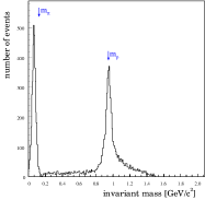
(a)

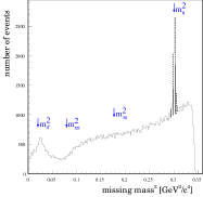
(b)

Figure 1: (a) Invariant mass spectrum for events with two reconstructed tracks. Besides the clear proton peak a second signal stemming from pions is observed. (b) Missing mass squared for events with two protons in the exit channel. Literature values groom:00 for particle masses are indicated by arrows.

The not registered particle system X – either a single meson (the $\eta$ in the present case) or a multi meson system – is identified by means of calculating its mass $m^{2}_{X}=(\mathbb{P}_{beam}+\mathbb{P}_{target}-\mathbb{P}_{1}-\mathbb{P}_{2})^{2},$ while $\mathbb{P}_{beam}$ and $\mathbb{P}_{target}$ denote the four momentum of the beam and target proton in the initial channel and $\mathbb{P}_{1},\ \mathbb{P}_{2}$ those of the two registered protons. The missing mass spectrum for events with two identified protons is shown in Figure 1(b) for the entire beam time. Besides the clear $\eta$-signal there is obviously a $\pi^{0}$-peak resulting from the reaction $\vec{p}p\rightarrow\,pp\>\!\pi^{0}$. Furthermore, a broad yield due to multi pion events with the lower limit given by $m_{X}^{2}=(2m_{\pi})^{2}$ and the upper limit by $m_{X}^{2}=(\sqrt{s}-2m_{p})^{2}=0.345\,$GeV²/c⁴ is observed. The increasing event rate towards higher missing masses is due to the higher acceptance of the COSY-11 detector for two protons with small momenta in the center of mass system (CMS).

The monitoring of the geometrical dimensions of the synchrotron beam and its position relative to the target moskal:01 enable to achieve a mass resolution of $\sigma_{m_{\eta}}=1.6\,$MeV/c². The much broader peak of the $\pi^{0}$ is due to the error propagation which worsens the mass resolution with increasing excess energy smyrski:00 .

III General Description

III.1 Definitions

A detailed theoretical derivation of the analysing power was recently published for the case of the $\vec{p}\vec{p}\rightarrow\,pp\pi^{0}$ reaction meyer:01 ; meyer:99 ; meyer:98 . For the $\eta$ production the description is analogue since in both measurements the initial channel is fixed to isospin I=1. Therefore, the different quantum numbers for $\pi^{0}$ (as a member of an isotriplet) and the isoscalar $\eta$ are irrelevant.

In the given experimental situation a convenient choice of the three axis is:

$$\hat{z}=\frac{\vec{p}_{beam}}{|\vec{p}_{beam}|},\quad\hat{y}=\frac{\vec{P}}{|\vec{P}|}\quad\mbox{and}\quad\hat{x}=\frac{\vec{y}\,\times\,\vec{z}}{|\vec{y}\,\times\,\vec{z}|},$$ (1)

where $\vec{P}$ indicates the polarisation of the COSY beam.

In the COSY-11 experiment, the two four momenta of the final protons $\mathbb{P}_{i}=(E_{i}^{*},\vec{p}_{i}^{\,*})$ are measured. The CMS momentum of the $\eta$ meson is $\vec{q}=-(\vec{p}_{1}^{\,*}+\vec{p}_{2}^{\,*})$. The proton momentum in the pp rest-system is denoted by $\vec{p}$ For later purposes, Figure 2 depicts the definition of the used polar- $(\theta)$ and azimuthal angle $(\varphi)$. The indices $p$ and $q$ will refer to the pp rest-system and the $\eta$ meson in the CMS, respectively. The angle $\theta_{p}$ will be choosen such, that $0\leq\theta_{p}\leq\pi/2$. This choice guarantees that all observables are invariant under the transformation $\vec{p}\rightarrow-\vec{p}$ as required by the identity of the two protons in the final state.

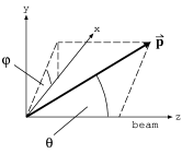
Figure 2: Definition of the angles. $\theta$ is defined as the angle between momentum vector and the z-axis, $\varphi$ between the x-axis and the projection of $\vec{p}$  onto the x-y-plane.

III.2 Observables

The differential cross section for a reaction with a polarised beam is given in terms of Cartesian polarisation observables by fick:71

$$\sigma(\xi)=\sigma_{0}(\xi)\left(1+\sum_{i=1}^{3}P_{i}\cdot A_{i}(\xi)\right),$$ (2)

where $P_{i}$ and $A_{i}$ denote the beam polarisation and the analysing power in the given reference frame, $\sigma_{0}(\xi)$ indicates the total cross section in case of no polarisation. In the upper formula, the abbreviation

$$\sigma(\xi)=\frac{d^{3}\sigma}{d\Omega_{p}d\Omega_{q}dE_{pp}}(\xi)$$

is used where $\xi$ denotes the set of the five variables which are kinematically completely describing the exit channel, namely $(\theta_{p},\ \varphi_{p},\ \theta^{*}_{q},\ \varphi^{*}_{q},\ E_{pp})$. The kinetic energy $E_{pp}$ of the two final protons in their CM system is given by $E_{pp}=\sqrt{s_{12}}-2m_{p}$ with $\sqrt{s_{12}}=2\sqrt{\vec{p}^{2}+m_{p}^{2}}$ as the energy in the pp subsystem.

In the given case of the general experimental conditions, the beam polarisation is – due to the magnetic fields in the accelerator – forced to be $\vec{P}=(0,P_{y},0)^{T}$ and hence formula (2) simplifies to

$$\sigma(\xi)=\sigma_{0}(\xi)\big{(}1+P_{y}\cdot A_{y}(\xi)\big{)}.$$ (3)

The asymmetry $\varepsilon$ – obtained from the difference in the yields with beam polarisation up and down – defined by

$$\varepsilon:=\frac{N_{\uparrow}-N_{\downarrow}}{N_{\uparrow}+N_{\downarrow}}$$ (4)

forms the basis for deducing the analysing power while $N_{\uparrow}\ (N_{\downarrow})$ denote the experimental number of events for spin up (down). With known luminosity $\mathcal{L}$, efficiency $\mathcal{E}$ and measured time $dt$, $dN$ is related to the cross section by $dN_{\uparrow,\downarrow}=\mathcal{E}\cdot\mathcal{L}\cdot\sigma_{\uparrow,\downarrow}\cdot dt$. In combination with equation (3), one can deduce from (4) that

$$A_{y}(\xi)=\frac{\mathcal{L}_{rel}\cdot N_{\uparrow}-N_{\downarrow}}{N_{\downarrow}\cdot P_{\uparrow}-\mathcal{L}_{rel}\cdot P_{\downarrow}\cdot N_{\uparrow}}(\xi),$$ (5)

where the relative time-integrated luminosity $\mathcal{L}_{rel}$ is defined by $\mathcal{L}_{rel}:=\frac{\int\mathcal{L}_{\downarrow}\cdot dt_{\downarrow}}{\int\mathcal{L}_{\uparrow}\cdot dt_{\uparrow}}$. In equation (5), the efficiency cancels out because of the independence on the spin as long as the bin size of $\Delta\xi$ is small enough so that the efficiency can be assumed to be constant.

With the definitions given in section III.1, the angular dependence of the spin-dependent cross section can be written as meyer:01 :

$$\sigma_{0}(\xi)A_{y}(\xi) = \Big{\{}\big{[}G_{1}^{y0}+G_{2}^{y0}(3\cos^{2}\theta_{p}-1)\big{]}\sin\theta^{*}_{q}+\Big{.}\big{[}H_{1}^{y0}+I^{y0}+H_{2}^{y0}(3\cos^{2}\theta_{p}-1)\big{]}\sin 2\theta^{*}_{q}\Big{\}}\cos\varphi^{*}_{q}$$ (6)

$$\ \>\!{}+\Big{.}\big{[}H_{3}^{y0}+K^{y0}+G_{3}^{y0}\cos\theta^{*}_{q}+H_{4}^{y0}(3\cos^{2}\theta^{*}_{q}-1)\big{]}\sin 2\theta_{p}\cos\varphi_{p}$$

$${}+\Big{.}(G_{4}^{y0}\sin\theta^{*}_{q}+H_{5}^{y0}\sin 2\theta^{*}_{q})\sin^{2}\theta_{p}\cos(2\varphi_{p}-\varphi^{*}_{q})+H_{6}^{y0}\sin 2\theta_{p}\sin^{2}\theta^{*}_{q}\cos(2\varphi^{*}_{q}-\varphi_{p})$$

The appearing literals denote interferences of partial wave amplitudes. The relative angular momentum of the two outgoing protons in their rest system is denoted by capital letters $l_{p}=S,P,D\ldots$, the one of the $\eta$ meson in the CMS by small letters $l_{q}=s,p,d\ldots$, while the usual spectroscopic notation is used. With this definition, the single terms $G_{k}^{y0},H_{k}^{y0},I^{y0}$ and $K^{y0}$ correspond to (PsPp), (Pp)², (SsSd) and (SsDs).

IV Results

In order to extract the assymetry from the measured spinup and spindown events one needs the relative luminosity and the average beam polarisation.

Via a simultaneous measurement of the proton-proton elastic scattering at the internal experiment EDDA albers:97 ; altmeier:00 the polarisation was determined for two time blocks:

time block 1 time block 2 P_↑ $0.381\pm 0.007$ $0.497\pm 0.006$ P_↓ $-0.498\pm 0.007$ $-0.572\pm 0.007$

The relative luminosity $\mathcal{L}_{rel}=\frac{N^{elas}_{\downarrow}}{\sigma^{elas}_{\downarrow}}\cdot\frac{\sigma^{elas}_{\uparrow}}{N^{elas}_{\uparrow}}$ was extracted via the elastic proton-proton scattering. To determine the elastic cross $\sigma^{elas}_{\uparrow,\downarrow}$ section according to equation (3) the analysing power was taken from altmeier:00 . With the number of events $N^{elas}_{\uparrow,\downarrow}$ resulting from the elastic pp-scattering $\mathcal{L}_{rel}$ was calculated according to the definition given above:

	time block1	time block 2
$\mathcal{L}_{rel}$	$1.004\pm 0.004{+0.002\atop-0.002}$	$0.949\pm 0.004{+0.001\atop-0.001}$

An integration of equation (6) over $\cos\theta_{p}$ and $\varphi_{p}$ leads to the disappearance of several terms provided the experimental angular distribution covers either the full phase space with a constant detector efficiency or symmetrical ranges. Figure 3 shows the angular distributions of $pp\eta$-events from a Monte-Carlo simulation which are neither symmetric around 90^∘ in case of $\varphi_{p}$ nor constant for both angles $\cos\theta_{p}$ and $\varphi_{p}$. Therefore, the evaluation of the analysing power requires an efficiency correction. To correct the data the efficiency $\mathcal{E}(\cos\theta_{p},\varphi_{p})$ is determined via Monte-Carlo simulations. Using a GEANT-3 code for each event a detection system response was calculated and the simulated data sample was analysed with the same programme which is used for the analysis of the experimental data. Weights $w(\cos\theta_{p},\varphi_{p})=1/\mathcal{E}(\cos\theta_{p},\varphi_{p})$ were applied during the final analysis of the experimental data and hence the corrected number of events reads:

$$N^{cor}=\frac{\sum\limits_{i}\sum\limits_{k}w_{i,k}N_{i,k}}{\sum\limits_{i}\sum\limits_{k}w_{i,k}}\,,$$ (7)

while $i$ and $k$ run over the bins $\varphi_{p}$ and $\cos\theta_{p}$, respectively. The error is deduced with $\Delta N_{i,k}=\sqrt{N_{i,k}}$ to be

$$\Delta N^{cor}=\frac{1}{\sum\limits_{i}\sum\limits_{k}w_{i,k}}\sqrt{\sum\limits_{i}\sum\limits_{k}w^{2}_{i,k}N_{i,k}}\,,$$

whereas the error of $w_{i,k}$ was neglected because of a much higher statistic for the Monte Carlo simulations, so that $\frac{\Delta w_{i,k}}{w_{i,k}}\ll\frac{\Delta N_{i,k}}{N_{i,k}}$. The influence of the strong proton-proton final state-interaction (FSI) was included via the description with a Jost-function goldberger:64 . Former acceptance studies on the dependence on the various Jost function prescriptions showed a change of the result of maximum 10% moskal:00 ; moskal:00-2 . An extensive discussion on the influence of the FSI reflecting itself in the density distribution of the Dalitz plot is given in moskal_wolke . Concerning that the FSI is known up to an accuracy of around 30% one can conclude that the upper limit for the total contribution to the error is approximately 3% which is negligible compared to the high overall error of this first data sample.

Figure 3: Angular distribution for the two proton angles $\cos\theta_{p}$ and $\varphi_{p}$ obtained via Monte-Carlo simulations.

Only after an efficiency correction one can remove the dependency from proton-coordinates in the analysis which is then the same as an integration over these variables so that equation (6) simplifies to:

$$\iint\frac{d^{2}\sigma}{d\Omega_{p}d\Omega_{q}}(\xi)\,A_{y}(\xi)\,d\cos\theta_{p}\,d\varphi_{p}=$$ (8)

$$2\pi\left(G_{1}^{y0}\sin\theta^{*}_{q}+(H_{1}^{y0}+I^{y0})\sin 2\theta^{*}_{q}\right)\cos\varphi^{*}_{q}.$$

Due to the restricting dipole gap $\varphi^{*}_{q}$ is dominantly peaked around 0^∘ – quite similar to the $\varphi_{p}$ distribution – but with a negligible peak around 180^∘ which is not shown here but verified with MC simulations. Therefore, the analysis was performed with one single $\varphi^{*}_{q}$-bin around $\pm 30^{\circ}$. Hence, equation (8) leads further to the separation of the (PpPs)-interference ($G_{1}^{y0}$) and the (Pp)²- and (SsSd)-terms ($H_{1}^{y0}$ and $I^{y0}$):

$$G_{1}^{y0} = \frac{1}{\pi^{2}}\int f(\cos\theta^{*}_{q})\,d\cos\theta^{*}_{q}\,,$$

$$H_{1}^{y0}+I^{y0} = \frac{2}{\pi^{2}}\int f(\cos\theta^{*}_{q})\cos\theta^{*}_{q}\,d\cos\theta^{*}_{q}\,,$$

with $f(\cos\theta^{*}_{q})=\int\limits_{-\frac{\pi}{6}}^{\frac{\pi}{6}}\int\limits_{0}^{2\pi}\int\limits_{0}^{1}\frac{d^{2}\sigma}{d\Omega_{p}d\Omega_{q}}(\xi)\,A_{y}(\xi)\,d\cos\theta_{p}d\varphi_{p}d\varphi^{*}_{q}$.

Defining $\bar{N}(\cos\theta^{*}_{q}):=\iiint N^{cor.}(\xi)\,d\Omega_{p}\,d\varphi^{*}_{q}$, it is straightforward to show analogue to equations (4) and (5) that the integrated analysing power defined by

$$\bar{A}_{y}(\cos\theta^{*}_{q}):=f(\cos\theta^{*}_{q})/\frac{d\sigma}{d\cos\theta^{*}_{q}}$$ (10)

can be determined via

$$\bar{A}_{y}(\cos\theta^{*}_{q})=\frac{\mathcal{L}_{rel}\cdot\bar{N}_{\eta,\uparrow}-\bar{N}_{\eta,\downarrow}}{P_{\uparrow}\cdot\bar{N}_{\eta,\downarrow}-\mathcal{L}_{rel}\cdot P_{\downarrow}\cdot\bar{N}_{\eta,\uparrow}}(\cos\theta^{*}_{q}).$$ (11)

The calculation of $\bar{A}_{y}$ needs the determination of the absolute $\vec{p}p\rightarrow\,pp\>\!\eta$ events $\bar{N}_{\eta,\uparrow\downarrow}$ in dependence of $\cos\theta^{*}_{q}$. In section II, the selection of the pp$\eta$ was discussed. The analysis was performed with 4 bins in $\cos\theta^{*}_{q}$ starting at $\cos\theta^{*}_{q}=-0.75$ with $\Delta\cos\theta^{*}_{q}=0.5$. A representative missing mass spectrum is shown in Figure 4(a) where the background is fitted by a polynomial function. From this spectrum the number of events $\bar{N}_{\eta+b}$ including background and $\eta$-event are extracted. Subsequently, this background is subtracted and the number of events $\bar{N}_{\eta}$ are determined (Figure 4(b)).

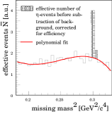
(a)

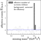
(b)

Figure 4: Spectra of the squared missing mass for events with two identified protons (a) with and (b) after subtraction of the background. The number of events was corrected according to equation (7).

For the two time blocks, an error weighted mean value for $\bar{A}_{y}$ is calculated. Figure 5 shows the analysing power as a function of $\cos\theta^{*}_{q}$. The extraction of $G_{1}^{y0}$ and $H_{1}^{y0}+I^{y0}$ with equations (LABEL:partialwellen) needs according to (10) the knowledge of $\frac{d\sigma}{d\cos\theta^{*}_{q}}$ which was taken from calen:98 . The fact that $\varphi_{q}\in[-\frac{\pi}{6},\frac{\pi}{6}]$ was considered with $\frac{d\sigma}{d\cos\theta^{*}_{q}}=\int^{-\frac{\pi}{6}}_{\frac{\pi}{6}}\frac{d\sigma}{d\Omega^{*}_{q}}\,d\varphi^{*}_{q}$ which is due to the isotropy of the cross section in $\varphi$

$$\frac{d\sigma}{d\cos\theta^{*}_{q}}\bigg{|}\raisebox{-8.5359pt}{$\scriptstyle-\frac{\pi}{6}\leq\varphi^{*}_{q}\leq\frac{\pi}{6}$}=\frac{\pi}{3}\frac{d\sigma}{d\Omega^{*}_{q}}.$$ (12)

Figure 5: Dependence of the analysing power on the center of mass polar angle $\theta^{*}_{q}$ of the $\eta$ meson.

The averaged values of $\bar{A}_{y}$ and the cross section used for the integrations in equations (LABEL:partialwellen) are presented in table 1.

$\boldsymbol{\rule[-9.0pt]{0.0pt}{22.0pt}\cos\theta_{q}}$	$\boldsymbol{\bar{A}_{y}}$	$\boldsymbol{\frac{d\sigma}{d\cos\theta_{q}}}$ [$\mu$b]
-0.75 $\pm$ 0.25	0.19 $\pm$ 0.21	0.31 $\pm$ 0.01
-0.25 $\pm$ 0.25	-0.02 $\pm$ 0.09	0.50 $\pm$ 0.01
0.25 $\pm$ 0.25	0.05 $\pm$ 0.06	0.50 $\pm$ 0.01
0.75 $\pm$ 0.25	-0.05 $\pm$ 0.06	0.31 $\pm$ 0.01

Table 1: Analysing power as a function of the emission angle $\theta_{q}$ of the $\eta$ meson in the CMS and the differential cross section obtained from calen:98 with equation (12).

Finally, the integrations of these values

$$G_{1}^{y0} = \frac{1}{\pi^{2}}\sum_{\cos\theta^{*}_{q}}\frac{d\sigma}{d\cos\theta^{*}_{q}}\bar{A}_{y}\cdot\Delta\cos\theta^{*}_{q}$$

$$H_{1}^{y0}+I^{y0} = \frac{2}{\pi^{2}}\sum_{\cos\theta^{*}_{q}}\frac{d\sigma}{d\cos\theta^{*}_{q}}\bar{A}_{y}\cos\theta^{*}_{q}\cdot\Delta\cos\theta^{*}_{q}\,.$$

result in

$$G_{1}^{y0}=(0.003\pm 0.004)\,\mu\mbox{b}$$

and

$$H_{1}^{y0}+I^{y0}=(-0.005\pm 0.005)\,\mu\mbox{b}\,.$$

V Comparison with theory

The present data on the $\eta$ meson production in nucleon-nucleon collisions referred to in section I show not only the 3-body phase space $Q^{2}$-dependency and a modification due to the nucleon-nucleon final state interaction but also a significant influence of the nucleon-meson interaction in the case of the $\eta p$ system. As mentioned above, several models describe the existing data quite well although they are based on different assumptions for the excitation mechanism of the $S_{11}$ resonance. For instance, Batinić et al. batinic:97 or Nakayama, Speth and Lee nakayama:02 found a dominance of $\pi$ and $\eta$-exchange in the analysis of $pp\rightarrow\,pp\>\!\eta$ while Fäldt and Wilkin faeldt:01 conclude a dominant $\rho$-exchange.

Polarisation observables may be the right tool to distinguish between the different models. Calculations for the analysing power in the reaction $\vec{p}p\rightarrow\,pp\>\!\eta$ show different results depending on the underlying assumption for the one meson exchange model. Figure 6 presents results taken from references faeldt:01 (dotted line) and nakayama:02 (solid and dashed lines) for $Q=10\,$MeV and 37 MeV. The authors of the latter reference conclude in the full model calculations a dominance of $\pi$ and $\eta$-exchange (solid line). The dashed curve represents a vector dominance model with an exclusion of $\pi$ and $\eta$-exchange for exciting the $S_{11}$ resonance. The triangles are the experimental results.

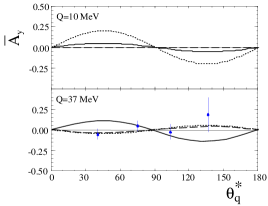
Figure 6: Analysing power for the reaction $\vec{p}p\rightarrow\,pp\>\!\eta$ in dependence on $\theta^{*}_{q}$ for the two excess energies $Q=10\,$MeV and 37 MeV.

The observable structure of the experimental values show a slight deviation from the $\sin\theta_{q}\cos\theta_{q}$-dependence of both models. It seems that the data favours the vector dominance exchange models. The more or less strong difference in the angular dependency of $A_{y}$ results from a vanishing $G_{1}^{y0}$ in both references. As this corresponds to the (PpPs)-term, an influence of the P-wave must be suspected but right now the experimental result for $G_{1}^{y0}$ is compatible with zero. A non-zero $G_{1}^{y0}$ would imply that $H_{1}^{y0}$ – describing the (Pp)² interference – should have a non negligible contribution, too. For further detailed studies the data are not yet precise enough to disentangle the sum of $H_{1}^{y0}$ and $I^{y0}$. At this time the results indicate the possibility of an influence of p- and d-waves to the close to threshold $\eta$ production.

VI Conclusion

The reaction $\vec{p}p\rightarrow\,pp\>\!\eta$ has been studied at an excess energy of $Q=40\,$MeV. The final state has been kinematically completely reconstructed and the analysing power has been determined. Qualitatively, the data seem to favour the calculations with dominant vector meson exchange but definitive conclusions cannot be drawn due to the large uncertainties of the data. To allow a more rigorous comparison with theoretical calculations higher statistics experiments are required and already scheduled for 2002 at COSY-11.

VII Acknowledgements

We are very grateful for the support of the EDDA-collaboration in determining the beam polarisation. Furthermore, we would like to thank C. Wilkin, C. Hanhart and K. Nakayama for very helpful discussions and contributions. Our special thanks go to Prof. Dr. J. Treusch, chairman of the board of directors of the research center Jülich, for undertaking a nightshift during the experiment.

This work has been supported by the International Büro and the Verbundforschung of the BMBF, the Polish State Committee for Scientific Research, the FFE grants from the Forschungszentrum Jülich, the Forschungszentrum Jülich directorates and the European Community - Access to Research Infrastructure action of the Improving Human Potential Programme.

References

- (1) A.M. Bergdolt et al., Phys. Rev. D 48 (1993) 2969.
- (2) E. Chiavassa et al., Phys. Lett. B 322 (1994) 270.
- (3) H. Calén et al., Phys. Lett. B 366 (1996) 39.
- (4) H. Calén et al., Phys. Rev. Lett. 79 (1997) 2642.
- (5) F. Hibou et al., Phys. Lett. B 438 (1998) 41.
- (6) J. Smyrski et al., Phys. Lett. B 474 (2000) 182.
- (7) H. Calén et al., Phys. Lett. B 458 (1999) 190.
- (8) B. Tatischeff et al., Phys. Rev. C 62 (2000) 054001.
-
(9)
P. Moskal et al., N Newsletter 16 (2002) 367.
e–Print Archive: nucl-ex/0110018 - (10) M. Abdel-Bary et al., (2002) e-Print Archive: nucl-ex/0205016
- (11) J. F. Germond and C. Wilkin, Nucl Phys. A 518 (1990) 308.
- (12) J. M. Laget, F. Wellers and J. F. Lecolley, Phys. Lett. B 257 (1991) 254.
- (13) A. B. Santra and B. K. Jain, Nucl Phys. A 634 (1998) 309.
- (14) E. Gedalin, A. Moalem and L. Razdolskaja, Nucl Phys. A 634 (1998) 368.
- (15) T. Vetter, A. Engel, T. Biro and U. Mosel, Phys. Lett. B 263 (1991) 153.
- (16) M. Batinić, A. Svarc and T. S. H. Lee, Phys. Scripta 56 (1997) 321.
- (17) G. Fäldt and C. Wilkin, Phys. Scripta 64 (2001) 427.
- (18) K. Nakayama, J. Speth, and T. S. H. Lee, Phys. Rev. C 65(2002) 045210.
- (19) S. Brauksiepe et al., Nucl. Instr. & Meth. A 376 (1996) 397.
- (20) R. Maier, Nucl. Instr. & Meth. A 390 (1997) 1.
- (21) H. Dombrowski et al., Nucl. Instr. & Meth. A 386 (1997) 228.
- (22) D. E. Groom et al., Eur. Phys. J. C 15 (2000) 1.
- (23) P. Moskal et al., Nucl. Instr. & Meth. A 466 (2001) 444.
- (24) H. O. Meyer et al., Phys. Rev. C 63 (2001) 064002.
- (25) H. O. Meyer et al., Phys. Rev. Lett. 83 (1999) 5439.
- (26) H. O. Meyer et al., Phys. Rev. Lett. 81 (1998) 3096.
- (27) D. Fick, Einführung in die Kernphysik mit polarisierten Teilchen (Bibliographisches Institut, Mannheim, 1997)
- (28) D. Albers et al., Phys. Rev. Lett. 78 (1997) 1652.
- (29) M. Altmeier et al., Phys. Rev. Lett. 85 (2000) 1819.
- (30) M. L. Goldberger and K. M. Watson Collision theory, Structure of matter series (John Wiley & Sons, Inc., New York, 1964)
- (31) P. Moskal et al., Phys. Lett. B 482 (2000) 356.
- (32) P. Moskal et al., Phys. Lett. B 474 (2000) 416.
-
(33)
P. Moskal, M. Wolke, A. Khoukaz, W. Oelert,
Prog. Part. Nucl. Phys. 49 (2002) 1.,
e-Print Archive: nucl-ex/0208004.