Abstract

The charge and magnetic form factors of light nuclei, mainly for mass number A$\leq$4, provide a sensitive test of our understanding of nuclei. A number of ”exact” calculations of the wave functions starting from the nucleon-nucleon interaction are available. The treatment of two-body effects needed in the calculation of the electromagnetic form factors has made significant progress. Many electron scattering experiments have provided an extensive data base from which the various (mainly elastic) form factors can be extracted. This review discusses the data and the determination of the form factors, and compares them to the results of theory.

PACS: 21.10.Ft, 21.45.+v, 25.30.Bf

1 Introduction

Few-body nuclei have long attracted particular attention in nuclear physics. This essentially is due to the fact that for these nuclei non-relativistic and sometimes relativistic calculations of the wave function with high accuracy starting from the nucleon-nucleon (N-N) interaction can be performed. For heavier nuclei models, or approaches with various approximations, have to be employed as a consequence of the complexity of many-body systems. In this case one largely looses the connection to the underlying, microscopic, physics.

For these light nuclei one then can best test our understanding of nuclei. Can they be described as essentially non-relativistic systems of nucleons interacting via the known N-N force, or do we have to go beyond this picture which has become known as the ”standard model of nuclear physics”? To which degree are nuclei relativistic systems? Do we need to explicitly allow for other constituents like excited nucleons, pions,..? Does the composite (quark) structure of the nucleon play an important role?

The few-body nuclei provide the possibility to study this rather wide spectrum of questions. While the deuteron is a very dilute system, the ${}^{4}He$ nucleus is the nucleus with largest density. In contrast to heavy nuclei, these nuclei have large gradients of the density which also can play an interesting role. The A=3 nuclei offer the possibility to study near-identical systems that differ only by the exchange of the role of protons and neutrons.

Significant progress has been made during the last decade in quantitatively computing the wave function of light nuclei. For many observables one today can be sure that differences in the calculated results reflect genuine differences in the physics included, and not simply approximations that needed to be made in the course of the calculation. A good part of these advances obviously is due to the vastly increased computational means that have become available.

Electron scattering provides an excellent tool for a detailed check of theoretical calculations of the wave functions of few-body nuclei, a test which often is more informative than what can be learned from integral observables such as energies of states or moments. Provided the experimental $(e,e)$ data go to large (four) momentum transfer $q$, the spatial structure of the one-body densities can (in Impulse Approximation IA) be studied with good spatial resolution, of the order of $1.5/q$.

As a consequence of the great interest in few-body form factors, many experiments on few-body nuclei have been performed over the last decades despite the experimental challenge they represent. We today have a rather complete set of data to which one can compare. An important aspect of the recent progress in $(e,e)$ experiments is the ability to measure polarization observables in the region of $q$ where they can help to discriminate between different theoretical predictions. Much of this progress has been made possible by the modern high-energy electron accelerators with high duty cycle such as MAMI or JLAB and the development of polarized sources, targets and polarimeters.

The form factors of light nuclei are of particular interest for another reason: Selected form factors, e.g. the isovector magnetic ones, exhibit a special sensitivity to exchange current contributions. For heavier nuclei the (magnetic) form factors show diffraction features at much lower momentum transfer already due to the structure of the wave function, and the contribution of two-body currents is much more difficult to isolate.

There is quite a vast literature on the few-body form factors — too vast for an exhaustive list of references without omitting significant work. These reviews have different areas of emphasis. The present review — written by an experimentalist — gives more than most others attention to data and ignores much of the detailed formalism of prime interest to more theory-oriented reviews. For general reviews on electron scattering see [1, 2, 3].

In this review, we first discuss the ingredients necessary for the calculation of the form factors. We then discuss for A=2,3,4,6,16 the data available, the determination of the optimal set of experimental form factors and their comparison to theoretical calculations. For the A=2 case, we include the transition form factor to the ¹S state.

2 Ingredients

2.1 Nucleon form factors

The charge- and magnetic form factors of nuclei are calculated from the wave function of the nucleons, obtained in most cases from a solution of the Schrödinger or Bethe-Salpeter equation for pointlike nucleons. In order to obtain the distribution of electric charge and magnetization as measured by $(e,e)$, the nucleon electromagnetic structure must be folded in. This can be achieved using the proton- and neutron electric and magnetic Sachs form factors $G_{e}$ and $G_{m}$ [4] known from elastic electron-nucleon scattering. In the one-body charge- and magnetic form factors, the (appropriate combination of) nucleon form factors come in as a multiplicative factor when going from the body form factor (calculated from the wave function) to the nuclear electromagnetic form factor. The tacit assumption is that the binding of the nucleon in the nucleus does not change its electromagnetic structure. One also assumes that the form factors for off-shell nucleons are the same as the ones for the free nucleon. For a reliable prediction of nuclear form factors we then need to know the nucleon form factors with adequate precision over the range of $q$ of interest for nuclear form factors.

The different nucleon form factors are known from $(e,e)$ experiments to a very different level of accuracy:

The proton magnetic form factor $G_{mp}(q)$ is well known from many experiments on electron-proton scattering. The data reach momentum transfers that go much beyond what is needed for a calculation of nuclear form factors (typically 8 $fm^{-1}$). Several parameterizations providing a very good fit to the data are available from Hoehler et al. and Mergell et al. [5, 6]; other parameterizations can be found in [7, 8], modern references are given in [6].

The proton electric form factor $G_{ep}(q)$ is well known at low and medium momentum transfers. At the higher momentum transfers, the data up to recently were somewhat contradictory. At high $q$, the magnetic contribution to the e-p cross section increasingly dominates, and a determination of $G_{ep}(q)$ via the usual Rosenbluth separation became more and more difficult with increasing $q$. Small systematic errors in the cross sections, which depend on a weighted sum of $G_{ep}^{2}(q)$ and $G_{mp}^{2}(q)$, started to play a big role.

The situation for $G_{ep}$ has recently improved with experiments that exploit polarization observables; when measuring the polarization of the recoil proton in scattering of polarized electrons from unpolarized hydrogen, the ratio $G_{ep}(q)/G_{mp}(q)$ becomes accessible [9, 10, 11]. This ratio is now well measured up to $q\sim 9fm^{-1}$. This covers the $q$-range of interest for nuclear form factors. The ratio $\mu_{p}G_{ep}/G_{mp}$ does deviate considerably from the naive expectation of 1 as given by the dipole formula. As it turns out, however, the new data on $G_{ep}(q)$ largely agree with the parameterization of Hoehler [5] which represents an often used standard for e-p scattering. This is shown

Figure 1: Ratio of $\mu_{p}G_{ep}/G_{mp}$ [9, 10, 11] together with the standard Hoehler parameterization (solid line, [5]) and the more recent fit of Mergell (dotted [6]).

in fig. 1 which displays the recent data together with the Hoehler parameterization. Certainly up to $q$ = 8 $fm^{-1}$, where reasonably accurate nuclear charge form factors are available, the proton charge form factor $G_{ep}$, even when used in terms of the venerable Hoehler parameterization, does not introduce a significant uncertainty.

The neutron magnetic form factor $G_{mn}(q)$, which is important when calculating nuclear magnetic form factors, also is a quantity that is rather difficult to determine experimentally. Due to the absence of a free neutron target, $G_{mn}$ has to be extracted from experiments on quasi-elastic electron scattering on the deuteron (or more complicated nuclei). In the case of inclusive $(e,e^{\prime})$ quasi-elastic scattering, the subtraction of the dominant proton contribution, and the corrections for deviations of the reaction mechanism from PWIA, lead to large systematic uncertainties. As a consequence, the data showed a large scatter [12].

Clean measurements, which do not depend unduly on the theory needed to interpret quasi-elastic scattering and to eliminate the dominating contribution from the proton, involve coincidence experiments of the type $d(e,e^{\prime}n)$ where scattering from the neutron in the deuteron can unambiguously be identified (save for corrections due to non-IA processes). Such experiments are today feasible with the modern high-duty cycle electron beam facilities, and we in the following will, as far as possible, only consider this type of data.

Several such experiments have been carried out recently [13, 14, 15] at NIKHEF and MAMI. The determination of the absolute efficiency of the detector used to identify the recoil neutron was measured at the proton-beam facility PSI which allowed one to produce intense high-energy tagged neutron beam of variable energy. At very low $q$, polarization observables can also be exploited as the theoretical understanding of the ${}^{3}He$ nucleus and the reaction mechanism has progressed to the point where polarized ${}^{3}He$ can serve as a polarized neutron target. In this case $G_{mn}$ can be obtained from the asymmetry of inclusive, single-arm quasielastic scattering [16, 17].

Figure 2: Data on the neutron magnetic form factor $G_{mn}$ divided by the dipole expression $G_{D}=(1+q^{2}/0.710(GeV/c)^{2})^{-2}$. The curve represents a fit with a continued-fraction parameterization [15].

The status of our experimental knowledge of $G_{mn}$ from coincidence measurements was clouded by two recent $(e,e^{\prime}n)$ experiments that claimed to provide accurate data [18, 19] which, however, greatly differed from the ones shown in fig. 2. Both experiments used $d(e,e^{\prime}n)$ to measure $G_{mn}$. Both relied, however, on a reaction with a three-body final state ($d(e,p)e^{\prime}n$ or $p(e,\pi)e^{\prime}n$) to produce the ”tagged neutron” which was needed to calibrate the neutron detector efficiency. Use of a three-body final state for tagging — without observation of the third particle, the scattered electron — is not possible as a matter of principle, and has been quantitatively shown to produce erroneous results [20, 21]. The respective results should be ignored.

Fig. 2 shows the status of today’s data on $G_{mn}$ [15]. Up to momentum transfers of $q\sim 5fm^{-1}$ the neutron magnetic form factor is known with excellent precision from coincidence experiments [13, 21, 15], and these results have been confirmed by experiments exploiting polarization observables [17, 16]. At the larger transfers one still has to rely on single-arm measurements [22]. At large $q$ the exploitation of $(e,e^{\prime})$ actually gets a bit easier than at low $q$ as the $G_{ep}$ contribution becomes small, so that the $(e,e^{\prime})$ cross section then depends mainly on $(G_{mp}^{2}+G_{mn}^{2})$, with comparable contributions from $G_{mp}$ and $G_{mn}$. On the whole, $G_{mn}$ is now known with adequate precision over the entire $q$-range needed for the calculation of nuclear magnetic form factors.

Jourdan et al. [15] have parameterized the modern data for $G_{mn}$ using a continued fraction expansion

$$G_{mn}=1/(1+q^{2}\cdot c_{1}/(1+q^{2}\cdot c_{2}/(1+...$$

with the constants $c_{1},...=3.260,-0.272,0.012,-2.5,2.5$ and $q$ in $GeV/c$. This fit also for the first time allows one to determine to better than 10% the magnetic radius of the neutron. It amounts to $0.873\pm 0.011fm$ (systematic errors included).

The neutron electric form factor $G_{en}$ is the quantity that is the poorest known among the nucleon structure functions. Only the slope $dG_{en}(q^{2})/d(q^{2})$ of $G_{en}$ at $q=0$ is well known from neutron-electron scattering [23]. The lack of knowledge on $G_{en}$ can occasionally really hamper the understanding of nuclear form factors. It does not always do it, as the smallness of $G_{en}$, which makes its experimental determination so difficult, at the same time leads often to a small contribution of the neutron to nuclear form factors. However, in interference response functions $G_{en}$ can play a much more important role.

The importance of $G_{en}$ for nuclear form factors can be appreciated by considering the charge form factor for an $N=Z$ nucleus. Nucleon finite size leads basically to a factor $(G_{en}(q)+G_{ep}(q))$ multiplying the body form factor calculated from the ground state wave function. At $q=4fm^{-1}$ the ratio $G_{en}$/ $G_{ep}$ amounts to 0.22 already [5], at larger $q$ it could be much larger if $G_{en}(q)$ continues to fall as slowly as present data for $q<4fm^{-1}$ seem to imply. Parameterizations such as the one of Gari and Krümpelmann [24] have predicted large ratios at large $q$, e.g. $G_{en}/G_{ep}$=1.4 at $q=9fm^{-1}$. Experiment [22] only provides an upper limit of $\sim 0.8$ (see fig. 3). The uncertainty in $G_{en}$  is of course particularly detrimental for ${}^{3}H$ [25] where the neutron charge form factor comes in with the double weight.

The determination of $G_{en}$ is difficult as there is no free neutron target; in addition, the measured electron-neutron cross section is largely dominated by the contribution from the magnetic form factor $G_{mn}$. In the past, $G_{en}$ therefore was mainly determined from electron-deuteron elastic charge scattering which eliminates the magnetic contribution. In this approach, the removal of the deuteron structure (deuteron body form factor), the subtraction of the proton contribution and non-IA contributions to the reaction mechanism lead to large systematic uncertainties, however. The most reliable determinations were probably those of Platchkov et al. [26] and Galster et al. [27] which, using various calculations of the deuteron wave function and non-IA contributions, provided values of $G_{en}$ up to 4 $fm^{-1}$. The resulting parameterizations have considerable systematic uncertainties due to both the deuteron input and the different theoretical results for the non-IA contributions [28, 29, 30, 31].

The neutron electric form factor can, in principle, also be determined via quasi-elastic electron-deuteron scattering, subtraction of the proton contribution and longitudinal/transverse (L/T) separation. The resulting uncertainties are substantial, however; at low $q$ the $G_{en}$ contribution is comparable to the experimental systematic uncertainties, at high $q$ (where it seems that the neutron and proton contributions are more similar in size) the overlap of quasi-elastic and Delta peaks makes difficulties. In fig. 3 we only show the results of Lung et al. [22] at very large $q$.

Figure 3: $G_{en}$ from double-polarization experiments of type $\vec{d}(\vec{e},e^{\prime}n)$, $\vec{{}^{3}He}(\vec{e},e^{\prime}n)$ or $d(\vec{e},e^{\prime}\vec{n})$ (for references see text). The parameterizations by Galster et al. and Platchkov et al. (for the deuteron $A(q)$ calculated with Paris and AV14 potentials, respectively) are given by dash-dotted and dashed lines. The extrapolation of the parameterizations to large $q$ are shown as dotted lines. The Hoehler $G_{ep}$ is also indicated as a dotted line. Also shown are some upper limits of $G_{en}$ from $d(e,e^{\prime})$ [22] at large $q$.

Today, $G_{en}$ can be determined via polarization observables in $(e,e^{\prime}n)$ experiments. The detection of the knocked out neutron — feasible at CW electron beam facilities — largely removes the contribution of the proton. The use of polarized electrons and polarized target (or, alternatively, measurement of the polarization of the recoil neutron) allows one to measure an interference term $G_{en}\cdot G_{mn}$ which, once $G_{mn}$ is known, provides a measurement of $G_{en}$.

Given the experimental difficulties of polarized targets or recoil polarimeters, only a few results from $\vec{d}(\vec{e},e^{\prime}n)$, $\vec{{}^{3}He}(\vec{e},e^{\prime}n)$ and $d(\vec{e},e^{\prime}\vec{n})$ are available [32]- [40] and the data still have fairly large uncertainties. Fortunately, however, these uncertainties are mainly statistical in nature, and thus can be improved upon with the progress in polarized target and polarimeter technology. The presently available set of $G_{en}$ data from double-polarization experiments is displayed in fig. 3. Clearly, the extent of the data still is far less than what is desirable as an input to the calculation of nuclear form factors of light nuclei.

2.2 N-N potentials

An important ingredient to the calculations of the few-body wave functions is the nucleon-nucleon (N-N) potential employed. As compared to other interactions occurring in physics, the N-N interaction has an unusually rich and complicated structure. It depends on the spin and isospin of the nucleons and their relative momentum. Only the long-range part, dominated by one-pion exchange, can easily be calculated. The construction of N-N potentials is a field that has a long tradition and covers many aspects which we here cannot possibly do justice to; so we refer the reader to the original literature (for a review see e.g. papers by Machleidt [41, 42]). Here, we only can mention a few aspects that are relevant for the specific few-body calculations discussed.

The various N-N potentials are all fit to the N-N (p-p and p-n) scattering data and the deuteron binding energy. Typically, the scattering data up to energies of $\sim$350$MeV$ are employed. At energies higher than 350$MeV$ inelasticities due to $\pi$-production etc. lead to a much more involved description of N-N scattering. While earlier potentials [43, 44, 45, 46] were generally fitted to the full set of data available, more recent fits [47, 48, 49] often have used a restricted data set [50] (see below).

Most often, the nuclear force is parameterized in terms of a sum of One Boson Exchanges (OBE). These OBE potentials for the longest range component mostly use the local version of the one-pion exchange potential. For the intermediate and short range the potentials are parameterized in different ways. The Argonne V18 potential developed by Wiringa et al. [47] has a one-pion exchange piece for the longest range, but uses essentially phenomenological parameterizations for the shorter ranges. The Nijmegen potential of Stoks et al. [48] uses empirical masses of existing mesons and meson distributions. All potentials are regularized at short distances by e.g. exponential cut-off factors. These cut-off form factors simulate the effect of the exchange of heavier mesons which have not been taken into account. Modern versions of these OBE potentials are ’charge dependent’, i.e. they provide different parameterizations for p-p, n-p and n-n.

The CD-Bonn OBE potential differs mainly in the use of a non-local one-pion exchange term, which is derived from a relativistic Lagrangian for meson-nucleon coupling. This leads to a non-local force with a tensor component which is substantially weaker off-shell. As a consequence, this potential predicts a deuteron D-state probability which is $\sim$0.8% smaller than the one predicted by other potentials (the other deuteron static properties are very similar). Also, the A=3 binding energy for the Bonn potential is 0.4–0.5$MeV$ larger.

Several potentials include more than OBE. The Paris [51] and full-Bonn [52] potentials include 2$\pi$-exchange (or phenomenological fits to it), and thus largely can do away with the fictitious $\sigma$-meson exchange. The two-pion contribution is calculated using time-ordered perturbation theory, or via a dispersion-relation analysis of $\pi-N$ scattering. Terms like the $\pi\rho$ and $\pi\omega$ exchange have been included as well [52]. The full-Bonn potential is more difficult to use in nuclear structure calculations due to its energy dependence, and can not consistently be used for cases of $>$2 nucleons; as an alternative, the energy-independent (but still nonlocal) Bonn-B potential has been derived by Machleidt et al. [41].

The modern OBE potentials fitted to the cleansed N-N scattering data base (see below), the V18, CD-Bonn and Nijm-II potentials, achieve a similarly good fit. The major difference between them shows up in the calculations of nuclear properties where off–shell properties of the force do matter. In particular, a force with a weaker off-shell tensor component leads to a stronger binding of the A$\geq$3 systems.

In the past, the potentials were usually fit to the full data base on N-N scattering. More recently, the Nijmegen group has performed a fit to the data employing different energy-dependent potentials for different partial waves. The $\chi^{2}$ of individual data points was then used as a criterion to keep the data, or remove them from the data set. A large fraction ($\sim$30%) was removed. The remaining, cleansed, data base can be fit with very good $\chi^{2}$, which makes it attractive to those groups constructing N-N potentials and therefore has been used to fit the modern potentials mentioned above.

This procedure of removing data is fine as long as the parameterized energy dependence used in the data elimination procedure is correct, and as long as enough degrees of freedom have been allowed for. That this is the case is by no means obvious. It can be checked by comparing the resulting phases to the ones obtained from single-energy phase shift analyses of the full data set. If there are significant differences (as judged by the error bar resulting from the single-energy analyses) then one must assume that the multi-energy analysis used to reject data was not general enough and introduced a bias. When looking at the comparison of

Figure 4: S-D mixing parameter $\epsilon_{1}$ resulting from single energy phase-shift analyses (data points, [53, 54, 55, 56]), the multi-energy fit used to cleanse the data set (dashed, [50]), the phases from the CD-Bonn potential (dotdash [49]) and the $V18$ potential (dotted, [47]) fit to this set.

phases resulting from single- and multi-energy analyses, one finds worrisome systematic differences in some phases. This is true in particular for the $\epsilon_{1}$ phase (see fig. 4) [47] which affects the strength of the tensor force and is responsible for the S-D transitions that play an important role for few-body systems (deuteron electrodisintegration, A=3 magnetic form factors).

When using OBE potentials in calculations of the wave function of light nuclei with A$>$2, one generally finds an underbinding, which amounts to 0.5–1 $MeV$ for A=3 and several $MeV$ for A=4. This indicates that it is also necessary to consider the role of the three-body force (3BF). Such a 3BF results in particular from the internal degrees of freedom of the nucleon which have been frozen out when describing nuclei in terms of interacting nucleons only.

The longest-range 3BF involves the intermediate excitation of the nucleon to the $\Delta$, and two pions exchanged with two other nucleons. This interaction, originally given by Fujita and Miyazawa [57], is attractive in light nuclei. When introducing the $\Delta$ degrees of freedom explicitly in the wave function, as done e.g. by P. Sauer and collaborators [58], one finds that the attractive contribution is significantly reduced by dispersive effects (energy dependence of effective N-N interaction). Other sources for a 3BF need to be considered as well.

Often used are variants of the Tucson-Melbourne force of Coon and collaborators [59, 60, 61] which are based on 2$\pi$ and $\pi\rho$ exchange. At short range these forces are phenomenologically adjusted to produce e.g. the correct binding energy of the A=3 systems and nuclear matter density. Alternatively, the Brazil 3BF is sometimes used [62].

A somewhat different approach is followed by the Argonne/Urbana group [63, 64] who also uses at long range a two-pion exchange shape, but at short range uses a purely phenomenological spin- and isospin-independent repulsive term, with parameters that are again adjusted to fit the binding energies of light nuclei.

For the time being, these three body forces all contain adjustable parameters. The calculation of the 3BF from first principles is still too difficult, as this force not only has to account for non-nucleonic degrees of freedom integrated out when describing nuclei in terms of nucleonic constituents; it to some degree has to account as well for relativistic aspects which are suppressed in the standard, non-relativistic, calculations.

2.3 Wave functions

In order to predict the various charge- and magnetic form factors as measured by electron scattering experiments, accurate wave functions of the nuclear ground states are the basic ingredient. These wave functions can be calculated employing a number of different techniques, some of which we will address in other chapters of this review. In this section, we only want to discuss in somewhat more detail the approaches that are used in the ”standard model of nuclear physics”. Often these approaches are non-relativistic, but for the deuteron relativistic calculations are available as well. The non-relativistic approaches calculate the nuclear wave function as a solution of the Schrödinger equation for nucleons interacting via one of the modern N-N potentials which reproduce the N-N scattering data with a good $\chi^{2}$. Calculations performed within this framework have reached a high state of perfection, and they have been applied to all of the light nuclei.

In this picture of the nucleus, one has already made significant simplifications. Rather than allowing for all sorts of constituents — nucleons, excited nucleons, mesons, … — one has projected onto a purely nucleonic basis.

For the deuteron the wave function depends only on the n – p relative distance (relative momentum). The solution of the Schrödinger equation for the corresponding one-body problem is fairly straightforward. Technical complications arise with the momentum-dependent N-N interactions such as the full Bonn N-N potential for calculations in coordinate space.

For the three-body system, a number of different approaches to compute the wave function within the above-mentioned frame work have been developed. Over the years, some of these approaches to calculate ground-state wave functions have been perfected to a high degree of reliability [65]-[68].

In the Faddeev approach the Schrödinger equation is reformulated in terms of three coupled equations separated according to the pair of nucleons that have interacted last. The sum of the three equations reproduces the Schrödinger equation. While the separation may appear to complicate the description, it actually corresponds to a simplification as, in the limit of three identical particles, the 3 equations differ only by a permutation of indices. The variables typically used (for the case of coordinate space calculations) are the relative distance vector x of two nucleons and the relative radius vector y of the third nucleon relative to the center of mass of the pair (Jacobi coordinates), or the corresponding momenta.

The spin- and isospin degrees of freedom of the three nucleons have to be treated explicitly such to satisfy the Pauli principle. Often the wave function components are decomposed according to the relative angular momentum of pairs of particles, or one particle relative to the CM of the other two. Truncations of the space in terms of the angular momenta allowed for often are necessary (and can be shown to be justified).

Accurate calculations today typically keep all channels where the interacting N-N pair is in partial waves with $j\leq 4$, which requires 34 channels. For scattering states at high nucleon momenta, more channels are included in accordance with the larger total angular momenta of interest. These Faddeev calculations can be done both in coordinate- or momentum space. The former has the advantage that the (for many observables not so important) Coulomb interaction can be included more easily.

In realistic calculations of the A=3 ground state wave function, one wants to include the effect of a three body force (3BF). This force is more short-ranged than the $\pi$-exchange force, and gives typically a 2% contribution to the potential energy.

For the momentum-space approaches, it has been shown by the group of Glöckle to be practical also to solve for the lower energies ($<$100$MeV$, say) the Schrödinger equation for continuum states [69], a great asset when one wants to access the rich physics information contained in the two- and three-body break-up channels.

The three-body Faddeev equations actually can be generalized to four nucleons. The corresponding Faddeev-Yakubovsky equations [70] still can be solved although the number of channels required for an accurate description of the observables grows very quickly with the number of nucleons.

During the last years, the Correlated Hyperspherical Harmonics (CHH) approach also has successfully been used to describe the A=3,4 bound states as well as the two-body continuum channels. The hyperspherical approach involves rewriting the Faddeev equations in terms of new coordinates which use (for the case of coordinate space representation) the hyperspherical radius which corresponds to the quadratic sum of the usual Faddeev radial variables x and y, and the angle between x and y. This hyperspherical approach has long been used, without too much success. Only with the introduction in the wave function of explicit N-N correlation operators, with parameters determined in a variational calculation, has this approach become a successful one. These correlation operators account for the strong state-dependent N-N correlations induced by the N-N interaction at small N-N distances. Explicitly allowing for these correlations, as done e.g. by Kievsky et al. [71], greatly accelerates the convergence of the calculation in terms of the number of hyperspherical harmonics that need to be included.

The most recent addition to the arsenal of methods are Variational Monte-Carlo (VMC) calculations. The VMC calculations [72, 63, 73] start with a trial wave function with a Jastrow core that includes single-particle orbitals LS-coupled to the desired J,M values. Pair and triplet spatial correlations are introduced from the very beginning. The Jastrow core is then acted on by products of two-body spin-, isospin- tensor- and spin-orbit correlation operators. Three-body correlation operators are included as well according to the 3BF used. The correlation operators allowed for thus contain the same operators as occur in the N-N interaction employed. The wave function is diagonalized in a basis of different Jastrow spatial symmetry components to project out the lowest state.

The VMC trial wave functions have typically 20-30 parameters. Using the Metropolis algorithm [74], the parameters are determined by minimizing the energy. Such calculations today are feasible up to A=10, and produce ground state energies that are already quite accurate ($\sim$ 1 $MeV$).

In the Greens Function Monte Carlo (GFMC) approach used by Carlson et al. and Pudliner et al. [75, 64], one starts with a trial wave function (often the VMC wave function) and operates on it with the imaginary time operator $e^{-(H^{\prime}-E_{0})\tau}$, where $H^{\prime}$ is a simplified Hamiltonian and $E_{0}$ is an estimate of the eigen value, with $\tau$ being the imaginary time. The excited-state components of the trial wave function will then be damped out for large $\tau$, leaving the exact lowest eigen state with the desired quantum numbers. The expectation value of $H$ is computed for the sequence of different ’times’ to verify the convergence. Differences between the simplified $H^{\prime}$ and the true $H$ are treated perturbatively.

These GFMC calculations converge to the essentially exact wave function. Difficulties due to the ”sign problem”, which limited the times $\tau$ one could go to, recently have largely been overcome (see e.g. [76]).

2.4 Two-body terms

The work on electromagnetic observables of few-body systems has shown that two-body terms of the nuclear electromagnetic operators give important contributions to the observables. The explanation of the longstanding discrepancy between theory and experiment of the $n+p$ radiative capture cross section [77, 78] and the deviation of the A=3 magnetic moments from theory [79] provided the first concrete evidence. These exchange terms influence both the electromagnetic current and charge operators. The theoretical treatment of these two-body terms has made great progress during the past 20 years, as documented in several review papers [80, 30].

The discussion below will start from the assumption that the nuclear system is basically non-relativistic, and that relativistic effects can be taken care of by the lowest-order expansion in $v/c$ (for calculations in a relativistic framework see sect. 3.5). Calculations of light-nucleus form factors in a fully relativistic frame work at present are still limited to the A=2 system; for the other nuclei we still have to rely on the non-relativistic approaches involving as complete as practical a set of relativistic corrections.

We begin by discussing the non-relativistic limit only. The electromagnetic current operator j in a nuclear many body system, which we address first, is related to the Hamiltonian $H$ of the system via the continuity equation ${\bf\bigtriangledown\cdot j}+i[H,\rho]=0$ where $\rho$ is the charge operator of the system. In non-relativistic nuclear physics one usually assumes that the Hamiltonian can be separated into a sum of single-nucleon kinetic energy terms $T$ and two-nucleon interactions $V$. As a consequence, the electromagnetic current operator j contains a sum of both single-nucleon and two-body operators. Two-body, or exchange, operators thus have to be present whenever the commutator between the N-N potential and the single-nucleon charge operator is non-zero. This is the case in particular for the isospin-dependent and velocity-dependent components of the N-N interaction. Such components occur prominently in the N-N interaction, as the long-range one-pion exchange interaction is isospin dependent, and thus leads to an important two-body operator. The non-locality of the N-N interaction also leads to a non-vanishing commutator, hence an exchange current operator needs to be taken into account [81].

Figure 5: Contributions to the two-body currents which are model-independent in the leading non-relativistic order. The exchange particles ’$\pi$’ and ’$\rho$’ are $\pi$- and $\rho$-like objects.

Further two- or many-body terms of the electromagnetic interaction would have to be considered once many-body forces between nucleons are allowed for. While such forces are indeed introduced to account for the binding energies of light nuclei (and nuclear matter) the corresponding many-body terms in the currents are still poorly understood.

The isospin dependent N-N interaction is associated with the exchange of charged particles. Within the simplest models, it involves the exchange of $\pi$’s and $\rho$’s. The corresponding interactions and the associated current operators which satisfy current conservation are known. This allows one to derive the two-body operators from the N-N interaction employed [82, 83, 84, 85]. The corresponding terms have been classified as ”model independent” by Riska [84]. In terms of a diagrammatic representation, these terms, accounting for the exchange of $\pi$’s and $\rho$’s, are displayed in fig. 5. By construction these terms respect gauge invariance. When dealing with realistic N-N interactions, these terms are replaced by exchange terms involving particles that are $\pi$-like (pseudoscalar exchange with quantum number $0^{-}$) and $\rho$-like (vector-meson type exchange with quantum numbers $1^{\pm}$), in accordance with the underlying structure of the N-N interaction [84, 86]. The identification of the $\pi$-like and $\rho$-like contributions is not necessarily dictated by the potential [85], so the qualification of ”model independent” has to be understood with the quotes. The additional two-body terms then are not necessarily constrained by current conservation.

These terms a priori do not account for the finite size of the nucleon. A simple (but not necessarily unique) approach to include the finite size replaces the coupling constants by vertex form factors. When using vertex form factors known from N-N scattering, additional vertex currents have to be introduced in order to respect current conservation. Fortunately, the numerical consequence of these form factors for few-body electromagnetic form factors is not great, as their effects in the $\pi$- and $\rho$-like terms largely cancel.

Other two-body terms related to other components of the N-N interaction, such a e.g. a velocity dependence, can be and have been included [87, 88], but are typically of lesser numerical importance.

While the above exchange current operators can be derived directly from the N-N interaction, and thus can be regarded as largely model independent, there are others that are not constrained by the continuity equation. These terms, addressed in the following, then are more uncertain.

Figure 6: Two-body contributions involving the Delta, and coupling to two different mesons.

These ”model dependent” terms (in the classification of Riska [84]) are associated with the excitation of virtual intermediate nucleon resonances and exchange operators involving more than one type of meson.

The most important model dependent transition-type exchange current operator involves excitation of an intermediary $\Delta_{33}$ resonance (see fig. 6), with the exchanged particle being $\pi$- or $\rho$-like. Processes involving higher nucleon resonances are suppressed by larger energy denominators. While some of the relevant coupling constants are known from experiment, others have to be derived via model calculations. For electron scattering at large $q$, the $q$-dependence of the couplings becomes a source of uncertainty. In calculations of the nuclear ground state wave function that allow for both nucleons and delta’s as done e.g. by Henning et al.  this term is, of course, included (in a non-perturbative way) in the wave function and does not appear as an exchange current contribution [89].

The second type of ”model dependent” two-body contribution accounts for terms of the type shown in fig. 6a. Such terms, which involve e.g. the $\rho\pi\gamma$ transverse isoscalar exchange current or the $\omega\pi\gamma$ current, are more uncertain due to the poorly known coupling constants involved. The $\rho\pi\gamma$ term can, depending on the observable, represent an important source of uncertainty at large $q$, the $\omega\pi\gamma$ and other terms are numerically not so significant. In most cases, though, the model-independent terms dominate, and these are well under control.

Coming to the two-body charge operators, the situation is less favourable. In the non-relativistic limit, there are no pion exchange contributions to the nuclear charge operator. The (longest range) pion exchange charge operator may be looked at as the contact term of the type shown in fig. 5b. This term, however, is already of relativistic order and cannot directly be linked to the N-N interaction employed to compute the nuclear wave function. The form of this two-body term (for the exchange of both $\pi$’s and heavier mesons) still is somewhat uncertain. To derive it one has to systematically reduce both the interaction and the electromagnetic current operator from a fully relativistic to a non-relativistic description. These contact-type contributions to the two-body charge operator are of considerable numerical importance when calculating the few-body C0 charge form factors.

When deriving the two-body charge operators by reduction from a relativistic description of the coupled system of meson and nucleon fields, such as e.g. done by Arenhövel et al. [31, 85], one also has to deal with the boost term which, at very high $q$, has a considerable effect.

The diagrams involving $\pi$- and $\rho$-exchange again need to be modified relative to the propagation of bare particles by vertex form factors in order to account for the finite size of the particles involved. These form factors can be taken as to be the same ones that occurred in the current operators, where they were constrained by current conservation and the N-N interaction employed.

As for the two-body currents, there are contributions to the two-body charge operator involving vector mesons, such as the $\rho\pi\gamma$ term (see fig. 6). These processes, as for the current operators, are of fairly short range and contribute only at very large momentum transfer.

The situation concerning exchange currents is different when considering the intrinsically relativistic approaches used by VanOrden et al. and Hummel and Tjon [90, 91] which solve the Bethe-Salpeter equation. If care is taken to insure that the truncations necessary in practical calculations do maintain current conservation, then (in PS-coupling) no two-body terms appear other than the pion-in-flight diagram (which usually gives a small contribution) and the ones due to the type of diagrams shown in fig. 6. The $\rho\pi\gamma$ diagram represents the dominant term, and introduces considerable uncertainty. Depending on whether a rather soft vertex form factor or a rather hard one (from e.g. Vector Dominance) is used, the deuteron $A(q)$ and $B(q)$ at large $q$ are close to the data, or too high.

3 Deuteron

3.1 Introduction

The deuteron, the only bound two-nucleon system, is one of the fundamental systems of nuclear physics. Accordingly, many studies, both experimental and theoretical, have been devoted to it. Of particular interest today is the degree to which the deuteron can be understood as a system of two nucleons interacting via the known nucleon-nucleon interaction.

When addressing, more specifically, the electromagnetic properties of the deuteron, the corresponding question concerns the ability to predict the three deuteron form factors starting from the calculated deuteron wave function and the nucleon form factors known from electron-nucleon scattering. At low momentum transfers predictions and data agree quite well when accounting for one-body terms only, at the higher momentum transfers, two-body contributions are known to be important. Whether quark degrees of freedom do need to be allowed for is still a matter of debate.

The approach traditionally taken for the two-nucleon system has been to derive the nucleon-nucleon (N-N) interaction from N-N scattering data, without inclusion of the information from the deuteron (other than the binding energy). The data for elastic electron-deuteron scattering then are used as a ”check” of our understanding of the N-N system.

The study of the electromagnetic form factors of the deuteron is complicated by the fact that the deuteron has spin one. As a consequence there are three form factors corresponding to the multipolarities $C0$, $M1$ and $C2$, needed to fully describe the electromagnetic structure. Without data on polarization observables — the measurement of which up to recently presented too many difficulties — only a combination of $C0$ and $C2$ could experimentally be determined, a fact that limited greatly our ability to fully exploit the information contained in the deuteron structure functions. This limitation fortunately now has largely been overcome.

The deuteron charge form factor is particularly interesting for the understanding of the role of exchange currents. To leading order, (non-relativistic) two body currents are absent due to their isovector character. The dominant two-body currents in the isoscalar charge form factor then are of relativistic, $v^{2}/c^{2}$, order. These currents still are less than perfectly understood. Therefore the $C0$ form factor is a good place to make comparisons between the non-relativistic approaches — supplemented by $v^{2}/c^{2}$ relativistic corrections — and the theories based on a fully relativistic approach.

The deuteron electromagnetic form factors most often are studied in order to check our understanding of the two-nucleon system. In parallel, however, the deuteron form factors are also exploited to get a better handle on the neutron form factors. In the past, much of our knowledge on the neutron charge form factor $G_{en}(q)$ came from precision studies of the deuteron structure function $A(q)$. Only very recently, experiments involving both polarized electrons and polarized target/recoil-nuclei have allowed us to get access to $G_{en}$ via other observables (see sect. 2.1). At large $q$, however, $G_{en}$ is still largely unknown, a fact that represents a serious handicap for the quantitative understanding of the deuteron charge form factors.

The deuteron is a very loosely bound system (probably the still best example for a ”halo nucleus”). Accordingly, many of the deuteron properties of relevance to strong-interaction physics concern the large-radius behaviour of the deuteron wave function which is well under control. With the electromagnetic form factors at the higher momentum transfers $q$, one does have the chance to access the shorter-range properties of the two-nucleon system. This makes the study of the deuteron form factors — especially the $C0$ form factor — particularly interesting.

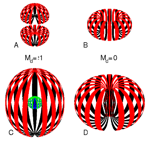
Figure 7: Equidensity surfaces of the deuteron for $m_{z}$ = 1,0 for high (A,B) and medium (C,D) values of the density [92]. Fig. A shows that for high density the deuteron is dumbbell like for m=$\pm$1, while B,C show a torus-like shape for m=0.

At small inter-nucleon distances, the deuteron actually has quite a bit more structure than appreciated when looking at the usual plots of the radial wave functions $u(r)$ and $w(r)$ of the $S$- and $D$-state, respectively. The strong tensor force at small $r$ leads to an interesting behaviour of the deuteron density: for spin-projection $m_{z}=\pm 1$ the equi-density contours have the shape of a dumbbell, for $m_{z}$=0 they have the shape of a donut, as displayed in fig. 7 from Forest et al. [92].

Traditionally, the calculations of the deuteron electromagnetic structure are compared to the structure functions $A(q)$ and $B(q)$ and, more recently, to the data on the polarization observable $T_{20}$ that are becoming available. In the present review, we mainly compare to the $C0$, $C2$ (and $M1$) form factors rather than $A(q)$ and $T_{20}$. This is done for two reasons. First, the individual $C0$ and $C2$ form factors are much more sensitive to the physics ingredients than $A(q)$. Second, the use of $C0$ and $C2$ allows us to more directly compare to the A=3 (T=0) and A=4 charge form factors.

We also want to deemphasize the discussion of the observable $T_{20}$ for another reason: this quantity refers to a specific scattering angle (although the dependence on the angle is weak as compared to the one on momentum transfer). It thus is better to avoid this dependence on angle altogether and concentrate on $C0$ and $C2$. Moreover, the physical significance of $T_{20}$ is rather convoluted (even if expressed in terms of the form factors $F_{00}$ and $F_{11}$, see ref. [92] and below). We therefore rather use the $C0$ and $C2$ form factors, which today can be determined with adequate precision from the experimental data.

3.2 Electron scattering data

Elastic electron-deuteron scattering has been investigated in many experiments, and the cross section data [93] - [116] today cover a large range of momentum transfers. Some of that data obviously is not very precise, other data, mainly of more recent origin, has reached accuracies down to the 1% level. In the analysis to be described below, we will employ the full set of world data today available. We discuss below in more detail only some of the sets.

The earliest measurements useable in todays determination of deuteron form factors, were performed at Stanford by Friedman et al. [107]. These measurements actually were aimed mainly at the neutron magnetic form factor, which was studied via magnetic scattering from the deuteron. The experiment of Rand et al. [113] provided the first more extensive set of data on the magnetic form factor measured at 180^∘. The main result of this experiment actually concerned threshold electro-disintegration, the process that later on [117] was recognized to be one of the showpieces for the contribution of meson exchange currents (see sect. 3.6).

The experiment of Elias et al. [106], performed at the Cambridge electron accelerator, provided data up to 6$fm^{-1}$. In this experiment, the electron beam was scattered from a target placed inside the synchrotron. Elastic scattering was identified by detecting the recoil deuterons using a quadrupole spectrometer. These data cover an important range in $q$, where few other data were available up to very recently. Some care is advisable in using this data: the deuteron spectra, measured with a combination of scintillators, spark chambers and range counters, appeared to show an unidentified constant ”background” of 20 $\div$ 50% under the deuteron peak. This ”background” was subtracted by the authors. After closer inspection of the deuteron spectra, and with the benefit of hindsight, it would appear that there actually was no significant background; rather, the deuteron peak (measured over too narrow a momentum region to allow one to identify a ”constant background”) was simply a bit wider than expected.

The Bonn synchrotron also contributed to the world supply of electron-deuteron data [104]. Using two magnetic spectrometers, the reaction products were detected in coincidence at both forward and backward angles, in order to perform a selfconsistent Rosenbluth separation. (Note that the last entries in table 2 of [104] seem to be inverted).

Data at the highest momentum transfers were measured by Arnold et al. at SLAC [96, 97, 101, 112] both at forward and backward angles. In both experiments scattered electron and recoil deuteron were detected in coincidence. For the case of the backward-angle scattering, the reaction products were detected at zero and 180^∘, respectively. This experiment identified for the first time the diffraction minimum occurring in $B(q)$ at $q\sim 7fm^{-1}$.

Two recent experiments at Jefferson Laboratory by Abbott et al. and Alexa et al. provided additional data [93, 94]. These experiments could reach very large momentum transfers due to the large beam intensities available at JLAB and the large acceptance of the spectrometers. While the hall-A experiment was carried out using the two high-resolution spectrometers, the hall-C experiment employed for the recoil-detection the magnetic channel built for the $T_{20}$ polarimeter (see below). In this latter experiment the spectrometer acceptance and target length were reduced on purpose in order to achieve a well known solid angle and spectrometer acceptance. At the time of the writing of this review, there still is a significant discrepancy between the two data sets; there is the suspicion that this is due to discrepancies in the determination of the beam energy.

Of particular interest to the precise determination of the deuteron form factors are the sets of data which have reached the highest accuracy. At the low and medium momentum transfers, these are the data of Galster et al., Berard et al., Simon et al.  and Platchkov et al. [27, 100, 114, 26]. Precision experiments on the deuteron face extra problems as compared to experiments involving heavier nuclei, for two reasons:
$\bullet$ Achieving a reasonably large target thickness involves in general the use of long liquid-deuterium targets. The determination of the acceptance of spectrometers for long targets requires a special effort. This poses particular problems for modern multi-element spectrometers which have a complicated acceptance function.
$\bullet$ Due to the low deuteron mass, the energy loss of the electron due to deuteron recoil is large. At the larger momentum transfers the deuteron elastic peak then overlaps with the quasi-elastic peak of the target windows. This in general requires to move the windows outside the spectrometer acceptance, or to detect electron and recoil deuteron in coincidence.

The experiment on e-d scattering carried out by Galster et al. [27] was performed at the DESY accelerator using the extracted beam. In this experiment the scattered electron and recoil deuteron were detected in coincidence in order to identify elastic scattering at the incident electron energy of 2.5 GeV. Galster et al. did a very precise comparison between e-p and e-d scattering, with the aim to determine from the deuteron cross section the small contribution of charge scattering from the neutron. This determination of $G_{en}$, performed up to momentum transfers of 4$fm^{-1}$, actually has withstood quite well the test of time.

The low-$q$ data of Berard et al. [100] were taken using cooled H₂ and D₂ gas targets, in the range of momentum transfer $q=0.2\div 0.7fm^{-1}$. The experiment essentially measured ratios of cross sections relative to Hydrogen; to get cross sections for the deuteron, normalization to absolute data on the proton is needed (for small corrections, see [118]).

The data of Simon et al. [114] covers the range 0.2 $\div~{}2fm^{-1}$. The experiment used both a low-temperature gas- and a liquid target, for both Hydrogen and Deuterium. The Hydrogen data taken with the gas target and a special small-angle spectrometer served as the absolute cross section standard, the data with the liquid targets were measured relative to that standard.

The experiment of Platchkov et al. [26] provided absolute data in the range $q=0.7\div 4.5fm^{-1}$ measured with a liquid Deuterium target. This experiment reached a very high accuracy, $\sim$1%. This became possible as the spectrometer acceptance was restricted to the purely geometric one, which is easily measured. The acceptance of the spectrometer for finite target length had been studied in detail using solid targets displaceable along the beam direction. The absolute efficiency of the detection system in the focal plane could be measured precisely by exploiting the redundancy of the various detector elements. Data taken with a liquid Hydrogen target were used to confirm the accuracy of the absolute cross section measurement. The Saclay group also provided data on magnetic scattering up to momentum transfers of $5.3fm^{-1}$ [98], measured at a scattering angle of 155^∘.

Some of the deuteron data [93]–[116] listed above have been taken by determining the overall normalization using electron-proton scattering. The cross sections given in the publications were obtained by normalizing the measured ratios using the best information on the parameterization of the proton form factors available at the time. Today, we have a set of more accurate and more complete proton data, and a comprehensive fit to all the data. It is therefore advisable to renormalize the corresponding deuteron data using the fit to todays world data on the proton [6] in order to obtain the most accurate absolute deuteron data.

For a detailed investigation of the form factors and their uncertainties, it is very important to account for the systematic errors of the data. Their effect in general is much larger than the uncertainty due to the statistical errors. In the publications cited, the systematic uncertainties often are not adequately discussed, and several times important sources of systematic errors other than normalization (e.g. electron beam energy, beam halos) are not even mentioned. For the data sets that have a particular weight in the determination of the form factors, one can consult the corresponding thesis works [119]– [124] in order to extract a reasonable estimate for the relevant systematic uncertainties.

During the last years, it has increasingly become possible to measure not only cross sections, but also spin observables. The knowledge of these spin observables is imperative if one wants to separate the two contributions of the $C0$ and $C2$ multipolarities to the $A(q)$ structure function. The separation of $C0$ and $C2$ is of particular interest in the region of the predicted diffraction zero of the $C0$ form factor, near $q=4fm^{-1}$. To separate $C0$ and $C2$ one needs data involving tensor spin observables.

Two techniques basically are available to measure such spin observables:

• At storage rings, one can use polarized, internal deuteron gas targets from an atomic beam source. The high intensity of the circulating electron beam allows one to achieve acceptable luminosities despite the very low thickness of the gas target.

• At facilities with external beams, one can use polarimeters to measure the polarization of the recoil deuterons. High beam intensities are a prerequisite as the polarization measurement, which requires a second reaction of the deuteron, involves a loss of a few orders of magnitude in count rate.

A further potential approach, the use of an external polarized target (such as $ND_{3}$ at very low temperature [125]) has not yet been employed, as the luminosities reachable with these targets were not sufficient. This in part is also related to the difficulties of making, instead of the usual vector-polarized targets, a tensor-polarized target as needed for the separation of $C0$ and $C2$.

The pioneering experiment on e-d scattering involving polarization observables was performed by Schulze et al. [126] at Bates. The polarimeter employed made use of the ${}^{3}He(\vec{d},p)^{4}He$ reaction, which represents an efficient analyzer of the tensor polarization for deuterons with very low momentum. This experiment provided data near $q\sim 2fm^{-1}$.

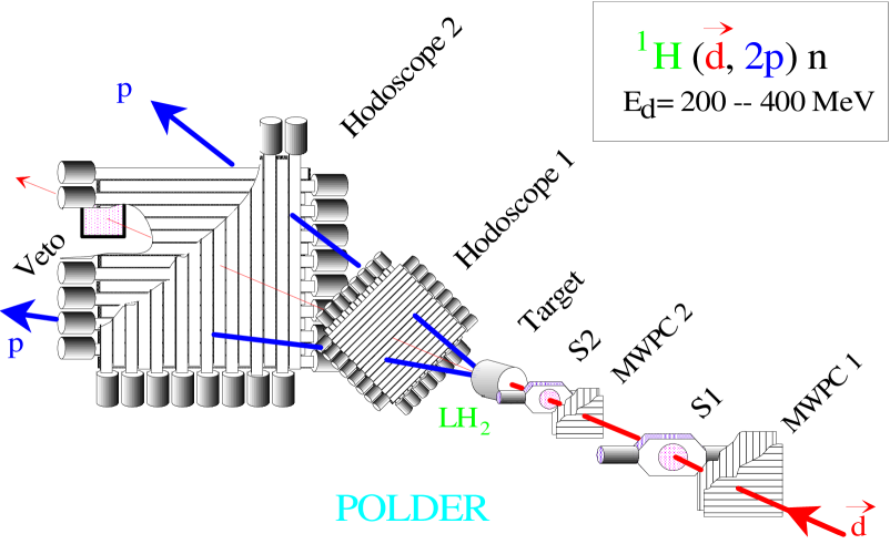
Figure 8: POLDER deuteron polarimeter used in the experiment of Abbott et al. [93]. The deuteron track is measured before the $\vec{d}+p\rightarrow p+p+n$ reaction using multi-wire proportional chambers. The two protons are detected using the hodoscope counters.

The first experiment with an internal electron beam and a gas-jet polarized target was performed at the VEPP-storage ring in Novosibirsk [127]. The data cover the region near 1$fm^{-1}$ momentum transfer. The follow-up experiment at VEPP [128] reached 3$fm^{-1}$, but had rather large statistical uncertainties.

These early experiments did not yet cover the region where the separation of $C0$ and $C2$ is expected to provide new information, but they showed that — with a suitable increase in luminosity and polarimeter efficiency — the determination of polarization observables would be practicable.

Higher momentum transfers could be reached using external beams and different types of polarimeters. The experiment of The et al.  [129], performed at the Bates accelerator, used a polarimeter based on $\vec{d}-p$ elastic scattering. With this setup it became possible to reach the region of the zero crossing of the $C0$ form factor at 4.4$fm^{-1}$.

Further measurements using an internal tensor-polarized gas target were carried out at the AMPS storage ring [130, 131]. The deuterons were produced using an atomic-beam source which injected the deuterons into a storage cell traversed by the electron beam. Scattered electron and recoil deuteron were measured in coincidence. This experiment provided $T_{20}$-values up to a momentum transfer of 3.2$fm^{-1}$.

The highest momentum transfers were reached in the recent experiment performed at JLAB by Abbott et al. [93]. With this experiment the data could be extended beyond the diffraction maximum of the $C0$ form factor, reaching 6.7$fm^{-1}$. This became possible with the construction of a polarimeter optimized for the high deuteron momenta, a polarimeter based on the $\vec{d}+p\rightarrow p+p+n$ break-up reaction depicted in fig. 8. This experiment also resolved a worrying discrepancy between the data and theory in the 4–5$fm^{-1}$ region where the normally most successful calculations seemed to lie significantly above the previous data.

Figure 9: World data for the tensor analyzing power $T_{20}$ for electron-deuteron scattering as function of momentum transfer (the slight dependence on scattering angle has not been removed).

In fig. 9 we display the $T_{20}$ data which today are available. Additional data have been measured for $T_{21}$ and $T_{22}$. These quantities, however, are not very constraining in separating the multipolarities $C0$ and $C2$; rather, they serve as consistency checks.

3.3 Experimental form factors

Here we use the world data on electron-deuteron scattering up to high momentum transfer to determine the various form factors. Some 340 data points on e-d scattering are available for momentum transfers below 8$fm^{-1}$ (the higher transfers are ignored for the moment as the experimental information is more fragmentary).

As discussed in more detail in section 3.4, the experimental cross sections are first converted to effective PWIA cross sections by removing the Coulomb distortion effects. This is done by multiplying the experimental cross section $\sigma(E,\theta)$ with the calculated ratio $\sigma_{1.Born}(E,\theta)/\sigma_{2.Born}(E,\theta)$. These $\sigma^{PWIA}$ then can be interpreted in terms of PWIA.

The deuteron cross sections measured in the various experiments [95]-[116] contain contributions from the form factors of multipolarity $C0$ (charge monopole), $M1$ (magnetic dipole) and $C2$ (charge quadrupole), which in turn determine the two structure functions $A(q)$ and $B(q)$:

$$\sigma(E,\theta)^{PWIA}=\sigma_{Mott}(E,\theta)[A(q)+B(q)~{}tg^{2}(\theta/2)]$$

where $\sigma_{Mott}$ includes the recoil factor, with

$$A(q)=F_{C0}^{2}(q)+(M_{d}^{2}Q)^{2}\frac{8}{9}\tau^{2}F_{C2}^{2}(q)+(\frac{M_{d}}{M_{p}}\mu)^{2}\frac{2}{3}\tau(1+\tau)F_{M1}^{2}(q)$$

$$B(q)=(\frac{M_{d}}{M_{p}}\mu)^{2}\frac{4}{3}\tau(1+\tau)F_{M1}^{2}(q)\hskip 14.22636ptwith\hskip 14.22636pt\tau=q^{2}/(4M_{d}^{2})$$

In the above equations, $M$ are the masses, $\mu$ the deuteron magnetic moment in units of magnetons, $Q$ the quadrupole moment and $q$ is the four momentum transfer (¿0). All the $F$-form factors are normalized to $F(0)=1$.

Up to recently the study of the form factors in general was limited to the $A(q)$ and $B(q)$ structure functions. With the polarization data that became available during the last years [126, 127, 128, 116, 130], one also can perform an analysis of the world data in terms of the form factors $F_{C0}(q)$, $F_{M1}(q)$, $F_{C2}(q)$. The tensor polarization observables give a handle to separate the contributions of $C0$ and $C2$. In particular

$$T_{20}=-(\frac{8}{3}\tau F_{C0}F_{C2}QM_{d}^{2}+\frac{8}{9}\tau^{2}F_{C2}^{2}Q^{2}M_{d}^{4}+\tau(\frac{1}{3}+\frac{2}{3}(1+\tau)~{}tg^{2}\frac{\theta}{2})F_{M1}^{2}(\frac{M_{d}}{M_{p}}\mu)^{2})/\sqrt{2}(A+Btg^{2}\frac{\theta}{2})$$

contains the interesting interference term $C0\cdot C2$. The other tensor observables, $T_{21}$ and $T_{22}$, are not so useful.

The separation of $A(q)$ and $B(q)$ (or $F_{C0}(q)$, $F_{M1}(q)$, $F_{C2}(q)$) in the past often has been done by the experimental groups providing the cross section data. In most cases, the individual experiments measured cross sections that were dominated by either $A(q)$ or $B(q)$, so that the ”Rosenbluth separation” could simply be done by subtracting the non-dominating structure function using the best values known at the time.

Here, we rather concentrate on a more reliable approach which involves a fit of the unseparated world cross sections with a parameterization of $A(q)$ and $B(q)$ simultaneously. This allows one to use the full set of data today available to determine all form factors. The ”Rosenbluth separation” thus is done implicitly during the fit of the data. As the parameterizations of $A(q)$ and $B(q)$ provide continuous functions, this approach also takes care of the problem that rarely the forward-angle and backward-angle data are available at exactly the same $q$. For the standard Rosenbluth separation this usually implies somewhat obscure interpolations or extrapolations. The same reasoning applies when determining the three form factors $C0$, $M1$ and $C2$ by adding the polarization observables.

In order to analyze the deuteron data, the various form factors are parameterized using a flexible functional form. From these form factors, one calculates cross sections in PWIA, and fits the parameters to the data (already corrected for Coulomb distortion).

We here discuss the results obtained with the Sum-of-Gaussians (SOG) parameterizations [132] for the $F$’s or, alternatively, $A(q)$ and $B(q)$. The form factors are written as

$$F(q)=e^{-\frac{1}{4}q^{2}\gamma^{2}}\sum_{i=1}^{n}\frac{Q_{i}}{1+2R_{i}^{2}/\gamma^{2}}\left(cos(qR_{i})+\frac{2R_{i}^{2}}{\gamma^{2}}\frac{sin(qR_{i})}{qR_{i}}\right)$$

For the comparison to theory mainly the $q$-space version is of interest a priori. In coordinate space, this parameterization for $F_{C0}(q)$ corresponds to the Fourier transform of a density $\rho(r)$ written as a sum of (symmetrized) gaussians that are placed at arbitrary radii $R_{i}$, with amplitudes $Q_{i}$ that are fitted to the data, and a fixed width $\gamma$.

The choice of this parameterization is governed by the following considerations. To extract form factors not biased by the choice of the analytical form, one needs a parameterization that in principle is totally general, with restrictions that can be justified on physical grounds. In the limit $\gamma\rightarrow 0,R_{n}\rightarrow\infty$ (hence $n\rightarrow\infty$) the SOG is a perfectly general basis. For a fit of the data, one introduces two restrictions: 1) The gaussians are given a finite width $\gamma$. In both $\rho_{ch}(r)$ and $\rho_{m}(r)$ we do not expect any structure that is significantly smaller than allowed for by the proton size. Accordingly, $\gamma$ is defined via the $rms$-radius $\gamma$ $\sqrt{3/2}=0.6fm$. It has also been verified that with this value the form factors from several theoretical calculations can be accurately represented up to the largest $q$. This finite width essentially imposes that the form factors on average fall no slower than the proton form factor. 2) The gaussians are placed at radii $R_{i}\leq R_{max}=10fm$. This is justified given the fact that, from independent knowledge on the behavior of wave functions at large radii, one can easily specify the radius at which the tails of densities give no significant $(<10^{-3})$ contribution to $F(q)$. A finite $R_{max}$ imposes that the form factor cannot oscillate in $q$-space more quickly than with a minimal wave length $\Delta q\propto 1/R_{max}$.

The data have been fitted with the SOG parameterization, and 10 free parameters (for $r<4fm$) for each structure function (for the treatment of the region $4<r<10$ fm see sect. 3.4). The data set for the deuteron is thus fitted with a total of 30 free parameters (20 for the fit of $A(q)$, $B(q)$).

The statistical error of the fit is easily calculated using the error matrix. The systematic errors, which in general are the dominating ones, have been evaluated by changing each individual data set by the quoted error, and refitting the complete data set. The dominant systematic errors are the ones due to overall normalization, and knowledge of the electron energy. The changes due to systematic errors of the different, independent, sets of data are evaluated separately, and added quadratically. The total error then is the quadratic sum of statistical and systematic errors.

With the SOG parametrization both the form factors $F_{C0},~{}F_{M1},~{}F_{C2}$ and the structure functions $A(q),~{}B(q)$ have been extracted from the data. (Numerical values are available upon request). For the former quantities, the separation is limited to a maximum momentum transfer of $\sim 7fm^{-1}$, due to the limited set of $T_{20}$ data available.

The $\chi^{2}$ of the fit is quite satisfactory, given the very diverse origin of the data. When fitting the three form factors to the data where the uncertainties include the statistical errors only, the $\chi^{2}$ amounts to $\sim$610 for 373 data points (In this fit the large-r behaviour was constrained as described in sect. 3.4). When adding quadratically the systematic error, as is often done, the $\chi^{2}$ of this fit amounts to 485. A large contribution to the $\chi^{2}$ ($\sim$110) comes from the data of ref.[106] which, as discussed in sect. 3.2, suffer from a probably incorrect background subtraction.

The form factors resulting from the fit, together with their total error (statistical and systematic) will be used in sect. 3.5 when comparing to the theoretical calculations.

Figure 10: Charge form factors of the deuteron for spin-projection $m_{z}=0$ and $m_{z}=1$. The error bars include statistical and systematic uncertainties. The experiment is compared to selected theoretical calculations (for discussion of the calculations see sect. 3.5).

Traditionally, the deuteron electromagnetic structure has been discussed in terms of the $A(q),B(q)$ structure functions or the $F_{C0},F_{M1},F_{C2}$ form factors. As pointed out by Forest et al. [92], it may be more elucidating to employ, for the charge form factors, the quantities which (in IA) correspond to the Fourier transforms of the deuteron density in welldefined states of the projection $m_{z}=0,\pm 1$ of the deuteron spin, $F_{00},~{}F_{11}$. (To distinguish these form factors from the usual ones, we use subscripts to indicate the initial and final spin projection 0, $\pm$1). These form factors are linear combinations of the usual $C0$, $C2$ ones (the corresponding magnetic form factor $F_{01}$, which describes the transition from the $m_{z}=0$ to the $m_{z}=\pm 1$ state is equivalent to $F_{M1}$):

$$F_{C0}=1/3~{}F_{00}+2/3~{}F_{11}\hskip 28.45274ptF_{C2}=2~{}F_{00}/Qq^{2}-2~{}F_{11}/Qq^{2}$$

We give in fig. 10 plots for these quantities as the uncertainties of the $F_{00},~{}F_{11}$ are not easily computed from the ones of $F_{C0},F_{C2}$ shown in other figures of this review.

At large $q$, the form factor $F_{11}$ gets its largest contribution from the two peaks of $\rho_{1}(r)$ occurring at distance $r=d$ from the deuteron center of mass CM (see fig. 7). If these peaks would have very narrow width, the form factor would have a $cos(qd)$-dependence, with the first sign change occurring at $qd=\pi$. The position of the first zero of $F_{11}$ thus gives information related to the radius r where the maximum density occurs.

When approximating the deuteron density in the $m_{z}=0$ state as a disc of thickness $t$, the corresponding form factor would have a $sin(qt/2)/(qt/2)$ dependence. The first diffraction zero thus gives information on the thickness $t$; the presently available form factors do not yet allow to determine it directly.

When ignoring the (rather small) magnetic contribution to $T_{20}$, this observable is in a fairly simple way related to the $m_{z}=0,\pm 1$ form factors:

$$T_{20}(q)\sim-\sqrt{2}\frac{F_{00}^{2}(q)-F_{11}^{2}(q)}{F_{00}^{2}(q)+2F_{11}^{2}(q)}$$

The minimum of $T_{20}$ thus occurs when $F_{11}$=0, while for the maxima $F_{00}$=0. The minima and maxima thus occur at those values of $q$ where the recoiling deuterons are only in the $m_{z}=0$ and $m_{z}=\pm 1$ states, respectively.

Similar considerations apply to the magnetic form factor [92]. The zero of the magnetic form factor, which experimentally is located near 7$fm^{-1}$, gives information on the thickness of the torus, which amounts to about 0.9$fm$.

In fig. 10, we give the experimental results from our analysis of the world data and compare to some theoretical form factors for the cases $m_{z}=0,~{}\pm 1$; a more detailed discussion of the theoretical calculations is given in section 3.5.

In the above figures, as in most of the other figures in this review, we plot the form factors as a function of $q$, and not, as is often done, $q^{2}$. The use of $q^{2}$ leads to an overemphasis on the highest $q$’s where the uncertainties of the data generally are largest. To the degree that two-body effects can be ignored, the densities corresponding to the form factors are Fourier transforms involving $q$ as a variable, and not $q^{2}$.

3.4 Radius

The electromagnetic properties of the deuteron  at low momentum transfer could be hoped to be accurately predicted as non-nucleonic degrees of freedom or relativistic effects — aspects that are not yet under perfect control — should be unimportant. The form factors at very low $q$ are dominated by the parts of the deuteron wave function where the two nucleons are far apart, and the properties of the deuteron should be determined by the known N-N interaction and the known nucleon form factors.

For these reasons, the deuteron rms-radius has been a favourite observable to compare experiment and calculation. The theoretical calculations of the rms-radius are particularly reliable as the calculation is largely independent of the particular nucleon-nucleon potential used; for a very broad class of nucleon-nucleon potentials the radius depends essentially on the binding energy and the well known n-p scattering lengths or, alternatively, the known asymptotic norm. A comparison between calculation and experiment therefore promises to be particularly constraining.

Over the years, many theoretical calculations aiming at the deuteron rms-radius have been performed (for a review see [133]). Much of the insight from theory, and an analysis of the experimental data, have been put together by Klarsfeld et al. [134], who discovered a disturbing discrepancy: the rms-radius derived using nucleon-nucleon potentials was 0.019$\pm$0.003 $fm$ higher than the one obtained from electron scattering data. The detailed analysis of Wong [133] confirmed this finding. Given the failure to find a plausible mechanism to explain this discrepancy, this led to a rather confused situation.

This discrepancy has triggered several authors to look more closely into potential corrections. In particular, Buchmann et al. and Herrmann et al. have studied the effects of meson exchange currents [29] and dispersive corrections [135] in much greater detail than had been done previously. The effects found, however, were quite minor in terms of a change of the rms-radius, and go in the direction of increasing the discrepancy. The modification of the deuteron wave function due to other aspects that are not well under control, such as the energy-dependence of the N-N interaction off-shell [136, 137], have been studied, also with little success in explaining the discrepancy.

It was finally found [138] that much of the discrepancy originated from the fact that the deuteron data always were analyzed in Plane-Wave Born Approximation (PWBA), i.e. by neglecting the Coulomb distortion. Although Coulomb distortion is indeed small as Z$\alpha\sim$ 0.01, the distortion effects are significant at the level of precision the comparison of radii from various sources has reached today. They should be taken into account not only for the deuteron. Also for the proton it turns out that, when considering the rms-radius, Coulomb distortion makes a non-negligible difference, as pointed out by Rosenfelder [139].

In order to calculate the Coulomb distortion, ref. [138] used the second order Born approximation. The series in $Z\alpha$ is expected to be very accurate for the $Z\alpha\sim$0.01 of interest for Hydrogen and, as shown in ref. [135], there indeed is no significant difference between this approach and the exact partial-wave analysis cross section.

The cross section in second order Born approximation [140] can be written, for scattering angles not very close to $\theta=180^{\circ}$, as

$$\sigma_{2.Born}\simeq\sigma_{Mott}|F(q)|^{2}(1+R)$$

where $F(q)$ is the elastic form factor, $\vec{q}=\vec{k_{i}}-\vec{k_{f}}$ is the momentum transfer, $\vec{k_{i}}$ is the incident electron momentum and $\vec{k_{f}}$ is the final electron momentum. $R$ is the Coulomb correction factor and is given by a principal value integral as:

$$R=\frac{2Z\alpha}{\pi^{2}}\frac{k\tilde{\Delta}^{2}}{F(q)}PV\int d^{3}k^{\prime}\frac{\vec{p}\vec{k^{\prime}}+\frac{1}{2}p^{2}}{{k^{\prime}}^{2}-k^{2}}\frac{F\left(|\vec{k^{\prime}}-\vec{k_{f}}|\right)F\left(|\vec{k^{\prime}}-\vec{k_{i}}|\right)}{\left|\vec{k^{\prime}}-\vec{k_{f}}\right|^{2}\left|\vec{k^{\prime}}-\vec{k_{i}}\right|^{2}}$$

where $k=|\vec{k_{i}}|=|\vec{k_{f}}|$ and where we have used the abbreviation $\tilde{\triangle}=q/p=\tan\frac{\theta}{2}$, with $\vec{p}=\vec{k_{i}}+\vec{k_{f}}$. This integral, which in its original form is rather difficult to calculate numerically, has been simplified [138] by regularizing the principal value integral by subtracting the singular part of the integral. The resulting integrals are numerically well behaved and can be calculated easily for any form factor given in analytic or numeric form. This calculation [118] is used throughout this paper to convert the experimental data to PWIA form factors.

At the low $q$ of main interest for a radius-determination, the dominant effect of Coulomb distortion actually is not the one due to the familiar difference $q\leftrightarrow q_{eff}$ (which has little effect indeed). Rather, it is the change in cross section given, for a point nucleus, by $e.g.$ McKinley [141]. For a point nucleus, the Mott cross section then reads

$$\tilde{\sigma}_{Mott}=\left(\frac{Ze^{2}}{2E}\right)^{2}\frac{cos^{2}(\theta/2)}{sin^{4}(\theta/2)}\left[1+\frac{\pi Z}{137}\frac{sin(\theta/2)(1-sin(\theta/2))}{cos^{2}(\theta/2)}\right]$$

The additive term proportional to Z/137 is the one that is mainly responsible for the Coulomb distortion at the low $q$’s as it influences the finite size effect which is given by the difference between the experimental cross section and the point nucleus value.

The deuteron is special in the sense that the density extends to rather large radii, given the low binding energy. The long tail has caused considerable difficulties in the past, as it influences the deuteron form factor at extremely low $q$, where accurate values for the difference of the form factor to the point nucleus value 1 are hard to measure. Fortunately, at these large distances, the shape of the deuteron density is easily calculable. Outside the range on the N-N force, the wave functions $u(r)$ and $w(r)$ have an analytic form that is well known (see e.g. [142]) that depends only on the deuteron binding energy. For the determination of the deuteron radius, this shape for radii $r>4fm$, where the distance $r$ refers to the distance of the nucleons to the deuteron center of mass, can be imposed.

The fit of the world data for $q<8fm^{-1}$ has been performed as described in section 3.3. For the rms-radius of the deuteron, ref. [138] finds 2.130 $fm$, with a random uncertainty of 0.003 $fm$ and a systematic uncertainty of 0.009 $fm$. The results of the fit is reported in table 1, together with results from optical isotope shifts and deuteron wave functions to be discussed below.

The comparison to other results is made on a basis of the quantity that comes closest to the charge rms-radius of the non-relativistic two-nucleon system. We remove from the quantity directly measured in $(e,e)$ the effect related to non-nucleonic degrees of freedom (two body currents) as far as presently possible. We also remove the effects due to the (virtual) excitation of internal degrees of freedom of the deuteron by the electron (dispersion corrections). In the same spirit, we remove from the charge radius measured in optical transitions the contributions of meson exchange currents and nuclear polarization. To compare to the nuclear size calculated by solving the Schrödinger equation for given N–N potentials, we add to the ”matter rms-radius” (the expectation value of $r^{2}$ of the wave function) the contribution of the proton and neutron charge radii, and the Darwin-Foldy term. This makes the various radii comparable; the radius we discuss is closest to what could be considered as ”charge radius” in $(e,e)$ in Impulse Approximation.

The dispersive effects — corresponding to a two-step scattering process with excitation of the deuteron in the intermediate state — have recently been studied by Herrmann and Rosenfelder [135] who take into account the Coulomb excitation only and use an S-wave separable potential (Yamaguchi) to calculate the deuteron wave function. When analyzing the data of Simon et al. [114], they find a change of the rms-radius of –0.003 $fm$ when correcting the data for the dispersive effects. This calculation gives a significantly smaller effect than a previous estimate [143], but is much more reliable. The contribution of non-nucleonic degrees of freedom have been studied in great detail by Buchmann et al. [29]. When correcting the experimental data for the two-body effects, these authors find a change of the rms-radius of –0.001$fm$, with a fluctuation of .001$fm$ depending on the approach used. The estimate for the contribution of 6-quark components is much smaller, and presumably also much more uncertain.

For the optical isotope shift, the accuracy has recently greatly improved, as a consequence of progress in the area of two-photon spectroscopy on hydrogen and deuterium. The atomic transition energies are now known with much higher precision, and a number of additional higher-order QCD corrections have been calculated by Pachucki et al. [144, 145]. We here quote the analysis of these results by Friar et al. [137]. Using for the proton charge rms-radius the standard value of 0.862$fm$ [5], correcting for the small nuclear polarization effect and using, for consistency, for the two-body effects, the value as calculated in [29], we find 2.1316 $\pm$ 0.001 $fm$ for the deuteron rms-charge radius.

The radius of the deuteron as determined from N–N scattering has remained relatively stable since the work of Klarsfeld et al. [134]. Friar et al. have also updated the determination of the deuteron radius starting from the nucleon-nucleon potentials and the known asymptotic normalization of the S-state wave function. This yields, when adding the remaining electromagnetic contributions due to proton and neutron intrinsic charge distribution and the Darwin-Foldy term, 2.1286 $\pm$ 0.002$fm$. With a small further correction resulting from the usually neglected proton–neutron mass difference, we get the value listed in table 1.

Source	rms-radius ($fm$)	reference
$(e,e)$ world data	$2.130~{}~{}\pm 0.010$	[118]
$(e,e)$ –disp. –MEC	$2.123~{}~{}\pm 0.010$	[118, 135, 29]
isotope shift –pol. –MEC	$2.1316\hskip 1.42262pt\pm 0.001$	[29, 137, 144]
N–N scattering data	$2.130~{}~{}\pm 0.002$	[137]

Table 1: Charge rms-radii from different sources. Corrections for dispersive effects (disp), two-body currents (MEC) and nuclear polarization (pol) have been applied to make the three last entries comparable.

The comparison of the second and fourth entry of table 1 shows that there is good agreement between the radius determined from $(e,e)$ and N-N scattering. The radius coming from the optical isotope shifts (third entry) is within errors compatible with the one from electron scattering, but lies slightly above the value deduced from N–N potentials and the deuteron asymptotic norm. Overall, we find quite a consistent picture, as the three sources on the deuteron size give results which are quite close.

Occasionally, the equivalent of the charge rms-radius for the M1 part is of interest. This quantity is not really a ”radius”, but it does describe the $q^{2}$-dependent term of the $M1$ form factor at $q=0$. This ”magnetic radius” amounts to 2.072 $\pm$0.018 $fm$.

3.5 Comparison to theory

The theoretical understanding of the deuteron form factors involves a number of issues. We first list the main questions before discussing in more detail selected calculations and their comparison to the experimental results.

The impulse approximation (IA) calculation of the form factors in a non-relativistic frame work is straightforward as the Schrödinger equation can easily be solved for a given nucleon-nucleon (N-N) potential. Uncertainties originate from the N-N potential employed (mainly its off-shell properties related to the non-locality of the potential) and the nucleon form factors used (mainly the neutron electric form factor $G_{en}$). For the deuteron $C0$ form factor, the sum of neutron and proton $G_{en}$ and $G_{ep}$ comes in as a multiplicative factor; uncertainties in $G_{en}$ then directly propagate in the charge form factor.

It may be instructive to consider the IA-relation between the S- and D-state radial wave functions $u(r)$ and $w(r)$ and the form factors. The form factors are given by the integrals

$$F_{C0}(q)=2G_{e}^{s}(q)\int_{0}^{\infty}\left[u(r)^{2}+w(r)^{2}\right]~{}j_{0}(qr/r)~{}dr$$

$$F_{C2}(q)=\frac{12\sqrt{2}G_{e}^{s}(q)}{q^{2}Q}\int_{0}^{\infty}w(r)\left[u(r)-w(r)/2\sqrt{2}\right]~{}j_{2}(qr/2)~{}dr$$

$$F_{M1}(q)=\frac{1}{\mu}\left[G_{e}^{s}(q)F_{l}(q)+2G_{m}^{s}(q)F_{s}(q)\right]$$

where the $M1$ form factor is split up into the contributions from the intrinsic magnetization and the spin-orbit term

$$F_{l}(q)=\frac{3}{2}\int_{0}^{\infty}w(r)^{2}\left[j_{0}(qr/2)+j_{2}(qr/2)\right]~{}dr$$

$$F_{s}(q)=\int_{0}^{\infty}\left(\left[u(r)^{2}-w(r)^{2}/2\right]j_{0}(qr/2)+w(r)/\sqrt{2}\left[u(r)+w(r)/\sqrt{2}\right]j_{2}(qr/2)\right)dr~{}~{},$$

where the isoscalar nucleon form factors are given by

$$G_{e}^{s}(q)=\left[G_{ep}(q)+G_{en}(q)\right]/2,\hskip 28.45274ptG_{m}^{s}(q)=\left[G_{mp}(q)+G_{mn}(q)\right]/2.$$

and $r$ here refers to the $n-p$ distance. The D-state contribution affects, besides the $C2$ form factor, also significantly the $M1$ form factor due to the S-D transition, by shifting the IA diffraction minimum by about $2fm^{-1}$ to larger $q$ and decreases the height of the diffraction maximum. The contribution of $w$ in $F_{C0}$ is a modest increase of the height of the diffraction maximum, the effect of $F_{l}$ in $F_{M1}$ is small.

In order to quantitatively understand the deuteron electromagnetic structure, the contribution of two-body terms needs to be accounted for. In order to maintain current conservation, the two-body currents should be consistent with the N-N interaction employed. The calculation of such two-body terms has become possible during the last years. Uncertainties arise mainly from those two-body terms (such as the $\pi\rho\gamma$-diagram) that are not constrained by current conservation. The deuteron is special in the sense that the leading-order nonrelativistic MEC from $\pi$-exchange are absent due to their isovector character; thus relativistic contributions are expected to be more important.

Figure 11: Comparison of experimental $C0$ form factor and calculations of Henning et al. (top), and vanOrden et al., Carlson et al., Hummel and Tjon and Arenhövel et al. (bottom). For references see text.

Figure 12: Comparison of experimental $M1$ form factor and calculations of Henning et al. (top), and vanOrden et al., Carlson et al., Hummel and Tjon and Arenhövel et al. (bottom). For references see text.

In a relativistic frame work — which is needed if one wants to understand the deuteron electromagnetic structure up to the largest momentum transfers — the calculation of the form factors gets more involved and different approximations are used by different authors.

Below, we compare the experimental results to a number of theoretical calculations. We first address calculations that assume that the basic dynamical content of the deuteron is non-relativistic in nature, and that relativistic effects can be described as corrections in a $v/c$-expansion [146]. In these calculations, the N-N interaction is one of the standard potentials with parameters fitted to the N-N scattering data. The two-body terms are then constructed to be, as far as possible, consistent with the meson exchanges of the potential. We subsequently address calculations which start from the Bethe-Salpeter equation representing a summation of multiple-scattering series written in terms of Feynman diagrams. This approach is covariant, but the solution of the Bethe-Salpeter equation usually requires truncations which can lead to problems in maintaining Lorentz covariance and current conservation.

A large number of calculations are available [29, 147, 148, 149, 150, 151, 152, 47], so we here discuss only a few representative ones which have appeared more recently.

The Hannover group [29, 153, 154, 155, 156] has performed calculations for various N-N potentials (Paris, Bonn-A,B,C,..). For the nucleonic form factors the authors use the Hoehler parameterization. For the calculation of the two-body terms, they use the approach developed by Adam et al. [85] who employ a modified S-matrix method to derive the two-body contribution including the leading order relativistic corrections. The electromagnetic nuclear currents are derived from the exchange of all mesons which the Bonn potentials involve. Thus, the two-body contact-, pair- and retardation terms are consistent with the underlying N-N potential. Boost corrections in the M1 are not included. The $\rho\pi\gamma$ term is added separately.

The results of these calculations are reported in the upper parts of figs. 11,12,13. In order to illustrate the two-body contribution, the IA result is also shown for one particular N-N interaction. The comparison to the full calculation shows that for the $C0$ and $M1$ form factors the contribution of two-body terms is very important.

The calculations of Carlson and Schiavilla [30] are based on the Argonne V18 N-N potential. The one-body operator uses the standard Hoehler form factors. The two-body current has ”’model-independent” pieces, related to the $\pi$-like and $\rho$-like exchange terms in the N-N interaction; these are largely derived from the N-N interaction and are constructed to satisfy current conservation. The model-dependent part of the two-body current is mainly associated with the $\Delta$-isobar. By means of transition correlation operators $\Delta\Delta$ (and, for $A>2$, N$\Delta$) components in the wave function are created. The contribution of the $\rho\pi\gamma$ and $\omega\pi\gamma$ exchange charge operators is more ambiguous as it requires the introduction of phenomenological cut-off form factors. The results of this calculation are also reported in figs. 11-13.

Figure 13: Comparison of experimental $C2$ form factor and calculations of Henning et al. (top), and vanOrden et al., Carlson et al., Hummel and Tjon and Arenhövel et al. (bottom) For references see text.

In the figures we also show the results obtained recently by the Mainz group [31]. This calculation starts from a system of coupled nucleon and meson fields, and, by means of the Foldy-Wouthuysen transformation, derives the non-relativistic limit including all the leading order relativistic contributions. For the exchange currents the terms consistent with the Bonn OBEPQ-B potential, which is used to calculate the wave function, are used. The lowest order $\rho\pi\gamma$ contributions are also included when calculating the M1 form factor. The dipole nucleon form factors (which do not well reproduce $G_{ep}$ at the larger $q$’s, see above) together with the Galster $G_{en}$ are employed.

This calculation finds, for the $C0$ form factor, a sizeable effect of the boost corrections (not included in [47]), which are however largely canceled by the $\pi$-two body term. The boost contribution for the $M1$ multipolarity, together with the $\pi$-two body-term, leads to a significantly too large $M1$ form factor at the larger $q$’s.

Figure 14: Comparison of experimental $A(q)$ and $B(q)$ structure functions and calculations of Henning et al., vanOrden et al., Carlson et al. For references see text.

The calculated two-body contributions obviously go a long way in closing the gap between the IA results and experiment. Some differences do remain, however. This is also seen in the $q=0$ observables. For instance, the IA deuteron magnetic moment for the V18 potential is 0.847 magnetons, with the two-body terms added Wiringa et al. [47] find 0.871, while experimentally the magnetic moment is 0.857. Similarly, for the quadrupole moment, the IA value of 0.270 $fm^{2}$ is increased by two-body contributions to 0.275 only, while experiment finds 0.286. For a discussion of the $rms$-radius, see sect. 3.4. Other types of calculations find similar differences, the origins of which are not understood.

We next address calculations that belong to the second class of approaches mentioned at the beginning of this section. Relativity is imposed from the very beginning by requiring that currents and interactions are consistent with Poincaré invariance. Several groups have published results belonging to this category [157]-[161],[90]. We here can discuss only some selected ones.

The calculation of Hummel and Tjon [91] employs a quasi-potential approximation to the Blankenbecler-Sugar equation. The description of the nucleonic and mesonic structure is performed within the one-boson-exchange (OBE) model, with the various coupling constants fitted to the experimental phase shifts of N-N scattering with the same relativistic frame work. For the results shown here, the Hoehler nucleon form factors have been employed. To the form factors resulting from this relativistic IA (RIA) calculation, the contributions of the $\rho\pi\gamma$ and $\omega\epsilon\gamma$ MEC diagrams have been added, with form factors taken from the vector dominance model (VDM).

In figs. 11-13 we also display the results of the calculations by vanOrden, Gross and Devine [90]. These authors also start from the Bethe-Salpeter equation, which has been reduced to a quasi-potential equation by assuming that one of the nucleons is on mass shell. This calculation again is Lorentz covariant and gauge invariant. The parameters of the OBE interaction have directly been fit to the N-N scattering data. The calculation includes the contribution from the $\rho\pi\gamma$ exchange current, with vertex form factors coming from model calculations. Contrary to most other calculations cited above, here the dipole nucleon form factors have been used, together with a particular prescription for the off-shell nucleon form factors.

It is found that wave function components which occur only in the covariant description, e.g. the p-state contribution, give a rather small contribution, even at large $q$. The main effect of the fully relativistic description then must be assumed to come from the use of a fully relativistic electromagnetic operator, as has been found in refs. [162, 163].

When comparing the results of the different calculations, it becomes clear that the $C2$ form factor is not very sensitive to the dynamical ingredients of the calculations. The same is true for $A(q)$ which, over a significant part of the $q$-range, is dominated by the $C2$ multipole form factor. The $C0$ and the $M1$ multipolarities are the ones that allow for the most sensitive test of our understanding of deuteron structure and two-body effects.

When considering all three form factors, the calculations using the Bonn-B, Paris and V18-potentials yield the best overall agreement with the data. The deviations of the Bonn-A curves (C2 form factor falling too quickly, M1 diffraction zero at too low a $q$) are characteristic for a wave function with too large a ”defect” at small $r$ in the D-state wave function (leading to a low D-state probability).

The role played by the neutron electric form factor has been investigated several times, most recently by Plessas et al. [28]. As pointed out in sect.2.1 the deuteron charge observables $F_{C0}^{2}$, $F_{C2}^{2}$ and $A(q)$ basically contain a factor $(G_{ep}(q)+G_{en}(q))^{2}$. Large values of $G_{en}(q)$ at large $q$, as given e.g. by the parameterization of Gari and Krümpelmann [24] can lead to a large factor. For this parameterization the ratio of the predicted $G_{en}$ to the experimental $G_{ep}$ at $q=8fm^{-1}$ (the upper limit of the charge form factors shown in figs. 11,13) is $G_{en}$/ $G_{ep}$$\sim 1.2$, while the Hoehler parameterization yields 0.3; the data only provide an upper limit of $\sim$0.8.

In order to judge the agreement between theory and data at the higher momentum transfers where no separation of $C0$ and $C2$ is possible, we show in fig. 14 the structure functions $A(q)$ and $B(q)$. At the highest momentum transfers, the non-relativistic calculations with relativistic corrections may increasingly get doubtful, while the covariant calculations still could be valid. The comparison between theory and experiment, however, is not indicative of a real breakdown of the calculations which start from a non-relativistic frame work. The two-body terms that are poorly controlled — such as the $\rho\pi\gamma$ term — are mostly responsible for problems at large $q$. The calculations that use a soft $\rho\pi\gamma$ form factor do better than the ones using a hard one such as given by the VDM.

While most of the calculations use the Hoehler nucleon form factors, the calculation of [90] uses the dipole parameterization. The Hoehler $G_{ep}$, the most important nucleon form factor entering the calculation of the deuteron charge form factors, actually does quite well up to $q\sim 9fm^{-1}$ in comparison to the precise $G_{ep}/G_{mp}$ ratios recently measured at JLAB by Jones et al. [9]; the comparison between data and theory shown in this section thus should not be affected by shortcomings in the proton form factors employed. The exception might be the calculation of $A(q)$ of ref. [90] at the highest $q$’s, where the use of the dipole parameterization does lead to too large an $A(q)$.

The success up to large $q$ of the calculations that start from a basically non-relativistic frame work — supplemented by $v^{2}/c^{2}$ relativistic corrections — may at first sight come as a surprise. Upon reflection, this may not be so astonishing, however, as the relation between $q$ and the typical nucleon momenta probed is somewhat special for the A=2 system. For a heavy nucleus the typical momenta probed are of order $q/2$: when describing the form factor using a momentum space wave function, the biggest overlap between initial and final state occurs for $\Psi(-\vec{q}/2)\Psi(-\vec{q}/2+\vec{q})$. For the deuteron, the center-of-mass motion leads to the fact that this overlap is maximal at initial nucleon momenta $\sim q/4$; for the momentum transfers reached by experiment, $q/4$ does not yet correspond to genuinely relativistic momenta.

A source of uncertainty in the prediction of the deuteron form factors resides in the contribution of $\Delta\Delta$ components. Various groups have studied wave function components involving the $\Delta$ or higher nucleon resonances [164]-[171] using $N-\Delta$ transition potentials derived within OBE or boundary condition models. The calculation of the $\Delta$ components turn out to be difficult, and partly ambiguous, as the $NN\rightarrow\Delta\Delta$ transition is of very short range; the corresponding cut-off and vertex form factors are poorly known. As a consequence, there is little agreement between the calculations. While several approaches give $\Delta\Delta$ probabilities in the 0.5-1% range, some give much larger probabilities. There is no agreement either on whether the contribution to e.g. $A(q)$ is positive or negative at low $q$. It seems clear that the $\Delta\Delta$ components have a larger effect on $B(q)$ (near the diffraction minimum). It also emerges that the effects of $\Delta\Delta$ components are significantly smaller than the ones of the standard two-body currents. Given the uncertainties of the latter, it is very difficult to learn from the comparison of theory and experiment something on the $\Delta\Delta$ contribution.

The calculations compared above to the experimental results obviously only represent a small fraction of the presently available theoretical predictions. Calculations of the deuteron form factors within different theoretical frame works are available: for more detailed consideration of alternative relativistic approaches such as the light front [172] and equal-time approximation to the solution of Bethe-Salpeter equation [173], we refer the reader to the original literature.

A rather different framework has been employed by Buchmann, Yamauchi and Faessler [174]. These authors use the quark cluster model and the technique of the resonating-group method. The deuteron wave function is derived from a microscopic six-quark Hamiltonian which, in addition to the quark confining potential, includes a one-pion and one-gluon exchange potential between quarks. In this calculation the electromagnetic current operators are constructed directly on the quark level.

The particular interest in this approach lies in the fact that, due to the application of the Pauli principle on the quark level, there are new quark interchange terms in both the one- and the two-body current matrix elements that are not present in a nucleon-level calculation. The occurrence of these terms can perhaps best be used to gauge the relevance of a six-quark (rather than two-nucleon) description of the deuteron. Fig. 15 shows some of the results of this calculation. While it is probably not appropriate to quantitatively compare the one-body results to the data, the dashed curve shows the new exchange terms that appear in addition to the standard ones (dotted line).

These additional terms clearly become important at the very large momentum transfers. Similar results have been obtained by Buchmann et al. for the M1 and C2 form factors, where the contribution of the quark exchange currents is smaller, however.

Figure 15: Data for the deuteron monopole form factor compared to the quark cluster model predictions of Buchmann et al. [174]. Dotted curve: conventional pion exchange current, dashed curve: additional quark exchange current, solid: full calculation.

The deuteron form factors in the past also have been discussed in terms of a very different approach. The large momentum transfers achieved experimentally, and the smooth fall-off of $A(q)$, made it tempting to look at the asymptotic behaviour of the deuteron form factors in terms of the quark model [175] (the asymptotic behaviour in terms of nucleonic constituents [176, 177] curiously received much less attention).

These predictions, starting from quark counting rules, were applied despite the fact that the condition for the applicability, $q/6\gg 3fm^{-1}$, where $3fm^{-1}$ is the typical momentum of quarks and $6$ is the number of (valence quark) constituents in the deuteron, is far from true ($12/6\not\gg 3$). These considerations on the asymptotic behaviour also continued to be used despite the fact that the estimates for the 6-quark-contribution at the $q$’s of interest were orders of magnitude below the data [178]. Today, with the experimental proof that the form factors display diffraction features (not $q^{-n}$ behaviour) and are negative at the largest $q$ (while the counting-rule predictions are positive as the normalizing constant is a probability), these quark counting guesstimates have fallen somewhat out of fashion.

3.6 Electrodisintegration

In addition to the elastic form factors, there is one transition form factor to a nearly discrete state of interest when discussing the form factors of few-body nuclei — the M1 transition to the singlet-S state of the deuteron right above disintegration threshold. This transition form factor has gained particular prominence as it has become one of the showcases for the role of two-body currents. We therefore include it in the discussion here.

The first data for the M1 transition were measured by Rand et al. at 180^∘ in conjunction with a measurement of the deuteron magnetic form factor [113]. These measurements reached a momentum transfer $q$ of 3.1 $fm^{-1}$ and showed, despite the limited resolution, the enhancement due to the singlet-S state. These data, however, did not attract particular attention at the time, as they appeared to agree with the then accepted IA-theory of Jankus.

Only later on it was realized by Hockert et al. [179] that, similar to the A=3 magnetic form factor, the transition form factor in IA should display a pronounced minimum near $3.5fm^{-1}$ due to the destructive interference of the ³S-¹S and ³D-¹S transitions. This D-S transition had not been included in the Jankus calculation, as the deuteron ground state was assumed to be a pure S-state. The occurrence of this minimum leads to a pronounced disagreement of IA-calculations with the data, by a factor of 10. Only when allowing for two-body currents agreement with the data can be restored. As for A=3, the two-body currents give a basically opposite contribution to the S-D transition. The large effect of the two-body terms is essentially a consequence of the fact that electrodisintegration corresponds to an M1 isovector transition.

Figure 16: Inclusive cross section for $d(e,e^{\prime})$, displaying the elastic peak ($E_{x}=0$) and the enhancement at low E_x due to the transition to the singlet-S state [117].

Detailed measurements of deuteron electrodisintegration then were performed at low $q$ at Mainz [180, 181] who made an L/T-separation up to 2 $fm^{-1}$. Measurements up to high $q$ were done at Saclay by Bernheim et al. and Auffret et al. [117, 182] who measured the cross section at a scattering angle of 155^∘. This experiment provided precise data up to momentum transfers of $5.2fm^{-1}$, thus covering fully the region where the IA-minimum and maximum of the cross section would occur.

Fig. 16 shows the enhancement of the cross section right at threshold due to the ¹S-state. In fig. 17 the data are compared to an early calculation of Mathiot [183]. The IA calculation, accounting for the nucleonic contribution only, shows a pronounced interference minimum which does not occur in the data. The pionic two-body term gives the main contribution that brings theory closer to experiment. The $\rho$-exchange currents and isobar components produce non-negligible contributions as well, but the quantitative contribution was very sensitive to the cut-off masses assumed for the vertex form factors.

Figure 17: Cross section for deuteron electrodisintegration in the region of the IA minimum, averaged over the range E_np = 0–3 $MeV$ [117], compared to the calculation of Mathiot [183] (for E_np = 1.5 $MeV$).

When comparing data and calculations in general, some caution is advisable. While the data in most cases are averaged over the region of energy $E_{np}$=0–3 $MeV$ above disintegration threshold (0–10 $MeV$ for the SLAC data), the calculations often consider a fixed energy of 1.5 $MeV$ above threshold. Given the cusp-shaped behaviour of the cross section near threshold (see fig. 16), this is not entirely equivalent and can, depending on momentum transfer, lead to appreciable differences. In particular, near the minimum at $q=5fm^{-1}$, the minimum for E_np = 1.5 $MeV$ is much sharper than the one in the excitation-energy averaged data which includes contributions from multipolarities other than M1 which dominate at the larger $E_{np}$.

Additional data have been provided by an experiment performed at Bates [184] and the NE4-experiment at SLAC [185]. This latter experiment, which reached the highest momentum transfers, was optimized to measure at $\theta$ = 180^∘ the elastic magnetic form factor, and had a fairly poor energy resolution (as much as 20 $MeV$). After unfolding of this resolution the cross section over the interval 0–10 $MeV$ could be extracted. The complete set of data referred to above will be used in figs. 18-20 when comparing to theory.

The calculation of the two-body contributions has made considerable progress since the early calculations cited above. In particular, it is now possible to derive the $\pi$ and the $\rho$-like exchange currents consistently with the nucleon-nucleon potential employed for the calculation of the nucleonic part. Also, the relativistic effects of order v²/c² can be fully included, thus removing the earlier ambiguity of whether to use $G_{e}$ or $F_{1}$ as vertex form factors. The isobar contribution continues to be somewhat uncertain, as it can not be fixed via the N-N potential and current conservation.

Figure 18: Prediction for d(e,e’) cross sections up to large momentum transfer by Ritz et al. [186].

Fig. 18 shows, for a modern calculation [186], the different contributions to the cross section, averaged over the region E_np= 0–3 $MeV$. Clearly, the two-body terms lead to the biggest change relative to IA in the region 2–6 $fm^{-1}$. Isobar currents (IC) somewhat increase the cross section without changing much the overall $q$-dependence. Relativistic effects (RC) become very important at the largest momentum transfers.

Figure 19: World data for d(e,e’) integrated over E_np-regions as indicated. The cross sections are compared to calculations including MEC of Mathiot [183] and the group of H. Arenhövel [186], for two different N-N potentials.

As shown by fig. 19 the calculated cross sections are reasonably sensitive to the N-N potential employed. This is mainly due to the different predictions for the D-state, where the energy-dependent Bonn potential produces quite different results as compared to e.g. the Paris potential. One also should note that the calculated cross sections are not too sensitive to the nucleon form factors employed [150] as disintegration at threshold is a magnetic transition, so $G_{en}$ is not important.

The large momentum transfers reached, together with the ambiguities of the calculations of the two-body terms occurring when dealing with inter-nucleon distances that are comparable to the nucleon size, have led to alternative attempts to calculate the disintegration cross section. The results of some of these approaches are displayed in fig. 20. Lu and Cheng [187] use a hybrid model [188] where the deuteron is divided into two distinct regions: an exterior one described in terms of baryons, and an interior one described in terms of six-quark configurations. The matching radius chosen was near 1$fm$. This model predicts a second maximum of the cross section at $q\sim 7fm^{-1}$, a maximum taken as a signature for a six-quark contribution. This maximum, however, was not seen in the data.

Figure 20: Cross sections for d(e,e’) predicted using quark-based models [189, 187], or a chiral Lagrangian [190].

Quark-based calculations have been published by Yamauchi et al. [189] and Chemtob et al. [191]. In the calculation of Yamauchi et al. the two-nucleon system is described using the resonating-group method. The quark-quark interaction includes quark interchange effects, with gluon-exchange corrections, and pion-exchange effects. While the calculation is quite successful at large momentum transfer, it predicts too pronounced a minimum at $q=5fm^{-1}$, which would only partly be filled in when averaging over the experimental E_np-range.

Smejkal et al. [190] construct a Lagrangian in terms of N, $\pi$, $\rho$ and A₁. The exchange terms include $\pi$ and $\rho$ exchange and $A_{1}-\pi$ exchange. The resulting cross sections are also shown in fig. 20.

The comparison to the data shows that the calculations in terms of nucleons with added two-body terms consistently derived from the N-N interaction are quite successful in explaining the data. The calculations in terms of quark constituents for the time being do not correctly reproduce the data. Part of the success of the conventional approach may again be due to the special nature of the deuteron mentioned already above. The typical internal momenta probed in the deuteron wave function are of order $q$/4, i.e. less than 2 $fm^{-1}$ for electrodisintegration; at these momenta, the conventional description in terms of nucleons and mesons still can be expected to work well, while quark-model based approaches could be expected to be valid at much higher $q$’s only.

4 3-body nuclei

4.1 Introduction

Three-nucleon elastic form factors are particularly useful for assessing our understanding of the few-nucleon systems and our ability to quantitatively predict nuclear properties based on the knowledge of the nucleon-nucleon interaction. The wave functions and form factors can reliably be calculated starting from modern nucleon-nucleon interactions known from the two-nucleon system; two-body exchange currents can be taken into account in a way that is largely consistent with the nucleon-nucleon interaction. Apart from a much higher nucleon density, the main difference between the two- and three-nucleon systems is related to the presence of the third nucleon, which can lead to the appearance of three-nucleon forces. The most sensitive observables to test these theoretical predictions are the electromagnetic elastic form factors. The beak-up cross section at low energy loss, which in analogy with the deuteron potentially could also provide interesting information, has hardly been exploited up to now [192].

For momentum transfers below $5fm^{-1}$ the one-body contribution (impulse approximation) is now considered to be quantitatively under control. It is a well known fact, however, that the impulse approximation alone can not explain the magnetic or the charge form factors. Two-body currents as well as relativistic effects have to be added in order to get satisfactory agreement with the data.

All trinucleon form factors are accurately known up to momentum transfers $q$ of the order of 5.5 $fm^{-1}$, transfers large enough to cover the region of the secondary diffraction maxima. These data are now adequate for an extensive comparison with the present theoretical calculations performed within the framework of nucleonic constituents and two-body currents. Up to the momentum transfers where the ${}^{3}He$ and ${}^{3}H$ form factors reach similar values of $q$, this comparison can be extended to the combinations of isospin T=0 and T=1, thus allowing a direct confrontation with form factors for the 2- and 4-body systems. These include the deuteron charge and magnetic form factors which are both pure $\Delta$T = 0 transitions, and deuteron electrodisintegration at threshold, which is a $\Delta$T = 1 transition.

The ${}^{3}He$ and ${}^{3}H$ magnetic form factors are of particular interest due to the destructive interference that occurs at large $q$, where the S-S and the S-D terms partly cancel [66]. This leads to a pronounced shift in $q$ of the predicted interference minima. The A=3 magnetic form factors are also of special interest when studying the effects of two-body currents. Already at $q=0$ their contribution is sizeable: the magnetic moments in IA for ${}^{3}H$(${}^{3}He$) are 2.57 (–1.76) magnetons [30], while the moments including two-body effects amount to 2.98 (–2.09).

4.2 Electron scattering data

The ${}^{3}H$ and ${}^{3}He$ nuclei present particular challenges for the experimentalist. For both nuclei targets of adequate thickness are difficult to produce and use, particularly of course for the radioactive ${}^{3}H$, which we discuss first

The pioneering experiment on ${}^{3}H$ was performed by Collard et al. at Stanford [193]. For both ${}^{3}H$ and ${}^{3}He$ high-pressure (100bar) sealed gas targets in the form of cylinders of $2cm$ diameter and $20cm$ length were used. The ${}^{3}H$ target contained as much as 25’000 Curies. The ${}^{3}H$ and ${}^{3}He$ data could be measured quasi-simultaneously, thus ensuring low systematic errors in the relative cross sections. Data were taken up to a momentum transfer of 2.8$fm^{-1}$ for both the charge and the magnetic form factors, so the data did not yet reach the diffraction feature located at larger $q$.

An experiment using a somewhat different technology for the gas-target was carried out more than 20 years later by Beck et al. [194] using the Bates accelerator. Vertical cylinders of $\sim$10$cm$ diameter were used as target. The ${}^{3}H$ was stored in a Uranium oven, and transferred to the target which was kept at 45K temperature and a pressure of 15 bar, yielding a target thickness of $\sim 50mg/cm^{2}$. This target contained a rather large quantity of ${}^{3}H$, 140 kC. Contrary to the target of ref. [193] the target-system did require handling of the radioactive gas in the experimental hall. This experiment, which also reached momentum transfers of $\sim$ 2.8 $fm^{-1}$, did achieve higher accuracy as the luminosity was considerably higher than the one utilized in ref. [193]. The use of ${}^{3}H$ not too far from the point of liquification did, however, introduce some uncertainty on the target thickness as the thermodynamical properties of ${}^{3}H$ have to be extrapolated from Hydrogen. Again, ${}^{3}H$ and ${}^{3}He$ data were measured in the same experiment. This experiment also measured quasi-elastic scattering data [195].

For the Saclay experiment [196, 197] a very different technology was utilized. Amroun et al. used a target containing liquid tritium, as only this option provided the luminosity required to reach momentum transfers beyond the expected diffraction features in $F_{ch}$ and $F_{m}$. For reasons of safety, a sealed cryogenic system was employed that allowed to liquefy ${}^{3}H$ without any radioactive-gas handling, except for the initial fill and final gas recuperation carried out in a specialized laboratory. Again for safety reasons, the tritium target was enclosed in three further sealed containers with thin windows for the electrons, and a massive container closed during transportation of the target. The general layout of the target is shown in figure 21.

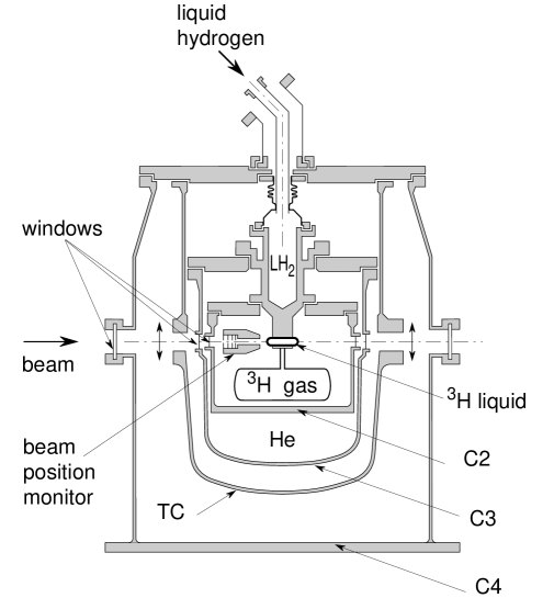
Figure 21: Saclay tritium target. The volume between containers C3 and C4 is filled with gaseous ${}^{4}He$ for a continuous check of integrity of C3 and C4. The volume C4 could retain the tritium at pressures below 1 bar.

The ${}^{3}H$-target proper consisted of a stainless steel cylinder, 40$mm$ long, 10$mm$ in diameter with hemispherical end caps located outside the acceptance of the spectrometer. The target was in permanent connection with an expansion-vessel of 180$cm^{3}$ volume. This vessel was equipped with a heater, in order to keep it at T $\sim$ 300K while the target was cold. When the entire system was at room temperature, the tritium pressure was 23 bars.

This combination of cold target and warm storage vessel had a number of outstanding benefits, such as high target density (liquid ${}^{3}H$), low operating pressure while the target was placed in the high-intensity electron beam (3 bars), very high efficiency in the use of the ${}^{3}H$ (98% in the cold target cell), well known density of liquid ${}^{3}H$, and thin target windows. Only 10kC of tritium were needed to reach the high target thickness.

Use of a liquid target with minimized amounts of ${}^{3}H$ involves a large amount of heavy nuclei (Cu, Fe) near the beam. A uranium collimator (diameter 8 $mm$) upstream of the target and outside the spectrometer acceptance eliminated potential stray electrons. A secondary emission monitor upstream of the target verified that no beam-halo was present. A split secondary emission monitor ensured stabilization of the beam position to 0.1 $mm$ accuracy.

For the extreme forward- and backward-angles (25^o and 155^o) the end caps of the target were not entirely outside the acceptance of the spectrometer. Insisting on this condition would have led to an undue increase of target length (i.e. quantity of ${}^{3}H$). For the extreme angle of 155^o — which is of great interest to the separation of $F_{ch}$ and $F_{m}$ — a special collimator placed close to the ${}^{3}H$ target eliminated all contributions from the end caps.

At the nominal temperature of 21.7K the target density was 0.2710$\pm$0.0014 $g/cm^{2}$. This led to a thickness of $\simeq$ 1 $g/cm^{2}$ at $\theta$ = 155^∘. With this large target thickness, data could be taken at momentum transfers where the cross section is very small. As a consequence, the region of the expected diffraction minimum and secondary maximum could be covered, and the experiment reached a maximum $q$ of 5.7$fm^{-1}$.

For ${}^{3}He$ the life of the experimentalist is somewhat easier, as no precautions due to radioactive gas are required; achieving an adequate target thickness still is a challenge.

Besides the experiments mentioned already above [193, 194] several groups have contributed to the ${}^{3}He$ data base. An experiment performed at Mainz by Ottermann et al. [198] provided data up to $q=1.9fm^{-1}$, lower-$q$ data were measured by Szalata et al. [199] and Dunn et al. [200].

The region of the diffraction minimum and secondary maximum of the charge form factor was first reached by the experiment of McCarthy et al. [201, 202] who, contrary to all other experiments, used a liquid target cooled to 1K using superfluid Helium. The diffraction feature in the magnetic form factor was reached in the experiment of Cavedon et al. [203].

The data on the charge form factor going to the largest $q$ were taken by Arnold et al. [204] in a coincidence experiment performed at SLAC. Due to the cryogenic target (42$cm$ of ${}^{3}He$ at 20K and 50 bar) a large target thickness was achieved, $\sim 5g/cm^{2}$. In combination with the high energy of $E_{e}$=15 GeV used — the cross section at a given $q$ is roughly proportional to $E_{e}^{2}$ — very small form factors (F $\sim 3\cdot 10^{-5}$) could be measured. This allowed Arnold et al. to reach a maximum momentum transfer of 10$fm^{-1}$, and cover the region of the second diffraction zero.

The form factors presently available, as extracted directly from the various experiments, are shown in fig. 22.

     

Figure 22: Charge and magnetic form factors of ${}^{3}He$.

An experiment performed at Bates [205] has produced two points at higher $q$ for magnetic scattering, the data have, however, not yet been published.

4.3 Experimental form factors

The world set of cross sections measured for ${}^{3}He$ and ${}^{3}H$ have been analyzed by Amroun et al. [197] in the same way as described in sect. 3.3 for the deuteron. The various form factors were parameterized using the SOG parameterization. From these form factors, the cross sections were calculated and the parameters fitted to the data. The separation of longitudinal and transverse form factors thereby was automatically achieved.

In order to analyze the electron scattering data it was assumed that the cross section can be expressed in the plane wave Born approximation (PWBA) as:

$$\sigma=\sigma_{Mott}\frac{1}{\eta}\left[\frac{q^{2}}{\vec{q}^{2}}F_{ch}^{2}(q)+\frac{\mu^{2}q^{2}}{2M^{2}}\left(\frac{1}{2}\frac{q^{2}}{\vec{q}^{2}}+tg^{2}\frac{\theta}{2}\right)F_{m}^{2}(q)\right]$$

where the Mott cross section contains the usual recoil and $Z^{2}$ factors, $\mu$ is the ${}^{3}H$(${}^{3}He$) magnetic moment, $\eta$ is given by $(1+q^{2}/4M_{T}^{2})$. $M$ ($M_{T}$) is the nucleon (three-nucleon) mass and $q$ ($\vec{q}$) is the four (three)-momentum transfer.

As the incident electron wave is distorted by the Coulomb field of the nucleus, the PWBA is not entirely valid. The DWBA form factors $F^{2}_{ch,DW}(E,\theta)$ and $F^{2}_{m,DW}(E,\theta)$ are related to the Born form factors $F^{2}_{ch}(q)$ and $F^{2}_{m}(q)$ by:

$$F^{2}_{ch}(q)=F^{2}_{ch,DW}(E,\theta)f_{c}(E,\theta),\hskip 56.9055ptF^{2}_{m}(q)=F^{2}_{m,DW}(E,\theta)f_{m}(E,\theta)$$

where $f_{c}$ and $f_{m}$ are Coulomb correction factors. Unfolding of these corrections allows to restore the PWBA formula and to infer the PWBA form factors that can be compared to theoretical predictions and will be used below.

Figure 23: Best fit charge form factors (curves with error band) and form factors derived using standard Rosenbluth plots in individual regions of $q$.

In order to unfold the Coulomb corrections from the experimental cross sections approximate charge and magnetization densities were used to compute the cross sections as a function of the actual energies and angles. This was done using a phase shift code for charge scattering [206], and the DWBA code HADES [207] for magnetic scattering. The Coulomb correction factors $f_{c},f_{m}$, obtained from the ratio of the exact to the PWBA cross sections, were found to be insensitive to the exact densities employed.

Amroun et al.  have also performed standard Rosenbluth separations of the data. As forward- and backward-angle data are not exactly at the same momentum transfer (although close as by now data at many angles are available), they have used the fit to shift the data to the $q$-value desired. At the $q$-value of interest the ratio $\sigma_{exp}/\sigma_{fit}$ of the neighbouring experimental $q$-value was used. The resulting $F_{ch}$ and $F_{m}$ agree with the ones from the global fit. The error bars are less precise, however, as for a determination at a given $q$ the global fit de facto uses the values of all data in the neighbouring $q$-interval; the width of this interval is given by $\sim 1/R_{max}\simeq 0.2fm^{-1}$.

In the paper of Amroun et al. [197] the best fit parameters for ${}^{3}H$ and ${}^{3}He$  are given together with the uncertainties of the form factors, so we dont need to repeat them here. (Note that eq.(1) contains a misprint, the numerical factor in the exponent should be 1/4 and not 1/2).

In fig. 23 the comparison between the global fit (curves with error band) and the form factors determined from Rosenbluth separations in individual intervals of $q$ is shown.

nucleus	type	$rms$-radius
${}^{3}H$	$C0$	1.755 $\pm$ 0.087 $fm$
${}^{3}H$	$M1$	1.840 $\pm$ 0.182 $fm$
${}^{3}He$	$C0$	1.959 $\pm$ 0.034 $fm$
${}^{3}He$	$M1$	1.965 $\pm$ 0.154 $fm$

On occasion, it is useful to know the $rms$-radii of the A=3 nuclei. They are listed in table 4.3, where the error bars given include both statistical and systematic uncertainties. For the magnetic form factors, the ”radii” given do not really correspond to a genuine radius; rather, they simply reflect the coefficient that occurs in the $q=0$ expansion of the magnetic form factor $F(q)=1-q^{2}r_{rms}^{2}/6+..$

4.4 Comparison to theory

As mentioned in sect. 2.3 a number of techniques are available to calculate the wave function starting from the (non-relativistic) Schrödinger equation and the known N-N interactions: Faddeev calculations in both coordinate- and momentum space [65, 66, 67, 208, 209, 210, 211, 212], the Correlated Hyperspherical Harmonics approach [71, 213] and Greens-function Monte Carlo methods [214]. Relativistic calculations are also becoming available [215, 216, 49, 217]. Calculations of the A=3 nuclei have been performed using the Blankenbecler-Sugar formalism [49] and the relativistic spectator (Gross) equation [217]. These relativistic calculations are of rather recent date, however, and the corresponding electromagnetic form factors have not yet been published.

In the following we first compare to the results of the recent calculation of Marcucci et al. [218]. These authors use the trinucleon wave functions calculated by Kievsky et al. [71] with the Pair-correlated Hyperspherical Harmonics (PHH) method. In this PHH calculation the AV18 N-N interaction, which includes charge-symmetry and charge-independence breaking terms and gives a very good fit to N-N scattering data, is used.

The AV18 force is complemented by the UIX three-body force which has a long-range part given by $2\pi$-exchange. At short range a phenomenological repulsive term is added to simulate dispersive effects. This part is fitted to the binding energies of the A=3, $\infty$ systems.

Figure 24: Contributions of different two-body charge terms, split into T=0 and T=1 components [218]. The one-body part is indicated by 1-N.

The two-body operators are calculated as discussed in sect. 2.4, i.e. they are consistently derived, as far as presently possible, from the N-N interaction employed. For the two-body currents the $\pi$- and $\rho$-like terms (PS and V in fig. 24) come from AV18. The model-dependent terms, $\pi\rho\gamma$ and $\omega\rho\gamma$, are calculated using known coupling constants and VDM form factors. The cut-off parameters needed at short range have been chosen to give a good description of the deuteron magnetic form factor $B(q)$ at high $q$. The three-body currents resulting from the $2\pi$-exchange in the 3BF employed is accounted for as well. For the two-body charge operators, which do depend on how the non-nucleonic degrees of freedom ($N\bar{N}$, $N^{*}$) have been eliminated from the wave function, the authors follow as much as possible the derivation of the corresponding $\pi$- and $\rho$-like terms in the two-body currents. Again the $\pi\rho\gamma$ and $\omega\rho\gamma$ terms have to be added separately. In fig. 24 the different contributions of the two-body charge terms are shown, split into their T=0 and T=1 components. It is obvious from the comparison to the one-body curve that two-body contributions will have an important effect upon the form factor in the region of the diffraction minimum and maximum.

Figure 25: A=3 charge form factors together with calculation of Marcucci et al. [218]. The IA result (dashed) , and the full result including two-body terms, is given.

Figure 26: A=3 magnetic form factors together with calculation of Marcucci et al. [218]. The IA result, the full result including two-body currents, and the result obtained when explicitly including $\Delta$’s are given.

Marcucci et al. have also explored the role of $\Delta$-components in the A=3 ground state. Often these degrees of freedom are included via the two-body currents, but a different picture might result once they are explicitly allowed for in the wave function, such as done previously by the group of Sauer [219, 220]. Marcucci et al. do not carry out a full coupled channel N-$\Delta$ calculation. Rather, they use the Transition Correlator Operator (TCO) method [221], which has proven to be useful in earlier variational calculations. In this case, they use the AV28Q N-N interaction which allows for both nucleons and Deltas.

In figs. 25,26 we show the comparison between the experimental results of the A=3 form factors and the predictions of Marcucci et al.. In each case we show both the IA-prediction, and the full calculation including two-body and three-body currents. For the case of the magnetic form factors, the results obtained by explicitly including the $\Delta$ in the wave function are also shown.

One observes that for all form factors the effect of two-body currents is quite important. In general, the full calculation does a very good job in explaining the data. The effect of explicitly including the $\Delta$ is rather small, significantly smaller than what was found by Strueve et al. [220], partly because different coupling constants were employed.

Figure 27: A=3 charge form factors together with calculations of Schiavilla et al. [222, 223] and Sauer and collaborators [220, 219].

Figure 28: A=3 magnetic form factors together with calculations of Schiavilla et al. [222, 223], Sauer and collaborators [220, 219] and Golak et al. [224].

In figs. 27,28 we compare the experimental data with further calculations of refs.[219, 220, 222, 223, 224], which also are based on nucleonic degrees of freedom.

Sauer and collaborators [219, 220] have solved the coupled-channel N-$\Delta$ Faddeev equations in momentum space, and used the Paris NN potential modified [219] to include $\Delta$-isobar excitations via $\pi$- and $\rho$-meson exchanges. The presence of the $\Delta$ thus accounts for the most important part of the three-body force. In this calculation $\pi$-, $\rho$-, and $\rho\gamma\pi$-meson exchange current contributions are included as well as the one-body Darwin-Foldy term and spin-orbit relativistic corrections. As for the calculation of ref. [218] boost corrections are not yet included.

Schiavilla and collaborators [222, 223] based their (older) calculation on a variational three-body wave function computed using the Argonne V14 interaction and the Urbana-VII three-nucleon force. In this calculation the $\pi$-like and $\rho$-like meson exchange currents were derived consistently from the NN interaction used. The authors also included the one-body relativistic corrections mentioned above as well as $\omega$-exchange and $\omega\gamma\rho$-contributions.

Golak et al. [224] in their recent calculation solve the Faddeev equations in momentum space, using the AV18 N-N potential. The two-body currents, which up to now are only calculated for the magnetic form factors, are treated according to ref. [225].

For all calculations the two-body terms significantly displace the diffraction minimum of the charge form factors to lower $q$ values and increase the height of the secondary maximum by more than a factor of two. The calculations achieve a similarly good agreement with ${}^{3}H$. This is not the case for ${}^{3}He$ where ref. [220] slightly underestimates the charge form factor, whereas the calculation of ref. [222] almost perfectly agrees with it. The difference could be due to the model dependence of the one-body term, or due to different two-body contributions. Indeed, for the ${}^{3}H$ form factor, the calculations of refs. [220] and [223] predict the one-body minimum at 3.9 and 4.15$fm^{-1}$ respectively, while the predictions for the full calculation perfectly agree. Additional differences might come from the different parameterizations of the nucleon form factors used, particularly for the poorly known G_en. We do not understand why the ${}^{3}H$ form factors are better predicted than the ones for ${}^{3}He$.

For the magnetic form factors, where the effect of the three-body force is also quite small, the effect of the two-body currents is larger than for the charge form factor, and they improve considerably the agreement with experiment. However, none of the calculations perfectly accounts for the shape of the ${}^{3}He$ form factor: the prediction of ref. [219] explains its shape below the diffraction minimum, but fails above, whereas ref. [222] shows the opposite behaviour. The latter calculation agrees with the ${}^{3}H$ form factor, while this is not the case for ref. [219].

There are several differences between these two calculations. As for the charge form factors they differently predict the one-body contribution. The IA predictions for the location of the diffraction minima of ${}^{3}H$ are 3.5 and 3.7 $fm^{-1}$ for the calculations of Sauer and Schiavilla, respectively. The differences in the exchange current contribution are even larger.

While qualitatively the role of two-body currents is understood, the situation for the magnetic form factors in particular is not yet entirely satisfactory when it comes to a quantitative comparison. Even at low $q$, some differences between experiment and theory remain. While experimentally the ${}^{3}H$ (${}^{3}He$) magnetic moments amount to 2.98 (–2.13) $\mu_{N}$, the theoretical predictions are e.g. 2.98 (–2.09) for V₁₈ and 2.87(–2.06) for the Paris interaction.

Fig. 29 shows, for completeness, the isospin-separated $A=3$ charge form factors together with the theoretical predictions of Strueve et al. and Marcucci et al. [220, 218]. The main observation from these comparisons is that the T=0 charge form factor is remarkably well predicted by both calculations. This agreement is quite unexpected since it is reached after adding ”model-dependent” two-body contributions, which lead to a sizeable change. For the T=1 charge form factor we observe larger differences between the theoretical predictions. Moreover, none of them perfectly describes the data. Since the agreement for the T=0 component has been found to be excellent for all of them, we conclude that improvement in the description of the trinucleon requires improvement of the calculation of its isovector charge component.

Figure 29: T=0 and T=1 charge form factors of the A=3 systems, compared to the calculations of Marcucci et al. [218] (solid) and Strueve et al. [220] (dashed).

For the T=0,1 magnetic form factors the calculations are closer to the data, so we do not separately show them.

4.5 A=2,3 comparison

In order to understand better whether eventual shortcomings in our understanding of the 3N-systems are only related to the two-body input, or whether our understanding of genuine three-body properties is lacking, it is of interest to directly compare the 2- and 3-body form factors.

To achieve this, one can extract from the ${}^{3}He$ and ${}^{3}H$ form factors the corresponding isoscalar- and isovector quantities, where the former then is directly comparable to the deuteron form factor. This comparison becomes particularly interesting now that the diffraction structure of the A=2 $C0$ charge form factor is well determined.

The isoscalar $F_{T=0}$ and isovector $F_{T=1}$ components of the A=3 charge form factors are defined by the following expressions:

$$F_{0}(q)=\frac{1}{2}\left[2F_{He}(q)+F_{H}(q)\right]\hskip 28.45274ptF_{1}(q)=\frac{1}{2}\left[2F_{He}(q)-F_{H}(q)\right]$$

and similarly for the magnetic form factors:

$$F_{0}(q)=\frac{1}{2}\left[\mu_{He}F_{He}(q)+\mu_{H}F_{H}(q)\right]\hskip 28.45274ptF_{1}(q)=\frac{1}{2}\left[\mu_{He}F_{He}(q)-\mu_{H}F_{H}(q)\right]$$

where $\mu_{H}$ and $\mu_{He}$ are the A=3 magnetic moments and all ${}^{3}He$ and ${}^{3}H$  form factors are normalized to 1 at $q=0$. The T=0,1 form factors can easily be calculated from the parameters of the ${}^{3}He$ and ${}^{3}H$ form factors [197]. The effect of the isospin impurity, due to the Coulomb interaction in ${}^{3}He$, has been neglected. Indeed, its effect on the ${}^{3}He$  charge form factor is very small, $\leq 1\%$ in the region of the secondary diffraction maximum and even smaller for lower $q$ values.

Figure 30: Correlation between the position of the diffraction minima in the A=2 and A=3 isoscalar charge form factors (top) and the amplitudes of the form factors in the diffraction maxima (bottom). The experimental point is indicated by the shaded area (exp).

Henning et al. [155] have made a detailed comparison between some of the global properties of the A=2,3 charge form factors such as the position of the diffraction minima, the position of the maxima and the amplitude of the form factors in the maxima. They have done so by calculating the A=2,3 form factors for a number of N-N interactions, with and without inclusion of the two-body currents. The potentials employed were the venerable RSC potential, the Paris potential and various OBE Bonn potentials OBEPQ, OBEPA,OBEPB and OBEPC.

It turns out that the above-mentioned observables display a remarkable correlation between the A=2 and A=3 systems. There is a basically linear relationship between the A=2 and A=3 quantities. This is demonstrated in fig. 30 which gives the amplitude of the A=3 isoscalar charge form factor in the diffraction maximum as a function of the same quantity for the deuteron. Not only do the values for the different potentials (to which we have added the AV18 potential) define a basically linear correlation, the points with/without two-body currents also lie on the same line. Within the line, there is a correlation between the strength of the tensor interaction and the position of the minimum: N-N potentials yielding a larger D-state produce a minimum at lower $q$. The lower part of the figure gives the corresponding relation between the positions of the diffraction zeroes.

The inclusion of the AV18 points shows that this line is rather general; it is not simply a consequence of the particular way the two-body contributions are calculated. There is some qualitative understanding for the occurrence of this correlation [155]: if the A=3 nuclei could be described in a quasi-deuteron model, such a correlation would be expected. A quasi-deuteron model is obviously much too primitive for the A=3 system, but the three-nucleon wave functions obtained from the Faddeev equations do approximately show the symmetry upon interchange of the Jacobi momenta $p$ and $\sqrt{3}/2q$ which would result from the spectator model.

The non-understood feature of fig. 30 lies in the fact that the line describing all theoretical calculations does not pass through the experimental point indicated by ”exp”, particularly for the amplitudes in the diffraction maxima. From the comparison with experiment it would seem that the existing range of non-relativistic N-N potentials together with the present understanding of two-body currents is not able to account simultaneously for the properties of the A = 2,3 systems.

Besides the difficulties with the ${}^{3}He$ magnetic form factor, the discrepancy shown in fig. 30 is one of the major open problems, and potentially points to the need to go beyond the ”nuclear standard model”.

5 Helium-4

The four-body system is interesting as the $\alpha$-particle is tightly bound, and the nucleons are dominantly in a spatially symmetric S-state configuration. As a consequence, a high central density (the highest in nuclei) is found in ${}^{4}He$.

The data base for the ${}^{4}He$ charge form factor is reasonably complete, and the form factor measurements extend to unusually large $q$. The pioneering experiment was performed by R. Frosch et al. at Stanford [226] using a liquid helium target. This experiment already reached the diffraction maximum at $4fm^{-1}$.

More precise data at medium momentum transfers were provided by an experiment carried out also at the Stanford HEPL by McCarthy et al. [202]; this experiment focused on the ${}^{3}He$ form factors, the ${}^{4}He$ was measured mainly as a check. The separation of longitudinal and transverse contributions, necessary for ${}^{3}He$, was performed for ${}^{4}He$ as well, in order to certify that indeed a transverse form factor compatible with zero was found for ${}^{4}He$. As the systematic errors are very different for the forward angle (high energy) and backward angle (low energy) data, this provided a very stringent and useful test of the quality of the data.

Data at very low $q$ are also available from the experiment of Erich et al. [227] performed at the Darmstadt electron accelerator. This experiment used a mixed H/He gas target in order to obtain a continuous normalization of the helium cross sections relative to the proton. Low-$q$ data were also measured by Ottermann et al. [198] at Mainz, using a 14bar gas target, collimated to exclude the contribution of the target windows.

The highest momentum transfers were achieved by an experiment carried out at SLAC by Arnold et al. [204]. In this experiment, which used electron energies up to 15GeV, a long gas target at 20K and 50 bar was used to obtain a high target thickness and large luminosity. Due to the high electron energy and the correspondingly poor energy resolution, the scattered electron and recoil helium had to be detected in coincidence using the 20GeV/c and 8GeV/c-spectrometers. The measurements reached a momentum transfer of 8$fm^{-1}$, where the count rates dropped to 1 event/week; the steepness of the fall-off of the form factor at the highest $q$ is indicative of the presence of a second diffraction zero.

For ${}^{4}He$, as for the other few-body nuclei discussed in this review, we have used the world data to determine the experimental form factor. The treatment of the data and their uncertainties is similar to what was discussed for the case of the A=2,3 systems. The resulting form factors are shown below in the figures.

Several groups have calculated the ground-state wave function of the 4-body system. As for the A=3 nuclei, ${}^{4}He$ is underbound by several $MeV$ in calculations that only include two-body forces. The contribution of a three-body force must be added. As a matter of fact, the ${}^{4}He$ binding energy is often used to fix the scale factor of this 3-body force.

Glöckle and collaborators [228, 229] have employed the Faddeev-Yakubovsky technique using a selection of N-N interactions, Viviani et al. [213] have employed the Correlated Hyperspherical Harmonics (CHH) approach together with the AV14 and AV14+TNI8 interactions. As far as ground-state properties such as binding energies go, these calculations compare well to the Variational Monte Carlo (VMC) results obtained by Arriaga et al. [230] and the Greens-Function Monte Carlo results of Carlson and Schiavilla [231, 232].

Further results for the ${}^{4}He$ charge form factor are available from Schiavilla et al. [223] based on a VMC calculation using the Argonne V14 potential supplemented by the Urbana VII three-nucleon interaction. The most recent result has been obtained by Schiavilla and Carlson using the V18 potential supplemented by the Urbana IX three-nucleon interaction [233].

Figure 31: Experimental form factor of ${}^{4}He$ together with IA (dashed) and full calculation of Carlson and Schiavilla [233] performed using the Argonne V18 N-N potential together with the Urbana IX three-body force.

In fig. 31 we show the results of the latest calculation together with the IA-prediction. The figure shows that modern calculations do extremely well in reproducing the experimental data. The effect of the two-body terms is very important in achieving this good agreement, particularly for the height of the diffraction maximum at $4fm^{-1}$. This is the case despite the less than satisfactory state of the theory of isoscalar two-body contributions for the charge form factor. When comparing the isoscalar charge form factors of A=3 [197] and A=4 one notes that in both cases theory somewhat overpredicts the form factor in the diffraction maximum.

The breakdown of the different contributions to the two-body terms is given in fig. 12 of ref. [223]. The individual contributions are quite similar to what we have shown in fig. 24 for the isoscalar A=3 form factor. The $\pi$-like (PS) and $\rho$-like terms (V) give the largest contribution at high momentum transfer. The single-nucleon relativistic correction, the Darwin-Foldy (DF) and Spin-Orbit (SO) terms are also significant at large $q$, and help to get large enough a (absolute value of the) form factor in the diffraction maximum. The contribution of the most model-dependent two-body terms fortunately is relatively small.

In order to show the progress of the understanding of the ${}^{4}He$ form factor, fig. 32 displays the result of an early calculation by Gari et al. [234]. This calculation was performed using the exp(S)-approach, including up to 4-particle correlations. The curve shown was calculated using the RSC N-N interaction together with a phenomenological three-body force. The two-body contributions were calculated according to the approach by Gari and Hyuga [148]. The main discrepancy to the data occurred in the region of the diffraction maximum. The comparison to modern calculations (fig. 31) shows that both the IA contribution and the two-body contributions have increased by nearly a factor of 2, due to both a better ground-state wave function and a more consistent calculation of the two-body processes.

Figure 32: Experimental ${}^{4}He$ form factor together with early results from the exp(S)-calculation of Gari et al. [234] (solid curve) and the VMC calculation of Schiavilla et al. [223] performed using the V14 interaction (dashed).

In fig. 32 we also show the results of an older calculation of Schiavilla et al.  [223] obtained using the Argonne V14 plus Urbana-VII TNI interactions. A similar observation can be made for this calculation.

The data have also been used by Sick [235] to determine an accurate charge radius, with the goal to compare it to a precise measurement from the 2p-2s transition in muonic helium by Carboni et al. [236]. For ${}^{4}He$ such an analysis can be done by including information from other observables on the large-radius behaviour of the proton radial wave function. This large-$r$ behaviour has a considerable influence on the rms-radius, but is not very well determined by electron scattering as at small $q$, where its effect shows up, the experimentally determined signal, the difference of the form factor to one, becomes small and affected by systematic errors.

For ${}^{4}He$ the shape of the proton radial wave function is calculable knowing the proton separation energy. The absolute normalization is known from a dispersion-relation analysis [237] of the world-data on proton-helium elastic scattering. This constraint helps to extract from the (e,e) data a very precise charge rms-radius, 1.676 $\pm$ 0.008 $fm$, which agrees with the value measured using muonic atoms.

The calculation corresponding to fig. 31 of Schiavilla et al. [233] gives a charge radius of ${}^{4}He$ of 1.609 $fm$. Once the contribution of two-body currents is added, this increases to 1.634 $fm$. In comparison with the experimental result, this is a bit low.

Overall, the understanding of the ${}^{4}He$ form factors is quite satisfactory. This shows that the calculations of the isoscalar two-body contributions are quite successful even in dense systems, although the theoretical understanding of these terms still leaves to be desired. Other open questions on the structure of ${}^{4}He$, such as the size of the D-state contribution or the role played by ${}^{1}S_{0}$ vs ${}^{3}S_{1}$ pairing, are better investigated by studying breakup observables.

6 A$>$4

The region of ”light nuclei” up to a few years ago certainly did not go beyond mass number A=4: for heavier nuclei calculations of accuracy comparable to A$\leq$4 could not be performed. In this situation, one had to take recourse to more approximate, and much less fundamental, approaches such as the shell model, cluster models etc. Some of these calculations have reached quite a high standard (see e.g.[238]), but these approaches do not provide the direct link to the underlying N-N interaction.

This situation has changed during the last years. Today, Greens-Function Monte Carlo (GFMC) calculations can be performed for nuclei up to mass A=9 [64, 76], and Variational Monte Carlo (VMC) calculations have been performed up to A=16 [92, 239, 240]. A recent exp(S)-calculation also reaches A=16 [241]. In these calculations, the nuclear wave function can be obtained starting from the N-N interaction, with no additional model assumptions. Despite the daunting numerical effort required and some approximations that do have to be made, the results seem to indicate that a fairly accurate understanding is being reached for these not-so-light nuclei.

It is of great interest to study the p-shell nuclei in terms of ”exact” methods. For the heavier p-shell nuclei, at least, the shell model already provides a reasonable description; in this case the comparison between the ”exact” calculations and the model-calculations allows us to assess the accuracy and potential failures of the latter, and herewith lets us gain most valuable insight needed when dealing with even heavier nuclei where ”exact” calculations are out of question for quite some time to come.

GFMC calculations for nuclei up to A=9 have been performed by Pudliner et al. [64, 76]. These calculations employed the AV18 N-N interaction together with the Urbana IX three-body force. For the binding energies, these calculations reach accuracies of the order of 1$MeV$ out of 40$MeV$. The calculations show that the N-N correlations continue to play an important role even for the heavier nuclei; the two-body densities for these heavier nuclei actually at N-N distances $<2~{}fm$ are quite similar to the ones found for the deuteron.

Figure 33: ⁶Li form factors calculated by VMC by Wiringa and Schiavilla ($\circ$) [242] together with data for C0+C2 [243, 244] and M1 [245, 246, 247] (+).

Only for some of the p-shell nuclei and selected states have the electromagnetic form factors been calculated. In these calculations the two-body currents have been included in the way discussed in sect. 2.4, i.e. as far as possible consistently with the underlying N-N interaction. In figs. 33,34 we show two examples. For the ${}^{6}Li$ charge form factor the results calculated using VMC agree quite well with the data of G.C. Li et al. [243] measured at Stanford, and Bumiller et al. [244] and Suelzle et al. [248] at the lower momentum transfers. The calculations include the contributions from two-body currents which have an effect only near the diffraction minimum where they shift it to somewhat smaller $q$. Both the data and the calculation correspond to the sum of the $C0$ and $C2$ multipolarities (${}^{6}Li$ has spin one) which have not been separated. The agreement between calculated (2.59$\pm$0.02$fm$) and experimental (2.56$\pm$0.05$fm$) charge rms-radius is quite good.

The magnetic form factor of ${}^{6}Li$ has first been measured by Rand et al. [245]; the 180^∘ degree data, which reach 1.4$fm^{-1}$, still had large statistical errors. Precise data were obtained by Lapikas et al. [246] at low $q$, and Bergstrom et al. [247] by an experiment performed using the 180^∘ setup at Bates. The ${}^{6}Li$ magnetic form factor calculated by Wiringa and Schiavilla, displayed in fig. 33b, does not show as good an agreement with the data for momentum transfers $q>1fm^{-1}$. This discrepancy with the data is not due to two-body currents, which have a relatively minor effect as ${}^{6}Li$ is an isoscalar system; one therefore must assume that it is related to deficiencies in the VMC wave function.

Figure 34: $Exp(S)$ calculation of the oxygen effective form factor ($\sigma/\sigma_{Mott}$) by Mihaila and Heisenberg [241], compared to the data of Sick and McCarthy [249] and Bentz [250].

For Oxygen, Mihaila and Heisenberg [241] have recently used the $exp(S)$ coupled-cluster expansion approach. The procedure is similar to the $exp(S)$ method used at the time by Gari et al. [148] (see fig. 32) who, in addition to ${}^{4}He$, also considered heavier magic nuclei such as oxygen and calcium. In the coupled cluster approach, the nuclear wave function is expanded in the many-body Hilbert space in terms of multiconfigurational creation- and destruction operators. The expansion coefficients carry the information on the nuclear correlations, and no distinction between short- and long-range correlation needs to be made. The wave function is expanded in a 50$\hbar\omega$ space, and relative angular momenta up to l=11 are taken into account. In this calculation, the Argonne V18 N-N interaction together with the Urbana IX three-body force is employed. Two-body currents are also included, and have a moderate effect at momentum transfers above 2 $fm^{-1}$. The Coulomb distortion is accounted for by Fourier-transforming the calculated form factor to $r$-space, and then calculating the Coulomb-distorted cross section (effective form factor) using a phase-shift code.

The calculation is compared in fig. 34 to data [249] obtained in an experiment that used a windowless ice-target at LN₂ temperature. The low-$q$ data (0.3 – 0.5 $fm^{-1}$) have been measured at Darmstadt by Bentz [250].

The agreement between calculation and experiment is amazingly good. In $r$-space, somewhat larger deviations are visible as the calculated $rms$-radius of 2.62$fm$ [251] is smaller than the experimental one of 2.712$\pm$0.005$fm$. It will be interesting to see whether this $exp(S)$ approach of Mihaila and Heisenberg can with similar success predict the properties of other p-shell nuclei.

7 Conclusions and outlook

In this paper we have reviewed the present status of the elastic form factors of nuclei with mass number A=2,3,4,6 and 16, both in terms of the cross section data available, the form factors extracted and their theoretical understanding. For the case of the deuteron, we have included the transition form factor to the singlet-S state.

We have witnessed during the last years important progress in the theory used to calculate few-body wave functions and the corresponding electromagnetic form factors. The ”nuclear standard model” — based on the assumption that nuclei are basically non-relativistic systems containing nucleons bound by the N-N interaction known from N-N scattering — is surprisingly successful. For the nuclei where the computational techniques are well under control, basically $A\leq 4$, the agreement between calculated ground state properties, and form factors in particular, is very satisfactory.

The most important uncertainties for $A\leq 4$ still result from the poorly constrained nature of the N-N interaction off-shell. There, different N-N potentials give quite different answers. The ensuing differences mainly affect D-state properties. The same quantities are somewhat uncertain as the data base that fixes the S-D transition in the NN-system, represented by the $\epsilon_{1}$-parameter, is still not very satisfactory and leaves too much freedom for the N-N potentials. Here, only double-polarization experiments on $\vec{n}-\vec{p}$ elastic scattering can be expected to lead to significant progress in the future.

For the calculation of the electromagnetic form factors, it also has been very important to get the contributions of two-body terms, required by gauge invariance, under control. Much progress in this direction has been made, as many of the two-body terms now can be derived consistently with the N-N interaction employed. Diagrams not constrained by current conservation occasionally still involve significant uncertainties, though.

One obvious avenue for a deeper understanding of light nuclei consist in a relativistic treatment. Given the typical momenta of nucleons in nuclei, a relativistic description is clearly desirable. A number of different approaches have been developed already, and we have addressed some of them when discussing the deuteron. For the heavier systems, the covariant calculations up to now have provided little in terms of form factors, the quantities that yield the perhaps most detailed test. The covariant approaches also give us a better control over the off-shell behaviour and thus have the potential to partly do away with one ingredient of the non-relativistic calculations that still is somewhat unsatisfactory, the (phenomenological) three-body interaction. In this area, significant advances can be expected during the coming years.

On the side of experiment, good progress has also been made. In particular, we now have a reasonably complete set of polarization data for electron-deuteron scattering that allows us to separate the deuteron monopole- and quadrupole form factors. For a long time, we had to contend with the unseparated structure function $A(q)$, which is much less sensitive to the underlying physics.

In this review, we have used for the nuclei A=2–4 the form factors resulting from a fit to the world data, such as to base the discussion on the most precise experimental information presently available. The numerical values of the various form factors, which partly have been determined in the course of writing this review, are available upon request.

While our knowledge of the proton charge- and the neutron magnetic form factors has greatly improved during the last years, the neutron charge form factor $G_{en}$ remains a continued source of uncertainty for the understanding of few-body charge form factors. The first double-polarization experiments now have produced results and lead to values of $G_{en}$ that are more reliable than what was available up to now, but the uncertainties on $G_{en}$ are still comparatively large, and the information is limited to moderate values of the momentum transfer. Here, important further progress is required in the future. With the CW-facilities today available and the progress in polarized target and polarimeter design, the necessary improvements are within reach.

As far as the heavier nuclei go, it is very satisfactory to see the emergence of ”exact” calculations (in the sense of the nuclear standard model) for p-shell nuclei. In the p-shell, these calculations can be used to ”calibrate” the mean-field calculations that are standard (and often the only feasible ones) for heavier nuclei.

When looking at the overall comparison of theory and experiment, a few notable discrepancies remain. Even the most modern calculations do not very well describe the ${}^{3}He$ magnetic form factor; the reason for this is not known and cannot easily be blamed on the two-body contributions which for this observable are largely of the model-independent kind. The comparison between the positions of the minima, and amplitudes of the form factor maxima, for the A=2,3 systems also shows a persistent discrepancy. It is not clear if this can be taken as a signal for ”new physics” beyond the nuclear standard model. It is worrisome as well that the calculations do not yet accurately explain the static properties ($Q,\mu$) of the simplest nucleus, the deuteron.

It would evidently be of great interest to go to larger momentum transfer for some of the form factors. An extension of the ${}^{3}He$ magnetic form factor to larger $q$ will be carried out at JLAB, a significant extension for the two Tritium form factors is clearly feasible with available liquid-target technology. Pushing the $T_{20}$ measurements for the deuteron to higher $q$ will presumably require the development of a more efficient polarimeter of as yet unknown type.

Several aspects have received little attention in this review. Changes of the nucleon upon integration in the nucleus have not been discussed, essentially because there is little experimental evidence for it. We have also only occasionally discussed an understanding of the light nuclei in terms of quark constituents; the description in terms of nucleons is very successful, and clear signals for the need of a description in terms of the underlying quark degrees of freedom are hardly available. These signals probably only can be found by going to larger momentum transfers where the conventional description of light nuclei in terms of nucleonic constituents interacting via the N-N force must break down.
Acknowledgements
Many people have contributed to this review. We want to thank in particular H. Arenhövel, J. Carlson, T.W. Donnelly, J. Golak, H. Henning, J. Jourdan, D. Rohe, P. Sauer, R. Schiavilla, W. VanOrden and R. Wiringa who have provided help, advice or numerical results. This work was supported by the Schweizerische Nationalfonds.

References

- [1] T. deForest and J.D. Walecka. Adv. Phys., 15:1, 1966.
- [2] T.W. Donnelly and Ingo Sick. Review of Modern Physics, 56:461, 1984.
- [3] B. Frois. Edts. B. Frois, I. Sick, World Scientific, 1991.
- [4] R.G. Sachs. Phys. Rev., 126:2256, 1962.
- [5] G. Hoehler, E. Pietarinen, I. Sabba-Stefanescu, F. Borkowski, G.G. Simon, V.H. Walther, and R.D. Wendling. Nucl. Phys. B, 114:505, 1976.
- [6] P. Mergell, U.G. Meissner, and D. Drechsel. Nucl. Phys. A, 596:367, 1996.
- [7] F. Iachello, A.D. Jackson, and A. Lande. Phys. Lett., 43B:191, 1973.
- [8] M. Gari and W. Krümpelmann. Phys. Lett. B, 173:10, 1986.
- [9] M.K. Jones et al. Phys. Rev. Lett., 84:1398, 2000.
- [10] Th. Popischill et al. Eur. Phys. J. C, to be publ.
- [11] B.D. Milbrath, J.I. McIntyre, C.S. Armstrong, D.H. Barkhuff, W.Bertozzi, D. Dale, G. Dodson, K.A. Dow, M.B. Epstein, M. Farkhondeh, J.M. Finn, S. Gilad, M.K. Jones, K. Joo, J.J. Kelly, S. Kowalski, R.W. Lourie, R. Madey, D.J. Margaziotis, P. Markowitz, C. Mertz, J. Mitchell, C.F. Perdrisat, V. Punjabi, L. Qin, P.M. Rutt, A.J. Sarty, D. Tieger, C. Tschalaer, W. Turchinetz, P.E. Ulmer, S.P. Van Verst, G.A. Warren, L.B. Weinstein, and R.J. Woo. Phys. Rev. Lett., 80:452, 1998.
- [12] J. Jourdan. Workshop on Electron-Nucleus Scattering, eds. O. Benhar, A. Fabrocini, Edizioni ETS, Pisa, page 13, 1997.
- [13] H. Anklin, E.E.W. Bruins, D. Day, D. Fritschi, B. Groft, F.C.P. Joosse, J. Jourdan, J. Lichtenstadt, M. Loppacher, G. Masson, J. Mitchell, I. Sick, and H.J.J. vanVeen. Phys. Lett. B, 336:313, 1994.
- [14] H. Anklin, L.J. de Bever, S. Buttazzoni, A. Honegger, J. Jourdan, G. Kubon, T. Petitjean, L.M. Qin, I. Sick, Ph. Steiner, M. Zeier, J. Zhao, B. Zihlmann, J. Golak, H. Witała, W. Glöckle, and H. Kamada. Nucl. Phys. A, 636:189, 1998.
- [15] J. Jourdan. Nucl. Phys. A, 689:425, 2001.
- [16] W. Xu et al. Phys. Rev. Lett., 85:2900, 2000.
- [17] H. Gao et al. Phys. Rev. C, 50:R546, 1994.
- [18] E.E.W. Bruins, Th.S. Bauer, H.W. den Bok, C.P. Duif, W.C. van Hoek, D.J.J. de Lange, A. Misiejuk, Z. Papandreou, E.P. Sichtermann, J.A. Tjon, H.W. Willering, D.M. Yeomans, H. Reike, D. Durek, F. Frommberger, R. Gothe, D. Jakob, G. Kranefeld, C. Kunz, N. Leiendecker, G. Pfeiffer, H. Putsch, T. Reichelt, B. Schoch, D. Wacker, D. Wehrmeister, M. Wilhelm, E. Jans, J. Konijn, R. de Vries, C. Furget, E. Voutier, and H. Arenhövel. Phys. Rev. Lett., 75:21, 1995.
- [19] P. Markowitz, J.M. Finn, B.D. Anderson, H. Arenhoevel, A.R. Baldwin, D. Barkhuff, K.B. Beard, W. Bertozzi, J.M. Cameron, C.C. Chang, G.W. Dodson, K. Dow, T. Eden, M. Farkhondeh, B. Flanders, C. Hyde-Wright, W.-D. Jiang, D. Keane, J.J. Kelly, W. Korsch, S. Kowalski, R. Lourie, R. Madey, D.M. Manley, J. Mougey, B. Ni, T. Payerle, P. Pella, T. Reichelt, P.M. Rutt, M. Spraker, D. Tieger, W. Turchinetz, P.E. Ulmer, S. Van Verst, J.W. Watson, L.B. Weinstein, R.R. Whitney, and W.M. Zhang. Phys. Rev. C, 48:R5, 1993.
- [20] J. Jourdan, I. Sick, and J. Zhao. Phys. Rev. Lett., 79:5186, 1997.
- [21] G.P. Kubon. PhD thesis, University of Basel, 1999.
- [22] A. Lung et al. Phys. Rev. Lett., 70:718, 1993.
- [23] S. Kopecki, J.A. Harvey, N.W. Hill, M. Krenn, and M. Pernicka. Phys. Rev. C, 56:2229, 1997.
- [24] M. Gari and W. Krümpelmann. Phys. Lett. B, 274:159, 1992.
- [25] R.A. Brandenburg and P.U. Sauer. Phys. Rev. C, 12:1101, 1975.
- [26] S. Platchkov, A. Amroun, S. Auffret, J.M. Cavedon, P. Dreux, J. Duclos, B. Frois, D. Goutte, H. Hachemi, J. Martino, X.H. Phan, and I. Sick. Nucl. Phys. A, 510:740, 1990.
- [27] S. Galster, H. Klein, J. Moritz, K.H. Schmidt, D. Wegener, and J. Bleckwenn. Nucl. Phys. B, 32:221, 1971.
- [28] W. Plessas, V. Christian, and R.F. Wagenbrunn. Few Body Syst. Suppl., 9:429, 2000.
- [29] A. Buchmann, H. Henning, and P.U. Sauer. Few Body Syst., 21:149, 1996.
- [30] J. Carlson and R. Schiavilla. Rev. Mod. Phys., 70:743, 1998.
- [31] H. Arenhövel, F. Ritz, and T. Wilbois. Phys. Rev. C, 61:034002, 2000.
- [32] M. Meyerhoff et al. Phys. Lett. B, 327:201, 1994.
- [33] J. Becker. thesis, University of Mainz, 1997.
- [34] J. Becker et al. Eur. Phys. J. A, 6:329, 1999.
- [35] D. Rohe, P. Bartsch, D. Baumann, J. Becker, J. Bermuth, K. Bohinc, R. Bohm, S. Buttazoni, T. Caprano, N. Clawiter, A. Deninger, S. Derber, M. Ding, M. Distler, A. Ebbes, M./ Ebert, I. Ewald, J. Friedrich, M Kahrau, A. Klein, M. Kohl, K.W. Krygier, G. Kubon, A. Liesfels, H. Merkel, K. Merle, P. Merle, M. Mühlbauer, U. Müller, R. Neuhausen, E.W. Otten, Th. Petitjean, Th. Popischil, M. Potokar, G. Rosner, H. Schmieden, I. Sick, S. Sirca, R. Surkau, A. Wagner, Th. Walcher, G. Warren, M. Weis, H. Woehrle, and M. Zeier. Phys. Rev. Lett., 83:4257, 1999.
- [36] C. Herberg et al. Eur. Phys. J. A, 5:131, 1999.
- [37] T. Eden et al. Phys. Rev. C, 50:R1749, 1994.
- [38] M. Ostrick et al. Phys. Rev. Lett., 83:276, 1999.
- [39] I. Passchier et al. Phys. Rev. Lett., 82:4988, 1999.
- [40] H. Zhu, A. Ahmidouch, H. Anklin, C. Armstrong, C. Bernet, W. Boeglin, H. Breuer, D. Brown, S. Bueltmann, R. Carlini, N. Chant, A. Cowley, D. Crabb, S. Danagoulian, D. Day, T. Eden, R. Ent, Y. Farah, K. Garrow, C. Harris, M. Hauger, A. Honegger, R. Hutchins, M. Kaufmann, M. Khandaker G. Kubon, J. Jourdan, J. Lichtenstadt, R. Lindgren, A. Lung, D. Mack, S. Malik, P. Markowitz, K. McFarlane, P. McKee, D. McNulty, G. Milanovich, J. Mitchell, H. Mkrtchyan, M. Muehlbauer, T. Petitjean, Y. Prok, D. Rohe, E. Rollinde, O. Rondon, P. Roos, R. Sawafta, I. Sick, C. Smith, T. Southern, M. Steinacher, S. Stepanyan, V. Tadevosyan, R. Tieulent, A. Tobias, W. Vulcan, G. Warren, H. Woehrle, S. Wood, C. Yan, M. Zeier, J. Zhao, H. Zhu, and B. Zihlmann. Phys. Rev. Lett., 87:081801, 2001.
- [41] R. Machleidt. Adv. in Nucl. Phys., 19:189, 1989.
- [42] R. Machleidt and Q.G. Li. Phys. Rep., 242:5, 1994.
- [43] R.R.V.Reid. Annals of Physics, 50:411, 1968.
- [44] W.N. Cottingham, M. Lacombe, B. Loiseau, J.M. Richard, and R. VinhMau. Phys. Rev. D, 8:800, 1973.
- [45] M.M. Nagels, T.A. Rijken, and J.J. de Swart. Phys. Rev. D, 17:768, 1978.
- [46] R.B. Wiringa, R.A. Smith, and T.L. Ainsworth. Phys. Rev. C, 29:1207, 1984.
- [47] R.B. Wiringa, V.G.J. Stoks, and R. Schiavilla. Phys. Rev. C, 51:38, 1995.
- [48] V.G.J. Stoks, R.A.M. Klomp, and C.P.F. Terheggen. Phys. Rev. C, 49:2950, 1994.
- [49] R. Machleidt, F. Sammarruca, and Y. Song. Phys. Rev. C, 53:1483, 1996.
- [50] V.G.J. Stoks, R.A.M. Klomp, M.C.M. Rentmeester, and J.J. deSwart. Phys. Rev. C, 48:792, 1993.
- [51] M. Lacombe, B. Loiseau, J.M. Richard, R. Vinh Mau, J. Côté, P. Pires, and R. deTourreil. Phys. Rev. C, 21:861, 1980.
- [52] R. Machleidt, K. Holinde, and Ch. Elsters. Phys. Rep., 149:1 and 373, 1987.
- [53] D.V. Bugg and R.A. Bryan. Nucl. Phys. A, 540:449, 1992.
- [54] R. Henneck. Phys. Rev. C., 47:1859, 1993.
- [55] R.A. Arndt, R.L. Workman, and M.M. Pavan. Phys. Rev. C, 49:2729, 1994.
- [56] M. Ockenfels, F. Meyer, T. Köble, W. vonWitsch, J. Weltzle, K. Wingender, and G. Wollmann. Nucl. Phys. A, 534:248, 1991.
- [57] J. Fujita and H. Miyazawa. Prog. Theo. Phys., 17:360, 1957.
- [58] P.U. Sauer. Nucl. Phys. A, 543:291, 1992.
- [59] S.A. Coon, M.D. Scadron, P.C. McNamee, B.R. Barrett, D.W.E. Blatt, and B.H.J. McKellar. Nucl. Phys. A, 317:242, 1979.
- [60] S.A. Coon and M.T. Pena. Phys. Rev. C, 48:2559, 1993.
- [61] A. Stadler, J. Adam, H. Henning, and P.U. Sauer. Phys. Rev. C, 51:2896, 1995.
- [62] M.R. Robilotta, M.P. Isidro Filho, H.T. Coelho, and T.K. Das. Phys. Rev. C, 31:646, 1985.
- [63] J. Carlson, V.R. Pandharipande, and R.B. Wiringa. Nucl. Phys. A, 401:49, 1983.
- [64] B.S. Pudliner, V.R. Pandharipande, J. Carlson, and R.B. Wiringa. Phys. Rev. Lett., 74:4396, 1995.
- [65] E.P. Harper, Y.E. Kim, and A. Tubis. Phys. Rev. Lett., 28:1533, 1972.
- [66] R.A. Brandenburg, Y.E. Kim, and A. Tubis. Phys. Rev. Lett., 32:1325, 1974.
- [67] A. Laverne and C. Gignoux. Nucl. Phys. A, 203:597, 1973.
- [68] W. Glöckle. Nucl. Phys. A, 381:343, 1982.
- [69] W. Glöckle, H. Witala, D. Hüber, H. Kamada, and J. Golak. Phys. Rep.., 274:107, 1996.
- [70] O.A. Yakubovsky. Sov. J. Nucl. Phys., 5:937, 1967.
- [71] A. Kievsky, M. Viviani, and S. Rosati. Nucl. Phys. A, 577:511, 1994.
- [72] J. Lomnitz-Adler, V.R. Pandharipande, and R.A. Smith. Nucl. Phys. A, 361:399, 1981.
- [73] R. Schiavilla, V.R. Pandharipande, and R.B. Wiringa. Nucl. Phys. A, 449:219, 1986.
- [74] N. Metropolis, A.W. Rosenbluth, M.N. Rosenbluth, A.H. Teller, and E. Teller. J. Chem. Phys., 21:1087, 1953.
- [75] J. Carlson. Phys. Rev. C, 36:2026, 1987.
- [76] B.S. Pudliner, V.R. Pandharipande, J. Carlson, S.C. Pieper, and R.B. Wiringa. Phys. Rev. C, 56:1720, 1997.
- [77] D.O. Riska and G.E. Brown. Phys. Lett. B, 38:193, 1972.
- [78] A.E. Cox, S.A.R. Wynchank, and C.H. Collie. Nucl. Phys. A, 74:497, 1965.
- [79] F. Villars. Helv. Phys. Acta, 20:476, 1947.
- [80] D.O. Riska. Phys. Rep., 181:207, 1989.
- [81] J. Friar. Ann. Phys., 104:380, 1977.
- [82] K. Ohta. Nucl. Phys. A, 495:564, 1989.
- [83] K. Ohta. Phys. Rev. C, 39:2302, 1989.
- [84] D. Riska. Phys. Scr., 31:107, 1985.
- [85] J. Adam, E. Truhlik, and D. Adamova. Nucl. Phys. A, 492:556, 1989.
- [86] A. Buchmann, W. Leidemann, and H. Arenhövel. Nucl. Phys. A, 443:726, 1985.
- [87] J. Carlson, D.O. Riska, R. Schiavilla, and R.B. Wiringa. Phys. Rev. C, 42:830, 1990.
- [88] R. Schiavilla and M. Viviani. unpublished, 1996.
- [89] H. Henning, P.U. Sauer, and W. Theis. Nucl. Phys. A, 537:367, 1992.
- [90] J.W. VanOrden, N. Devine, and F. Gross. Phys. Rev. Lett., 75:4369, 1995.
- [91] E. Hummel and J.A. Tjon. Phys. Rev. C, 49:21, 1994.
- [92] J.L. Forest, V.R. Pandharipande, S.C. Pieper, R.B. Wiringa, R. Schiavilla, and A. Arriaga. Phys. Rev C, 54:646, 1996.
- [93] D. Abbott et al. Phys. Rev. Lett., 82:1379, 1999.
- [94] L.C. Alexa et al. Phys. Rev. Lett., 82:1374, 1999.
- [95] Yu.K. Akimov et al. Sov. J. Nucl. Phys., 29:335, 1979.
- [96] R.G. Arnold, B.T. Chertok, E.B. Dally, A. Grigorian, C.L. Jordan, W.P. Schuetz, R. Zdarko, F. Martin, and B.A. Mecking. Phys. Rev. Lett., 35:776, 1975.
- [97] R.G. Arnold, P. Bosted, L.Clogher, G. DeChambrier, A.T. Katramantou, J. Lambert, A. Lung, G.G. Petratos, A. Rahbar, S.E. Rock, Z.M. Szalata, B. Debebe, M. Frodyma, R.S. Hicks, A. Hotta, G.A. Peterson, J. Alster, J. Lichtenstadt, F. Dietrich, and K. van Bibber. Phys. Rev. Lett., 58:1723, 1987.
- [98] S. Auffret, J.M. Cavedon, B. Frois, D. Goutte, M. Huet, Ph. Leconte, J. Martino, Y. Mizun, X.-H. Phan, S. Platchkov, and I. Sick. Phys. Rev. Lett., 54:649, 1985.
- [99] D. Benaksas, D. Drickey, and D. Frerejacque. Phys. Rev., 148:1327, 1966.
- [100] R.W. Berard, F.R. Buskirk, E.B. Dally, J.N. Dyer, X.K. Maruyama, R.L. Topping, and T.J. Traverso. Phys. Lett. B, 47:355, 1973.
- [101] P.E. Bosted, A.T. Katramatou, R.G.Arnold, D. Benton, L. Clogher, G. DeChambrier, J. Lambert, A. Lung, G.G. Petratos, A. Rahbar, S.E. Rock, Z.M. Szalata, D.Debebe, M. Frodyma, R.S. Hicks, A. Hotta, G.A. Peterson, R.A. Gearhart, J. Alster, J. Lichtenstadt, F. Dietrich, and K. VanBibber. Phys. Rev. C, 42:38, 1990.
- [102] F.A. Bumiller, F.R. Buskirk, J.W. Stewart, and E.B. Dally. Phys. Rev. Lett., 25:1774, 1970.
- [103] C.D. Buchanan and M.R. Yearian. Phys. Rev. Lett., 15:303, 1965.
- [104] R. Cramer, M. Renkhoff, J. Drees, U. Ecker, D. Jagoda, K. Koseck, G.-R. Pingel, B. Remenschnitter, A. Ritterskamp, B. Boden, V. Burkert, G. Knop, M. Leenen, R. Sauerwein, and D. Schablitzky. Z. Phys. C, 29:513, 1985.
- [105] D. Drickey and L.N. Hand. Phys. Rev. Lett., 9:521, 1962.
- [106] J.E. Elias, J.I. Friedman, G.C. Hartmann, H.W. Kendall, P.N. Kirk, M.R. Sogard, L.P. Van Speyerbroeck, and J.K. de Pageter. Phys. Rev., 177:2075, 1969.
- [107] J.I. Friedman, H.W. Kendall, and P.A.M. Gram. Phys. Rev., 120:992, 1960.
- [108] D. Ganichot, B. Grossetête, and D.B. Isabelle. Nucl. Phys. A, 178:545, 1972.
- [109] J. Goldemberg and C. Schaerf. Phys. Rev. Lett., 12:298, 1964.
- [110] A. Honegger. Thesis, Univ. of Basel, 1999.
- [111] B. Grossetête, D. Drickey, and P. Lehmann. Phys. Rev., 141:1425, 1966.
- [112] F. Martin, R.G. Arnold, B.T. Chertok, E.B. Dally, A. Grigorian, C.L. Jordan, W.P. Schuetz, R. Zdarko, and B.A. Mecking. Phys. Rev. Lett., 38:1320, 1977.
- [113] R.E. Rand, R.F. Frosch, C.E. Littig, and M.R. Yearian. Phys. Rev. Lett., 18:469, 1967.
- [114] G.G. Simon, Ch. Schmitt, and V.H. Walther. Nucl. Phys. A, 364:285, 1981.
- [115] P. Stein, M. Binkley, R. McAllister, A. Suri, and W. Woodward. Phys. Rev. Lett., 16:592, 1966.
- [116] B.B. Voitsekhovskii, D.M. Nikolenko, K.T. Ospanov, S.G. Popov, I.A. Rachek, D.K. Toporkov, E.P. Tsentalovich, and Yu.M. Shatunov. Pis’ma Zh. Eksp. Teor. Fiz., 43:567, 1986.
- [117] M. Bernheim, E. Jans, J. Mougey, D. Royer, D. Tarnowski, S. Turck, I. Sick, G.P. Capitani, E. DeSanctis, and S. Frullani. Phys. Rev. Lett., 46:402, 1981.
- [118] I. Sick and D. Trautmann. Nucl. Phys. A, 637:559, 1998.
- [119] G.G. Simon. Thesis, Johannes Gutenberg Universität Mainz, 1977.
- [120] C. Schmitt. Diplomarbeit, Univ. Mainz, 1977.
- [121] S. Auffret. Thesis, Université Paris-Sud, Orsay, 1985.
- [122] R.W. Berard. Thesis, Naval Postgraduate School Monterey, 1973.
- [123] R.L. Topping. Thesis, Naval Postgraduate School Monterey, 1972.
- [124] H. Hacene. Thesis, Univ. Paris Sud, 1986.
- [125] T.D. Averett, D.G. Crabb, D.B. Day, T.S. Liu, J.S. McCarthy, J. Mitchell, O. Rondon, T. Liu, D. Zimmermann, I. Sick, and B. Zihlmann. Nucl. Instr. Meth. A, 427:440, 1999.
- [126] M.E. Schulze, D. Beck, M. Farkhondeh, S. Gilad, R. Goloskie, R.J. Holt, S. Kowalski, R.M. Laszewski, M.J. Leitch, J.D. Moses, R.P. Redwine, D.P. Saylor, J.R. Specht, E.J. Stephenson, K. Stephenson, W. Turchinetz, and B. Zeidman. Phys. Rev. Lett., 52:597, 1984.
- [127] V.F. Dmitriev et al. Phys. Lett. B, 157:143, 1985.
- [128] R. Gilman, R.J. Holt, E.R. Kinney, R.S. Kowalczyk, S.I. Mishnev, J. Napolitano, D.M. Nikolenko, S.G. Popov, D.H. Potterveld, I.A. Rachek, A.B. Temnykh, D.K. Toporkov, E.P. Tsentalovich, B.B. Wojtsekhowski, and L. Young. Phys. Rev. Lett., 65:1733, 1990.
- [129] I. The, J. Arvieux, D.H. Beck, E.J. Beise, A. Boudard, E.B. Cairns, J.M. Cameron, G.W. Dodson, K.A. Dow, M.Farkhondeh, H.W. Fielding, J.B. Flanz, M. Garcon, R. Goloskie, S. Hoibraten, J. Jourdan, S. Kowalski, C. Lapointe, W.J. McDonald, B. Ni, L.D. Pham, R.P. Redwine, N.L. Rodning, G. Roy, M.E. Schulze, P.A. Souder, J. Soukup, W.E. Turchinetz, C.F. Williamson, K.E. Wilson, S.A. Wood, and W. Ziegler. Phys. Rev. Lett., 67:173, 1991.
- [130] M. Ferro-Luzzi, M. Bouwhuis, E. Passchier, Z.L. Zhou, R. Alarcon, M. Anghinolfi, R. vanBommel, T. Botto, J.F.J. vandenBrand, M. Buchholz, H.J. Bulten, S. Choi, J. Comfort, S. Dolfini, R. Ent, C. Gaulard, D. Higibotham, C.W. deJager, E.P. vanKlaveren, E. Konstantinov, J. Lang, D.J. Lange, M.A. Miller, D. Nikolenko, G.J. Nooren, N. Papadakis, I. Paschhier, H.R. Poolman, S.G. Popov, I. Rachek, N. Ripani, E. Six, J.J.M. Steijger, M. Taiuti, O. Unal, N. Vodanis, and H. deVries. Phys. Rev. Lett., 77:2630, 1996.
- [131] M. Bouwhuis, R. Alarcon, T. Botto, J.F.J. vandenBrand, H.J. Bulten, S. Dolfini, R. Ent, M. Ferro-Luzzi, D.W. Higinbotham, C.W. deJager, J. Lang, D.J.J. Lange, N. Papadakis, I. Passchier, H.R. Poolman, E. Six, J.J.M. Steijger, N. Vodinas, H. deVries, and Z.L. Zhou. Phys. Rev. Lett., 82:3755, 1999.
- [132] I. Sick. Nucl. Phys. A, 218:509, 1974.
- [133] C. W. Wong. Int. J. Mod. Phys. E, 3:821–907, 1994.
- [134] S. Klarsfeld, J. Martorell, J.A. Oteo, M. Nishimura, and D.W.L. Sprung. Nucl. Phys. A, 456:373, 1986.
- [135] T. Herrmann and R. Rosenfelder. Eur. Phys. J., A 2:29, 1998.
- [136] B. Desplanques. Phys. Lett. B, 203:200, 1988.
- [137] J.L. Friar and G.L. Payne. Phys. Rev. A, 56:5173, 1997.
- [138] I. Sick and D. Trautmann. Phys. Lett. B, 375:16, 1996.
- [139] R. Rosenfelder. Phys. Lett. B, 479:381, 2000.
- [140] R.R. Lewis. Phys. Rev., 102/2:544, 1956.
- [141] W.A. McKinley and H. Feshbach. Phys. Rev., 74:1759, 1948.
- [142] J.L. Ballot and M. Fabre de la Ripelle. Ann. Phys., 127:62, 80.
- [143] A. Bottino and G. Ciochetti. Nucl. Phys. A, 178:593, 1972.
- [144] K. Pachucki, D. Leibfried, M. Weitz, A. Huber, W. König, and T. W. Hänsch. J. Phys. B, 29:177, 1996.
- [145] B. deBeauvoir, F. Nez, L. Julien, B. Cagnac, F. Biraben, D. Touahri, L. Hilico, O. Acef, A. Clairon, and J.J. Zondy. Phys. Rev. Lett., 78:440, 1997.
- [146] J.L. Friar. Phys. Rev. C, 12:695, 1975.
- [147] M. Chemtob, E.J. Moniz, and M. Rho. Phys. Rev. C, 10:344, 1974.
- [148] M.Gari and H. Hyuga. Nucl. Phys. A, 264:409, 1976.
- [149] W. Plessas, V. Christian, and R.F. Wagenbrunn. Few Body Syst. Suppl., 9:429, 1995.
- [150] R. Schiavilla and D.O. Riska. Phys. Rev. C, 43:437, 1991.
- [151] R. Dymarz and F.C. Khanna. Nucl. Phys. A, 507:560, 1990.
- [152] W. Leidemann and H. Arenhövel. Nucl. Phys. A, 465:573, 1987.
- [153] H. Henning, J. Adam, and P.U. Sauer. Few Body Syst., Suppl.5:133, 1992.
- [154] R. Henning P. Sauer. Few Body Syst., 7:92, 1992.
- [155] H. Henning, J. Adam, P.U. Sauer, and A. Stadler. Phys. Rev. C, 52:471, 1995.
- [156] H. Henning. priv.com., 1997.
- [157] F. Gross. Phys. Rev. D, 10:223, 1974.
- [158] R.G. Arnold, C.E. Carlson, and F. Gross. Phys. Rev. C, 21:1426, 1980.
- [159] M.J. Zuilhof and J.A. Tjon. Phys. Rev. C, 24:736, 1981.
- [160] E. Hummel and J.A. Tjon. Phys. Rev. C, 42:423, 1990.
- [161] N.K. Devine and S.J. Wallace. Phys. Rev. C, 48:973, 1993.
- [162] S. Jeschonnek and J.W. VanOrden. Phys. Rev. C, 62:044613, 2000.
- [163] E. Amaro and T.W. Donnelly. Ann. Phys., 263:56, 1998.
- [164] W. Plessas, C. Brandstätter, S. Cvijetic, J. Haidenbauer, L. Mathelitsch, P. Obersteiner, J. Pauschenwein, and R. Wagenbrunn. Few Body Syst. Suppl., 7:251, 1994.
- [165] W. Fabian et al. Z. Phys., 271:93, 1974.
- [166] M.Gari et al. Phys. Rev. C, 14:2196, 1976.
- [167] H.J. Weber and H. Arenhoevel. Phys. Rep., 36:277, 1978.
- [168] A. Amghar and B. Desplanques. Few Body Syst. Suppl., 10:435, 1999.
- [169] P.G. Blunden and M.N. Butler. Phys. Lett. B, 219:151, 1989.
- [170] R. Dymarz and F.C. Khanna. Nucl. Phys. A, 516:549, 1990.
- [171] P.U. Sauer. Prog. Part. Nucl. Phys., 16:35, 1986.
- [172] J. Carbonell, B. Desplanques, V.A. Karmanov, and J.-F. Mathiot. Phys. Rep., 300:215, 1998.
- [173] D.R. Phillips, S.J. Wallace, and N.K. Devine. Phys. Rev. C, 58:2261, 1998.
- [174] A. Buchmann, Y. Yamauchi, and A. Faessler. Nucl. Phys. A, 496:621, 1989.
- [175] S.J. Brodsky and B.T. Chertok. Phys. Rev. D, 14:3003, 1976.
- [176] C. Alabiso and G. Schierholz. Phys. Rev. D, 10:960, 1974.
- [177] C. Alabiso and G. Schierholz. Phys. Rev. D, 11:1905, 1975.
- [178] N. Isgur and C.H. Llewellyn Smith. Phys. Lett. B, 217:535, 1989.
- [179] J. Hockert, D.O. Riska, M. Gari, and A. Huffman. Nucl. Phys. A, 2l7:14, 1973.
- [180] G.G. Simon et.al. Phys. Rev. Lett., 37:739, 1976.
- [181] G.G. Simon et.al. Nucl. Phys. A, 324:277, 1979.
- [182] S. Auffret, J.-M. Cavedon, J.-Clemens, B. Frois, D. Goutte, M. Huet, F.P. Juster, P. Leconte, J. Martino, Y. Mizuno, X.H. Phan, S. Platchkov, and I. Sick. Phys. Rev. Lett., 55:1362, 1985.
- [183] J.F. Mathiot. Nucl. Phys. A, 412:201, 1984.
- [184] W.M. Schmitt et al. Phys. Rev. C, 56:1687, 1997.
- [185] M. Frodyma et al. Phys. Rev. C, 47:1599, 1993.
- [186] F. Ritz, H. Göller, T. Wilbois, and H. Arenhövel. Phys. Rev. C, 55:2214, 1997.
- [187] L.C. Lu and T.S. Cheng. Phys. Lett. B, 386:69, 96.
- [188] T.S. Cheng and L.S. Kisslinger. Nucl. Phys. A, 457:602, 1986.
- [189] Y. Yamauchi et al. Phys. Lett., 146B:153, 1984.
- [190] J. Smejkal, E. Truhlik, and H. Göller. Nucl. Phys. A, 624:655, 1997.
- [191] M. Chemtob and S. Furui. Nucl. Phys., 454:548, 1986.
- [192] M. Viviani, R. Schiavilla, and A. Kievsky. Proc. workshop on electron-nucleus scattering, edts. O. Benhar, A. Fabrocini, R. Schiavilla, Edizioni ETS:p.135, 1999.
- [193] H. Collard, R. Hofstadter, E.B. Hughes, A. Johanson, M.R. Yearian, R.B. Day, and R.T. Wagner. Phys. Rev. C, 15:57, 1965.
- [194] D. Beck, A. Bernstein, I. Blomqvist, H. Caplan, D. Day, P. Demos, W. Dodge, G. Dodson, K. Dow, S. Dytman, M. Farkhondeh, J. Flanz, K. Giovanetti, R. Goloskie, E. Hallin, E. Knill, S. Kowalski, J. Lightbody, R. Lindgren, X. Maruyama, J. McCarthy, B. Quinn, G. Retzlaff, W. Sapp, C. Sargent, D. Skopik, I. The, D. Tieger, W. Turchinetz, T. Ueng, N. Videla, K. von Reden, R. Whitney, D. Skopik, and C. Williamson. Phys. Rev. Lett., 59:1537, 1987.
- [195] K.A. Dow et al. Phys. Rev. Lett., 61:1706, 1988.
- [196] F.P. Juster, S. Auffret, J.-M. Cavedon, J.-C. Clemens, B. Frois, D. Goutte, M. Huet, P. Leconte, J. Martino, Y. Mizuno, X.-H. Phan, S. Platchkov, S. Williamson, and I. Sick. Phys. Rev. Lett., 55:2261, 1985.
- [197] A. Amroun, V. Breton, J.M. Cavedon, B. Frois, D. Goutte, F.P. Juster, Ph. Leconte, J. Martino, Y. Mizuno, X.-H. Phan, S.K. Platchkov, I. Sick, and S. Williamson. Nucl. Phys. A, 579:596, 1994.
- [198] C.R Ottermann, G. Koebschall, K. Maure, K. Roehrich, Ch. Schmitt, and V.H. Walther. Nucl. Phys. A, 435:688, 1985.
- [199] Z.M. Szalata, J.M. Finn, J. Flanz, F.J. Kline, G.A.Peterson, J.W. Lightbody Jr., X.K. Maruyama, and S. Penner. Phys. Rev. C, 15:1200, 1977.
- [200] P.C. Dunn, S.B. Kowalski, F.N. Rad, C.P. Sargent, W.E. Turchinetz, R. Goloskie, and D.P. Saylor. Phys. Rev. C, 27:71, 1983.
- [201] J.S. McCarthy, I. Sick, R.R. Whitney, and M.R. Yearian. Phys. Rev. Lett., 25:884, 1970.
- [202] J.S. McCarthy, I. Sick, and R.R. Whitney. Phys. Rev. C, 15:1396, 1977.
- [203] J.M. Cavedon, B. Frois, D. Goutte, M. Huet, Ph. Leconte, C.N. Papanicolas, X.-H. Phan, S.K. Platchkov, S. Williamson, W. Boeglin, and I. Sick. Phys. Rev. Lett., 49:978, 1982.
- [204] R.G. Arnold, B.T. Chertok, S. Rock, W.P. Schuetz, Z.M. Szalata, D. Day, J.S. Mc Carthy, F. Martin, B.A. Mecking, I. Sick, and G. Tamas. Phys. Rev. Lett., 40:1429, 1978.
- [205] I. Nakagawa et al. to be publ.
- [206] J. Heisenberg. priv. com.
- [207] H. Andresen. priv. com., 1994.
- [208] C.R. Chen, G.L. Payne, J.L. Friar, and B.F. Gibson. Phys. Rev. C, 33:1740, 1985.
- [209] H. Witala, W. Glöckle, and H. Kamada. Phys. Rev. C, 43:1619, 1991.
- [210] R.A. Brandenburg, Y.E. Kim, and A. Tubis. Phys. Rev. C, 12:1368, 1975.
- [211] E. Hadjimichael, B. Goulard, and R. Bornais. Phys. Rev. C, 27:831, 1983.
- [212] M.A. Maize and Y.E. Kim. Nucl. Phys. A, 420:365, 1984.
- [213] M. Viviani, A. Kievsky, and S. Rosati. Few-Body Syst., 18:25, 1995.
- [214] J. Carlson. unpublished, 1995.
- [215] J. Carlson, V.R. Pandharipande, and R. Schiavilla. Phys. Rev. C, 47:484, 1993.
- [216] J. Forest, V.R. Pandharipande, and J.L. Friar. Phys. Rev. C, 52:568, 1995.
- [217] A. Stadler and F. Gross. Phys. Rev. Lett., 78:26, 1997.
- [218] L.E. Marcucci, D.O. Riska, and R. Schiavilla. Phys. Rev. C, 58:3069, 1998.
- [219] Ch. Hajduk, P.U. Sauer, and W. Strueve. Nucl. Phys. A, 405:581, 1983.
- [220] W. Strueve, Ch. Hajduk, P.U. Sauer, and W. Theis. Nucl. Phys. A, 465:651, 1987.
- [221] G. Horlacher and H. Arenhoevel. Nucl. Phys. A, 300:348, 1978.
- [222] R. Schiavilla, V.R. Pandharipande, and D.O Riska. Phys. Rev. C, 40:2294, 1989.
- [223] R. Schiavilla, V.R. Pandharipande, and D.O. Riska. Phys. Rev. C, 41:309, 1990.
- [224] J. Golak, G. Ziemer, H. Kamada, H. Witala, and W. Glöckle. Phys. Rev. C, 63:034006, 2001.
- [225] V.V. Kotlyar, H. Kamada, W. Glöckle, and J. Golak. Few Body Syst., 28:35, 2000.
- [226] R. Frosch, J.S. McCarthy, R.E. Rand, and M.R. Yearian. Phys. Rev., 160:874, 1967.
- [227] U. Erich, H. Frank, D. Haas, and H. Prange. Z. Phys., 209:208, 1968.
- [228] W. Glöckle and H. Kamada. Phys. Rev. Lett., 71:971, 1993.
- [229] W. Glöckle and H. Kamada. Nucl. Phys. A, 560:541, 1993.
- [230] A. Arriaga, V.R. Pandharipande, and R.B. Wiringa. Phys. Rev. C, 52:2362, 1995.
- [231] J. Carlson, V.R. Pandharipande, and R. Schiavilla. Modern topics in electron-scattering. World Scientific, Singapore, editors B. Frois and I. Sick, page 177, 1991.
- [232] J. Carlson and R. Schiavilla. Few-Body Syst. Suppl., 7:349, 1994.
- [233] R. Schiavilla and J. Carlson. priv. com.
- [234] M. Gari and H. Hyuga. Nucl. Phys. A, 264:409, 1976.
- [235] I. Sick. Phys. Lett. B, 116:212, 1982.
- [236] G. Carboni, G. Gorini, G. Torelli, F. Palmonari, and E. Zavattini. Nucl. Phys. A, 278:381, 1977.
- [237] G.R. Plattner, R.D. Viollier, and K. Alder. Phys. Rev. Lett., 34:830, 1975.
- [238] D.C. Zheng, B.R. Barrett, J.P. Vary, W.C. Haxton, and C.L. Song. Phys. Rev. C, 52:2488, 1995.
- [239] S.C. Pieper, R.B. Wiringa, and V.R. Pandharipande. Phys. Rev. Lett., 64:364, 1990.
- [240] S.C. Pieper, R.B. Wiringa, and V.R. Pandharipande. Phys. Rev. C, 46:1741, 1992.
- [241] B. Mihaila and J.H. Heisenberg. Phys. Rev. Lett., 84:1403, 2000.
- [242] R.B. Wiringa. priv. com., 1996.
- [243] G.C. Li, I. Sick, R.R. Whitney, and M.R. Yearian. Nucl. Phys. A, 162:583, 1971.
- [244] F.A. Bumiller, F.R. Buskirk, J.N. Dayer, and W.A. Monson. Phys. Rev. C, 5:391, 1972.
- [245] R.E. Rand, R.F. Frosch, and M.R. Yearian. Phys. Rev., 144:859, 1966.
- [246] L. Lapikas. Proc. Conf. Mod. Trends Elect. Scatt., Amsterdam, page 49, 1978.
- [247] J.C. Bergstrom, S. Kowalski, and R. Neuhausen. Phys. Rev. C, 25:1156, 1982.
- [248] L.R. Suelzle, M.R. Yeardian, and H. Crannell. Phys. Rev., 162:992, 1967.
- [249] I. Sick and J.S. McCarthy. Nucl. Phys. A, 150:631, 1970.
- [250] H.A. Bentz. Z. Phys., 243:138, 1971.
- [251] B. Mihaila and J.H. Heisenberg. Phys. Rev. C, 61:54309, 2000.