Preprint 8/10/2001
 
Spin correlations in ${\boldmath\rm\vec{p}\vec{p}\rightarrow pn\pi^{+}}$ pion production near threshold

Abstract

A first measurement of longitudinal as well as transverse spin correlation coefficients for the reaction $\vec{p}\vec{p}\rightarrow pn\pi^{+}$ was made using a polarized proton target and a polarized proton beam. We report kinematically complete measurements for this reaction at 325, 350, 375 and 400 MeV beam energy. The spin correlation coefficients $A_{xx}+A_{yy},A_{xx}-A_{yy},A_{zz},A_{xz},$ and the analyzing power $A_{y},$ as well as angular distributions for $\sigma(\theta_{\pi})$ and the polarization observables $A_{ij}(\theta_{\pi})$ were extracted. Partial wave cross sections for dominant transition channels were obtained from a partial wave analysis that included the transitions with final state angular momenta of $l\leq 1$. The measurements of the ${\vec{p}\vec{p}\rightarrow pn\pi^{+}}$ polarization observables are compared with the predictions from the Jülich meson exchange model. The agreement is very good at 325 MeV, but it deteriorates increasingly for the higher energies. At all energies agreement with the model is better than for the reaction ${\vec{p}\vec{p}\rightarrow pp\pi^{0}}$.

PACS: 24.70.+s, 24.80.+y, 25.10.+s, 25.40.Qa, 29.25.Pj, 29.20.Dh, 29.27.Hj
Keywords: Mesons, Polarization, Spin Correlations, Few body systems.

I Introduction

The pion-nucleon interaction has provided increasingly sensitive tests of nuclear theory. One of the challenges yet to be met is to understand the polarization observables for pion production in $\vec{p}\vec{p}$ collisions. This is especially interesting near threshold where few partial waves contribute and where calculations should be more manageable and more conclusive.

After the initial theoretical work in the fifties by Gell-Mann and Watson [1] and Rosenfeld [2], more than a decade elapsed before explicit ${p}{p}\rightarrow pp\pi^{0}$ and ${p}{p}\rightarrow pn\pi^{+}$ cross sections for Ss ($l_{NN}=0,\ l_{\pi}=0$) transitions were predicted by Koltun and Reitan [3] in 1966 and by Schillaci, Silbar and Young [4] in 1969. When the small cross sections very close to threshold could finally be measured twenty years later [5, 6], it turned out that these calculations had missed the true cross sections by factors up to five. This realization has spurred much new theoretical research.

To date the Jülich meson exchange model [7, 8, 9, 10, 11] has yielded the most successful calculations. This model represents a much advanced development of the approach of Ref.[3] and builds on the insights of the 1990’s (e.g., by Lee and Riska [12] and many others). It has permitted detailed calculations beyond $l_{\pi}=0$ transitions and provides analyzing powers and spin correlation coefficients for the near-threshold region. The Jülich model incorporates all the basic diagrams, realistic final state interactions, off-shell effects, contributions from the delta resonance and the exchange of heavier mesons. With the exception of the heavy meson exchange term there are no adjustable parameters. At this time it is the only model with predictions that can be compared to our measurements. However, the Jülich model does not account for quark degrees of freedom, the potential study of which had motivated our experiment initially.

Ideally, one would interpret the basic pion production reactions in a framework compatible with QCD, e.g., calculations using chiral perturbation theory ($\chi PT$). However, with one exception [13], the $\chi PT$ calculations published to date are still restricted to $l_{\pi}=0$. Moreover, for all three $pp\rightarrow X\pi$ reactions, the $\chi PT$ cross sections remain a factor of two or more below experiment [14]. This shortcoming may be attributable to the difficulties of $\chi PT$ for momentum transfers larger than $m_{\pi}$. The $\chi PT$ calculations published to date are best viewed as work in progress [15].

Calculations and experiments very close to threshold require great care. For ${p}{p}\rightarrow pn\pi^{+}$ Ss transitions ($l_{\pi}=0$, $l_{pn}=0$) only one amplitude is calculated and the angular dependence is trivial. However, the near-threshold cross section and its energy dependence are significantly modified by “secondary” effects, such as final state interactions that are particularly important for $l_{pn}=0$.

Measurements very close to threshold can present difficulties because the cross sections are small, of the order of 1 $\mu b$, and change rapidly with energy. The energy of the interacting nucleons for reactions very close to threshold must be precisely known and maintained. At IUCF this has been accomplished by the use of a very thin internal target and the precise beam energy control of the Cooler (storage) Ring. The IUCF Cooler also generates low background.

The earliest studies of ${p}{p}\rightarrow pn\pi^{+}$ very close to threshold [6, 16, 17, 18] had available a stored IUCF beam of $\leq 50\mu A$. They used an unpolarized gas jet target and measured cross sections and analyzing powers from 293 MeV (i.e., 0.7 MeV above the $\pi^{+}$ production threshold) to 330 MeV. These experiments deduced cross sections for Ss pion production very close to threshold. As long as Ss production of pions strongly dominated, analyzing powers also provided information for Sp ($l_{\pi}=1$) admixtures [18]. At 325 MeV and above, higher partial waves enter significantly, but the larger cross sections make it practical to explore analyzing powers and spin correlation coefficients, which allow a much more detailed comparison of theory and experiment. At the upgraded IUCF Cooler Ring, an intense polarized proton beam with a large longitudinal component and an efficient windowless polarized hydrogen target now permit measurements of all spin correlations coefficients for $\vec{p}\vec{p}\rightarrow pn\pi^{+}$. Some initial results for transverse spin correlations have been reported in [19].

The goal of the present study is to quantify the growing importance of higher partial waves (Sp, Ps, Pp, and, potentially, Sd transitions) by measuring analyzing powers and spin correlation coefficients as a function of energy. These polarization observables are sensitive indicators of the reaction mechanism and the contributing partial waves [18, 20, 21] and are a powerful tool in determining transition amplitudes empirically. In this experiment we measured $A_{xx}+A_{yy},\ A_{xx}-A_{yy},\ A_{zz},\ A_{xz}$, as well as the polarization observables $A_{y}$ and $A_{z}$ for the energy region 325 to 400 MeV.

II Experiment

A Experimental considerations

The Cooler Ring of the Indiana University Cyclotron Facility (IUCF) produces protons of energies up to 500 MeV with polarization of $\rm P\approx 0.65$, low emittance and low background. This permits in-beam experiments of reactions with microbarn cross sections. The improvement of beam intensity at IUCF over time now allows the use of very thin polarized targets. During the $\vec{p}\vec{p}\rightarrow pn\pi^{+}$ experiment typical intensities of the stored polarized beam ranged from $100-300\mu A$.

The apparatus for polarized internal target experiments (PINTEX) makes use of a windowless target cell continuously filled by a polarized atomic Hydrogen beam. The measurements cycle through a full set of relative beam and target spin alignments. The technical aspects of beam preparation, electronics, and target and detector properties have been reported previously in [22]. As is customary, the beam is defined to travel in the positive z direction, y is vertical and x completes a right handed coordinate system. Below is a brief review of parameters pertinent to the data analysis.

FIG. 1.: The PINTEX detector for the experiment: F is a thin timing detector. S labels one of the four detectors for the elastic pp scattering monitor. WC1 and WC2 are wire chambers. E and K are segmented plastic scintillator stacks that determine the energy of the charged reaction products. V is the charged particle veto detector, and H is the neutron hodoscope.

In the experiment we used the Madison atomic beam target with a storage cell of very low mass[23, 24]. The storage cell had a length of 25 cm and a diameter of 1.2 cm. This open-ended cylindrical cell produces a triangular shape of the target density distribution with its maximum at the center (z=0). It was made of a thin (25 $\mu m$) aluminum foil to keep to a minimum background events caused by the beam halo. Teflon coating was used to inhibit depolarization of the target atoms. Sets of orthogonal holding coils surround the storage cell. The coils are used to align the polarized hydrogen atoms in the $\pm x,\pm y$, and $\pm z$ directions. Typical target polarizations were Q = 0.75 and the approximate target density was $\rm 1.4\times 10^{13}\ atoms/cm^{2}$.

The target spin alignment can be changed in less than 10 ms. During runs the target polarization direction was changed every 2 sec and followed the sequence $\pm x,\pm y$, and $\pm z$. Each data taking cycle had constant beam polarization and was set to last 5-8 minutes, after which the remaining beam was discarded. The beam polarization was reversed with each new cycle to minimize the effect of apparatus asymmetries. In the first phase of the experiment (run a) the beam spin directions were alternated between +y and -y. In the more recent runs (b) solenoid spin rotators were used to give the beam spin a large longitudinal component. This spin rotation was energy dependent and produced roughly equal longitudinal (z) and vertical (y) spin components and a very small component in the (x) direction, as shown in Table I.

Elastic $\vec{p}\vec{p}$ scattering was used to measure and monitor the three beam polarization components as well as the luminosity. Elastic protons were detected with four plastic scintillators mounted at $\theta=45^{\circ}$, with $\phi=\pm 45^{\circ}$ and $\pm 135^{\circ}$. Coincident protons striking these monitor detectors (labeled S in Fig. 1) pass through wire chamber 1, so the needed tracking information is available. The product PQ of beam polarization (P) and target polarization (Q) was deduced from the large known spin correlation $A_{xx}-A_{yy}$ in elastic scattering [25]. A 3D sketch of the detector system is shown in Fig.1.

The reaction pions in this study had lab energies from 0.1 to 120.5 MeV and were emitted at polar lab angles from $0^{\circ}$ to $180^{\circ}$. By contrast, the reaction nucleons remain constrained by kinematics to forward angles below $31.2^{\circ}$ and to lab energies from 20.8 to 227.9 MeV. This range of angles and energies affects the choice of detectors that can be employed. If both outgoing nucleons are protons as in $\vec{p}\vec{p}\rightarrow pp\pi^{0}$ one can ignore the pion and use a moderate size forward detector to intercept almost all ejectiles of interest [22]. This procedure was used for the simultaneously measured $\vec{p}\vec{p}\rightarrow pp\pi^{0}$ reaction [26]. The corresponding procedure for $\vec{p}\vec{p}\rightarrow pn\pi^{+}$ is to mount a large area neutron hodoscope behind the proton detectors and determine the energies of the detected neutrons by time of flight. The construction and operation of the neutron hodoscope has been described previously in [27].

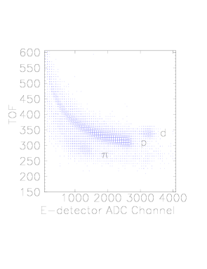
FIG. 2.: Raw ejectile time of flight (ADC channels) vs. energy deposited in the E detector by pions, protons and deuterons. Triggers from two charged particles tracks and (no K) were a prerequisite. This spectrum was used for identification of protons and pions.

All detectors are segmented because the energies of the coincident reaction particles need to be measured independently. Monte Carlo calculations suggest that eight $\Delta\phi$ segments are sufficient because of the tendency of the ejectiles to have significantly different azimuthal angles. The K detector was needed to obtain the necessary stopping power for the more energetic pions and protons. Identification of the charged particles was usually accomplished by their time of flight vs. energy correlation, where the start signal was supplied by the F detector and the stop signal was provided by the E detector. The pion and proton distributions were generally well separated. Fig. 2 shows a typical particle ID spectrum for accepted $p\pi^{+}$ coincidence events.

The more energetic ejectiles stop in the K detector, and superior particle identification is obtained by comparing the energies deposited in the K vs. the E detectors, as seen in Fig. 3.

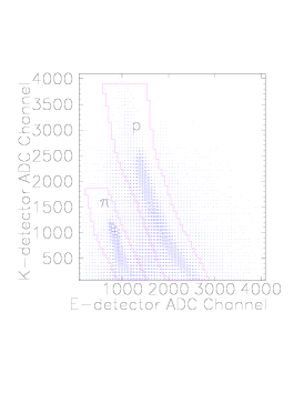
FIG. 3.: Particle identification cuts at 375 MeV for energetic ejectiles based on energy deposited in the K detector as function of energy loss in the E detector. Acceptable events had to be inside the regions outlined.

We measured the polarization observables $A_{ij}$ in two different ways:

1) by measuring the pions directly, in coincidence with protons (p+$\pi$ method), and

2) by reconstructing pion momenta from the measured proton and neutron momenta (p+n method).

The first method had the advantage of simplicity and high count rate, but we cannot measure pions at large angles due to the limited detector size. Therefore the spin dependent cross section ratios could be compared with theoretical spin correlation coefficients only at forward angles. The second method is free from this limitation, but at the cost of the low neutron detection efficiency and therefore much lower statistics.

B Measurement of p + $\pi^{+}$ coincidences

We accept events with two charged reaction particles (p and $\pi^{+}$) in coincidence. They must show separate tracks in the wire chambers WC1, WC2, trigger separate sections of the E detectors, and at least one section of the F detector, but not the veto scintillator (V). The trajectories of the protons and pions are deduced from the wire chamber position readings. Their angular resolution was limited primarily by multiple scattering in the 1.5 mm thick F detector and in the 0.18 mm thick stainless steel exit foil. Approximate angular resolutions (in the lab system) are $\sigma=0.5^{\circ}$ for protons and $1.0^{\circ}$ for pions. This resolution was fully sufficient for the angular variations expected.

The good intrinsic angular resolution of the wire chambers was used to check the consistency of the pion and neutron position readouts by tracing elastic protons to the hodoscope bars and comparing predicted and observed position readings. It was found that from run to run the beam axis and the detector symmetry axis could differ slightly in direction and also in their relative x and y coordinates at z=0 (the target center). We could also cross check the nominal z separation of the wire chambers since the separation and location of the hodoscope bars was fixed and well known. Small corrections of 1-3 mm had to be applied in software to the detector positions. After such corrections the remaining systematic angular error of the measured polar angles is about $0.04^{\circ}$.

Charged particles that do not stop in or before the K detector trigger the V detector and are tagged as likely elastic events and generally vetoed. At 400 MeV we reach the design limit of the charged particle detectors and the veto detector begins to see (and reject) the most energetic pions at small angles. In deducing the energy spectra account was taken of the differing non-linearity of light production for protons and pions by the plastic scintillators, as well as of energy losses in the exit foil, the F detector, air and other materials between the scintillators. After calibrations of all detector segments the detector stack provided an energy resolution for typical reaction protons and pions of about $\Delta E/E=.09$ (FWHM).

The missing mass spectra contain a background continuum (see Fig. 4), which at higher beam energies stretches slightly beyond the missing mass peak.

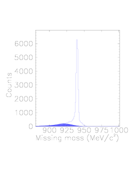
FIG. 4.: Neutron missing mass reconstructed from measured pion and proton momenta. The background spectrum shown (dark area) results if the atomic hydrogen in the target cell is replaced by Nitrogen gas.

The trajectory traceback indicates that this background is primarily caused by beam halo hitting the Al and teflon components of the target cell. Without target gas (and the beam heating normally produced by it) almost no background is seen. In order to obtain a realistic background shape near and below the missing mass peak the target cell was filled with $N_{2}$. This gas will produce some background of its own, but just as importantly it heats the circulating beam (as the Hydrogen gas would) and reproduces the ordinary beam halo. We found that the “$N_{2}$ spectra” seen after the common software cuts looked identical to the background “tail” in the Hydrogen missing mass spectra. Therefore, $N_{2}$ spectra were measured with good statistics, and their shape was later used to correct for background under the missing mass peak. Our statistically most accurate measurements were obtained in the p+$\pi$ mode, i.e., by observing pions and protons in coincidence.

C Measurement of p+n coincidences

Reaction neutrons in coincidence with protons were detected in a large hodoscope consisting of 16 long plastic scintillator bars. The bars were placed symmetrically about the beam direction in a plane defined by z=1.48 m. They were 15 cm deep and mounted so that their dimension in the y and x directions were 120 cm and 5 cm, respectively (see Fig. 1). The position in the y direction was determined from the differing arrival times of the scintillator light pulses read out by the top and bottom photomultipliers. The y-position resolution was $\sigma\approx 1.7$ cm. At 325 MeV the geometric acceptance for p + n detection is comparable to that for the $pp\rightarrow pp\pi^{0}\,$  branch; however, the achievable event detection rate is much smaller because of the low neutron detection efficiency. The neutron pulse height threshold was set as low as practical and corresponds to 5 MeV electrons for all bars. At this threshold a 15 cm thick plastic scintillator averages a neutron detection efficiency of about 0.17 for the neutron energies of this experiment [27].

A thicker neutron detector would be more efficient, but along with technical problems it would produce a correspondingly poorer time of flight resolution, since the length of the available flight path was limited to 1.5 m. In this experiment an additional reduction of the neutron detection efficiency arose because the E and K proton detectors are located in front of the neutron hodoscope and represent a 26 cm thick (polystyrene) absorber for the reaction neutrons. Resulting neutron losses in this “absorber” range from 30% for the highest energy neutrons to about 90% for those at the very lowest energies. As a consequence the energy averaged effective neutron detection efficiency was reduced to a value of about 0.07. Since neutron energies are measured and neutron reaction cross sections are known [28], corrections for energy dependent efficiency losses can and have been made, but the loss in counting rate seriously limited the statistics obtained.

The neutron energy was measured by neutron time of flight. In applying this method we use the correlated proton trigger from $\vec{p}\vec{p}\rightarrow pn\pi^{+}$ in the F detector. Since the proton arrival at the F detector is delayed one has to use a two-step process: First, the trigger time difference (F detector time minus hodoscope mean time) is measured. Next the timing must be corrected for the proton flight time to the F detector, since the F detector is triggered by the proton after it has traveled about 30 cm before reaching the F detector. This correction is based on the measured proton energy and reconstructed track length. Neutron flight times (TOF) range from 5 to 12 ns.

The dominant contribution to the TOF resolution comes from the 15 cm bar thickness, which constitutes 10% of the flight path and cannot be overcome with the available detectors. Smaller contributions come from the intrinsic timing resolution of the hodoscope (0.4 ns FWHM) and the F detector (0.5 ns FWHM, after amplitude walk correction). We note that the raw time resolution of the F detector is worse than the figure quoted above because of trigger walk in the electronics and because of the light loss and travel delay of light from parts of the large four-section F detector more distant from the photomultipliers. A substantial improvement was achieved by employing a pulse height compensation function. Overall, we see a neutron time of flight resolution with $\Delta T/T\approx 0.1$. Therefore, the missing mass (MM) peak for $\pi^{+}$ from p+n detection is not as sharp as for the corresponding neutron missing mass derived from p+$\pi^{+}$ events.

III Analysis

A Monte Carlo Simulations

Our Monte Carlo (MC) simulations of the experiment used the event generator GENBOD of the CERN library. The simulation was used to determine various limiting effects of the apparatus and to derive corresponding corrections. The code contained the detailed geometry of the detector systems and the density distribution of the gas target. In the MC simulation we took into account the loss of energy of the charged particles before entering the detectors, detector resolutions, charged particle multiple scattering, pion decay in flight, energy-dependent neutron detection efficiency and the probability of nuclear reactions of the reaction neutrons in the E and K detectors. In the MC simulation we have used a $pn$ final-state interaction (FSI) based on the Watson-Migdal theory, and the equations were derived following Morton [29]. We found that at the lower energies the FSI has a large effect on the overall coincidence acceptance. The simulation also provided a guide to the expected energy and angular distribution of the reaction products.

Pion counting losses caused by the limited detector depth are not large enough to be detectable in the shape of spectra; however, the Monte Carlo simulation shows that they must be considered. At 400 MeV the loss for pions is 14% because this fraction of the forward pions is too energetic to stop in the K detector. Only about 0.2% of the reaction protons penetrate past the K scintillators and are vetoed. The loss of high energy pions at small lab angles may create a small distortion of the 400 MeV p+$\pi$ data. Corrections to the 400 MeV spectra were not made since they would have to be very model dependent. We note parenthetically that the 400 MeV data from p+n coincidences do not have this systematic error, but within statistics they agree with overlapping $p+\pi^{+}$ results. No “veto” losses are seen at 375 MeV or below.

The finite size of the individual detector segments produces some counting losses since two sections have to trigger for acceptable events. However, systematic effects for the polarization observables are unlikely since the protons have no strong $\phi$ correlations with the pions. The segmentation used leads to a loss of about 7% in counting statistics for the p+$\pi^{+}$ branch. There is no such loss for p+n detection. The charged particle detectors cover polar angles between $5^{\circ}$ and $40^{\circ}$ in the laboratory frame. Hence a large number of pions miss the detector. The total $p+\pi^{+}$ coincidence acceptance ranges from 21% at 325 MeV to 15% at 400 MeV.

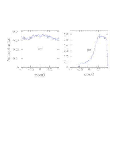
FIG. 5.: Monte Carlo simulation for (a) the p+n and (b) the p+$\pi^{+}$ acceptance, in the center of mass system. The partial acceptance for pions seen in the $p\pi$ diagram at $\theta_{\pi}\geq 70^{\circ}$ results from the dominating forward boost for low energy pions. The cutoff at $cos~{}\theta_{\pi}\approx-0.5$ is caused by detector thresholds for the lowest ejectile energies.

For p+n detection the MC simulation shows that the acceptance is symmetric about $90^{\circ}$ although not quite isotropic. (See Fig. 5a.) Acceptance losses for p+n coincidences attributable to the detector geometry alone are of the order of 25%. The major cause is the central hole in the proton detectors. After all geometric acceptance losses and detector inefficiencies for neutron detection are taken into account the computed overall detection efficiency for pn coincidence events is 3.5%. It is seen in Fig. 5a that the angular variations of the coincidence efficiency for the reconstructed pion are small. This is so despite the fact that we cannot detect protons at angles $\leq 5^{\circ}$ and neutrons at angles $\leq 2.5^{\circ}$ and have reduced coverage by the hodoscope of some azimuthal angles for large neutron polar angles. The Monte Carlo acceptance curves for p+n detection suggest that within the statistical accuracy of the experiment the spin-correlation parameters integrated over $\rm\theta_{\pi}$ and $\rm\phi_{\pi}$ would need no significant correction. Fig. 5b shows the Monte Carlo simulation for $p\pi^{+}$ acceptance as a function of $cos~{}\theta_{\pi}$. For $p\pi^{+}$ coincidences the apparatus acceptance is only useful for $\theta_{\pi}\leq 70^{\circ}$. Therefore, the integrated spin correlation coefficients will be deduced from the combined sets of the $p+\pi^{+}$ and p+n coincidences.

B Analysis of p+$\pi^{+}$ coincidences

The energies of the charged particles are measured by the plastic scintillator systems E and K. The calculated momenta of the unobserved particles strongly depend on the energies of the detected ejectiles, so considerable attention was given to a careful energy calibration of all detectors. The complex geometry of the segmented plastic detectors required corrections for light collection that primarily were derived from the observation of elastically scattered protons. An xy-position correction factor was applied to account for this dependence. A second pulse height correction factor was applied to compensate for a variation of phototube gains with the orientation of the magnetic guide field for the target polarization. For details see [22].

The corrected pulse heights L were converted into the deposited energy E using

$$E=L+k_{1}\sqrt{L}+k_{0}$$ (1)

The nonlinear term corrects for light quenching in plastic scintillators. $k_{0}$ and $k_{1}$ are calibration constants. L is the sum of the light pulse from the E and the K detectors in MeV and is given by $L=c_{1}(E_{light}+c_{2}K_{light}+c_{3})$. The constants $c_{1},c_{2},c_{3}$ are gain matching constants, and $E_{light}$ and $K_{light}$ correspond to the observed light pulses in the $E$ and the $K$ detectors respectively. The constant $c_{3}$ corrects for small energy losses in the material between the E and K detectors. It is small and set equal to zero when there is no K trigger.

The total kinetic energy of the charged particle was calculated by also taking account of the energy lost by the charged particle on its way to the E-detector. The calibration constants were fine tuned by utilizing kinematical relations. We required that the missing mass centroid was at its predicted value and that the angular distribution of the pions from the simultaneous measurement of the reaction $\vec{p}\vec{p}\rightarrow pp\pi^{0}$ was symmetric in the c.m. system about $\theta_{\pi}=90^{0}$. This symmetry was sensitive to the relative size of the calibration coefficients. However, the variation of the deduced spin correlation coefficients under different reasonable combinations of the calibration constants was small and less than the statistical errors.

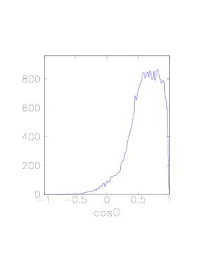
FIG. 6.: Detected pions at 325 MeV as a function of $\theta_{\pi}$. Only events with $cos\,\theta_{\pi}\geq 0.4$ were used for the analysis.

Fig. 6 shows the directly observed $\pi^{+}$ differential cross sections plotted against $cos\,\theta_{\pi}$ in the c.m. coordinate system. We note that there are almost no counts for pion back angles $-1<cos\,\theta_{\pi}<0$ , as expected from the apparatus acceptance (compare Fig. 5b).

FIG. 7.: Distributions of the calculated missing mass $\rm m_{x}$ for $p+\pi^{+}$ detection at 325 MeV bombarding energy, for the four combinations of vertical beam and target polarization. A sharp peak ($\approx\rm 3.5~{}MeV/c^{2}$ FWHM) is seen at 939.6 $\rm MeV/c^{2}$, the neutron rest mass. The shaded region indicates the background distribution.

Fig. 7 shows missing mass spectra seen at 325 MeV for four combinations of vertical beam and target polarization at equal integrated luminosity. The polarization observables are obtained from the ratio of “yields” for different spin orientations. The yields to be used are the integrated counts inside the missing mass gates minus background. In order to estimate the error from uncertainties in the background we varied the background subtraction by $\pm$25%. The effect on the final results was smaller than the statistical error. At 325 MeV the off-line resolution of the neutron missing mass peak was $\rm\sigma=1.4~{}MeV/c^{2}$. Even before software cuts and background correction it is apparent from Fig. 7 that different spin combinations produce very different yields.

It turns out that the decay in flight of pions plays a negligible role for these data. It will appreciably affect only the (undetected) backward scattered pions as these have much lower lab energies than the forward pions. For the final analysis we selected the $pp\rightarrow pn\pi^{+}\,$events of interest by using a gate of 30 MeV or wider over the relevant missing mass peak. Gates as narrow as 10 MeV did not produce systematic changes, neither did they measurably reduce background induced errors. However, the narrower gates lead to some loss of statistics.

C Analysis of p+n coincidences

This detection channel has the advantage that the acceptance for the detection of p+n coincidences has little angular variation. So $\theta_{\pi}$ and $\phi$-dependent acceptance corrections generally can be ignored. Therefore the p+n coincidences importantly complement the p+$\pi^{+}$ channel. Reliance on the p+n angular distributions at large angles leads to larger statistical error bars relative to p+$\pi^{+}$ (forward) region. However, the combination of the two detection modes provides data for the full angular range and so keeps the integrated spin correlation coefficients model independent.

In the p+n analysis we first analyzed only those events where all three reaction particles ($p,n$ and $\pi^{+}$) were detected (the triple coincidence). Next we evaluated the case where the pions missed the E detector, but a proton and a neutron were detected (double coincidence). The energy of reaction protons was determined using the calibration constants described above. The energy of the neutrons was determined by measuring their time of flight (TOF) to the hodoscope. The MC simulation showed that although F was always triggered by protons for a p+n double coincidence, in the case of a $pn\pi^{+}$ triple coincidence it was triggered by the faster pions. Therefore, depending on the event class, we corrected the neutron TOF by adding the time it takes either for the coincident proton or the pion to reach the F detector. A calculated offset was added to the timing signal of each hodoscope bar in order to make the timing information independent of the bar electronics. This correction was obtained by calibrating the timing circuits with elastic proton scattering.

For $\theta_{\pi,lab}\leq 40^{\circ}$ we observe $pn\pi^{+}$ triple coincidences, which are practically free of background. (The absence of accepted events from the $N_{2}$ gas target showed that the triple $pn{\pi^{+}}$ hardware coincidence under standard software conditions eliminates all background from the target wall and target impurities.) These events proved very valuable in assessing the correct shape of the missing mass peaks in p+n and p+$\pi$ events. If a missing mass spectrum for triple coincidences is calculated based on the pion and proton momenta the (neutron) missing mass spectrum shows a very sharp peak as in Fig. 4, but there is no “background tail” at all. The triple coincidence spectrum confirms the background subtraction shown in Figs. 4 and 7.

If the same triple coincidence events are used to calculate the (pion) missing mass by using the proton and neutron momenta (i.e., ignoring the simultaneously known pion momenta) we obtain the spectrum shown in Fig. 8. This spectrum can be used as a standard for the missing mass that p+n (double coincidence) events would have in the absence of background.

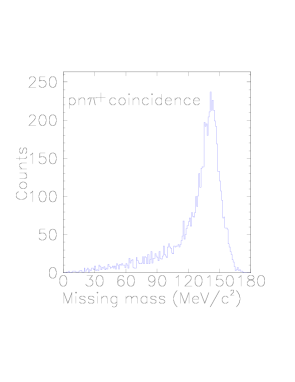
FIG. 8.: Missing mass spectrum for $pn\pi^{+}$ triple coincidences, based on the measured neutron and proton energies. This spectrum contains no background from any competing reaction. The missing mass tail here is a consequence of some inaccurately measured neutron momenta. See text.

The MM distribution peaks at the true pion mass of 139.6 MeV, but there also is a “tail” over a wide range of the missing mass spectrum, which is not background related. We conclude that the counts in the MM tail of Fig. 8 represent genuine $pn\pi^{+}$ events from the Hydrogen target, albeit events with poorly determined neutron momenta. We estimate that up to 20% of the p+n coincidences contain neutron observables that are distorted by interactions of neutrons with the K or E detectors. E.g., neutrons can undergo small angle elastic and inelastic scattering, but still reach the hodoscope. This would lead to incorrect readings for polar and azimuthal neutron angles and hence to an incorrect missing mass calculation.

Such events with poorly determined missing masses were excluded from further analysis. For all p+n events we reduce genuine background and avoid analyzing measurably distorted p+n events by using a missing mass gate from 100 to 160 MeV.

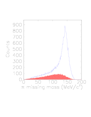
FIG. 9.: The $\pi^{+}$ missing mass ($m_{x}$) spectrum at 375 MeV calculated from the measured neutron and proton momenta. The deduced background is shown by the lower distribution. For the analysis events with $100\leq m_{x}\leq 160$ were accepted.

Using the triple coincidence MM spectrum as a standard, the background under the missing mass peak for two-particle p+n coincidences was deduced by adding a fraction of the measured unstructured $N_{2}$ background continuum to the “standard” MM spectrum until the observed p+n MM spectrum shape was reproduced. The tail in the latter is flatter and more pronounced because of actual background contributions. To estimate the error in this procedure we varied the match until it became unrealistic ($\pm 15\%$). A typical missing mass spectrum for p+n (double coincidence) detection is shown in Fig. 9. In the final result the uncertainty from this background subtraction was about half as large as the statistical error.

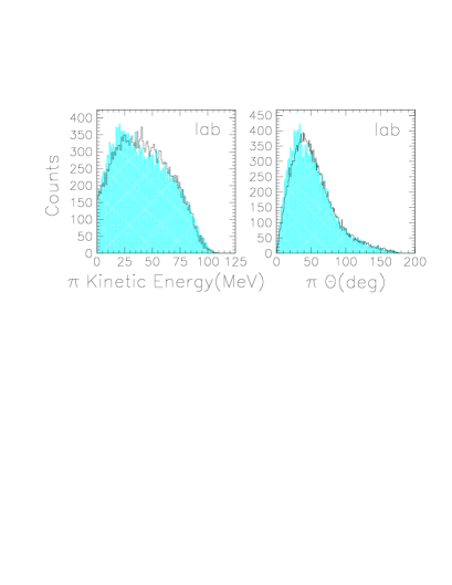
FIG. 10.: Energy and angular distributions for p+n coincidences at 375 MeV, compared with Monte Carlo projections (solid lines) in the laboratory system. Agreement is expected for the kinematic limits. However, the distributions may differ because the $l_{\pi}=0$ assumption for the MC simulation is an oversimplification at and above 325 MeV.

At 375 MeV the resolution of the pion MM peak was $\rm\sigma=9~{}MeV/c^{2}$. Pion angular and energy distributions from p+n detection were computed using only events inside this missing mass gate. Some resulting distributions are compared with Monte Carlo projections for the laboratory coordinate system in Fig. 10.

The end points of these distributions agree well with the kinematics of the experiment as they must. The solid curves represent pure $\l_{\pi}=0$ MC calculations. Although $\l_{\pi}=0$ makes the major contribution, this MC assumption produces oversimplified energy and angular distributions. Nevertheless, the simulated distributions agree reasonably well with the data.

Fig. 11 shows the deduced pion angular distribution in the center of mass system. The reconstructed $\pi^{+}$ distribution is plotted against $cos\,\theta_{\pi}$ in the center of mass (corrected for background and for the slightly non-uniform acceptance shown in Fig. 5a). As expected, it is non-isotropic and symmetric about $\theta_{\pi}=90^{o}$ within statistical errors.

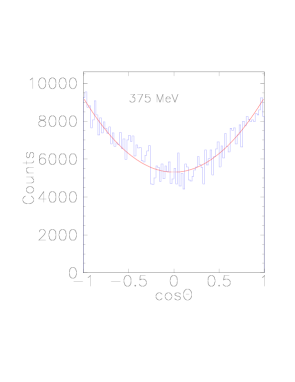
FIG. 11.: The relative $\pi^{+}$ production cross section $\sigma_{0}(cos~{}\theta_{\pi})$ at 375 MeV as deduced from p+n coincidences.

IV Polarization Observables

A Formalism for spin correlation coefficients

The meaning of the symbols $A_{ij}$ used for polarization observables is defined by Eq. 2. In terms of the “Cartesian polarization observables” the spin–dependent cross section is written as

$$\sigma(\xi,\vec{P},\vec{Q})\ =\ \sigma_{0}(\xi)\cdot\left[1+\sum_{i}P_{i}A_{i0}(\xi)+\sum_{j}Q_{j}A_{0j}(\xi)+\sum_{i,j}P_{i}Q_{j}A_{ij}(\xi)\right]\ ,$$ (2)

where $\xi$ stands for the pion coordinates $\rm\theta_{\pi},\varphi_{\pi}$, the energy defining pion momentum $p_{\pi}$, and the proton coordinates $\rm\theta_{p}$ and $\rm\varphi_{p}$. The unpolarized cross section is $\sigma_{0}(\xi)$, and the polarization of the beam and the target is denoted by the vectors $\vec{P}=(P_{x},P_{y},P_{z})$ and $\vec{Q}=(Q_{x},Q_{y},Q_{z})$. The subscripts $i$ and $j$ stand for $x$, $y$ or $z$ and the sums extend over all possibilities. The resulting 15 polarization observables include the beam analyzing powers A_i0, the target analyzing powers A_0j and the spin correlation coefficients A_ij.

The partial wave analysis for $\vec{p}\vec{p}\rightarrow pn\pi^{+}$ is similar to that for $\vec{p}\vec{p}\rightarrow pp\pi^{0}$ in terms of transition amplitudes. However, the $pp\rightarrow pn\pi^{+}\,$ transitions have isoscaler as well as isovector components. The different isospins in $\vec{p}\vec{p}\rightarrow pn\pi^{+}$ modify the selection rules for the reaction and lead to polarization observables that are different. The general relations between reaction amplitudes and angular distributions, however, remain almost identical. The applicable partial wave formalism has been discussed in detail in [26]. We use the same notation as in [26] and reiterate some relevant definitions and theoretical relations below. Several names are in use for polarization observables. Their meaning is as defined below:

$$A_{\Sigma}(\xi)\ \equiv\ A_{xx}(\xi)+A_{yy}(\xi)\$$ (4)

$$A_{\Delta}(\xi)\ \equiv\ A_{xx}(\xi)-A_{yy}(\xi)\$$ (5)

$$A_{\Xi}(\xi)\ \equiv\ A_{xy}(\xi)-A_{yx}(\xi)\$$ (6)

For identical particles in the entrance channel there are seven independent polarization observables:

$$A_{y0}(\xi),\ A_{\Sigma}(\xi),\ A_{zz}(\xi),\ A_{xz}(\xi),\ A_{\Delta}(\xi),\ A_{\Xi}(\xi)\ ,\ A_{z0}(\xi).$$ (7)

This paper addresses the first five observables of this set. The remaining two, $A_{\Xi}(\xi)$ and $A_{z0}(\xi)$, can be non-zero only for non-coplanar final states. In the following we will integrate over the angles of the nucleon, and thus these two observables vanish if parity is conserved.

It is common to display the bombarding energy dependence of the observables in terms of the dimensionless parameter eta (${\eta}$), which is defined as

$$\eta\ =\ p_{\pi,max}/m_{\pi^{+}}\ ,$$ (8)

The term “near threshold” is meant to include the energy region with $\eta<1$, i.e., below 400 MeV. Setting $c=\hbar=1$, the maximum value of the $\pi^{+}$ momentum is found from:

$$p_{\pi,max}\ =\ \frac{1}{2\sqrt{s}}\sqrt{[s-(m_{n}+m_{p}+m_{\pi^{+}})^{2}][s-(m_{n}+m_{p}-m_{\pi^{+}})^{2})]}\ ,$$ (9)

where $\sqrt{s}$ is the total center-of-mass energy, and $m_{p}$, $m_{n}$, and $m_{\pi^{+}}$ are the masses of the proton, the neutron, and the pion, respectively. (We explicitly labeled the pion as $\pi^{+}$ to emphasize that the $\pi^{+}$ and $\pi^{0}$ mass difference matters here.)

Below we quote some useful relations between integrated spin correlation coefficients and some directly observable spin dependent cross sections. For two colliding spin 1/2 particles, one can define three total cross sections, two of which depend on the spin. The total cross sections are related to the observables above by

$$\sigma_{tot} = \int\sigma_{0}(\xi)d\Omega_{p}d\Omega_{\pi}dp_{\pi}$$ (11)

$$\Delta\sigma_{T} = -\int\sigma_{0}(\xi)A_{\Sigma}(\xi)d\Omega_{p}d\Omega_{\pi}dp_{\pi}$$ (12)

$$\Delta\sigma_{L}\ = -2\int\sigma_{0}(\xi)A_{zz}(\xi)d\Omega_{p}d\Omega_{\pi}dp_{\pi}$$ (13)

Here $d\Omega=d\cos\theta\,d\varphi$, and the integration extends over $0\leq\theta\leq\pi$, and all pion momenta. $\Delta\sigma_{L}/\sigma_{tot}$ and $\Delta\sigma_{T}/\sigma_{tot}$ can have values between $-2$ and +2.

The integrated spin correlation coefficients are defined as:

$$\overline{A_{\Sigma}} = [\int\sigma_{0}(\xi)A_{\Sigma}(\xi)d\Omega_{p}d\Omega_{\pi}dp_{\pi}]/\sigma_{tot}$$ (15)

$$\overline{A_{zz}} = [\int\sigma_{0}(\xi)A_{zz}(\xi)d\Omega_{p}d\Omega_{\pi}dp_{\pi}]/\sigma_{tot}$$ (16)

$$\overline{A_{\Delta}} = [\int\sigma_{0}(\theta_{\pi})A_{\Delta}(\theta_{\pi})sin\theta_{\pi}d\theta_{\pi}]/\sigma_{tot}$$ (17)

$$\overline{A_{xz}} = [\int\sigma_{0}(\theta_{\pi})A_{xz}(\theta_{\pi})sin\theta_{\pi}d\theta_{\pi}]/\sigma_{tot}$$ (18)

$$\overline{A_{y0}} = [\int\sigma_{0}(\theta_{\pi})A_{y0}(\theta_{\pi})sin\theta_{\pi}d\theta_{\pi}]/\sigma_{tot}$$ (19)

We note that $\overline{A_{\Sigma}}$ and $\overline{A_{\Delta}}$ differ by a scale factor from $\Delta\sigma_{T}$ and $\Delta\sigma_{L}$. These quantities in principle can be measured directly, although in this study they are derived from integration over $A_{\Sigma}(cos\theta_{\pi})$ and $A_{zz}(cos\theta_{\pi})$. The remaining three integrals must be defined differently. Here the spin correlations $A_{ij}$ are taken at $\phi_{\pi}=0$. (They cannot be integrated over the variable $\phi_{\pi}$ since they would vanish, as will be seen below).

Based on the dominance of Ss, Sp, Ps, and Pp transitions, general symmetries and spin coupling rules [26], the cross sections and spin correlation coefficients must have the general form:

$$\sigma_{0}(\xi) = a_{00}+b_{00}\mbox{$(3\cos^{2}\theta_{\pi}-1)$}+c_{0}(3\cos^{2}\theta_{p}-1)$$ (23)

$$+d_{0}\mbox{$(3\cos^{2}\theta_{\pi}-1)$}(3\cos^{2}\theta_{p}-1)+e_{0}\sin 2\theta_{p}\sin 2\theta_{\pi}\cos\Delta\varphi$$

$$+f_{0}\sin^{2}\theta_{p}\sin^{2}\theta_{\pi}\cos 2\Delta\varphi$$

$$\sigma_{0}(\xi)A_{y0}(\xi) = [{\{a_{y0}+b_{y0}(3\cos^{2}\theta_{p}-1)\ \}\sin\theta_{\pi}+\{c_{y0}+d_{y0}}(3\cos^{2}\theta_{p}-1)\}\sin 2\theta_{\pi}]\cos\varphi_{\pi}$$ (27)

$$+[e_{y0}+f_{y0}\cos\theta_{\pi}+g_{y0}\mbox{$(3\cos^{2}\theta_{\pi}-1)$}]\sin 2\theta_{p}\cos\varphi_{p}$$

$$+[h_{y0}\sin\theta_{\pi}+i_{y0}\sin 2\theta_{\pi}]\sin^{2}\theta_{p}\cos(2\varphi_{p}-\varphi_{\pi})$$

$$+j_{y0}\sin 2\theta_{p}\sin^{2}\theta_{\pi}\cos(2\varphi_{\pi}-\varphi_{p})$$

$$\sigma_{0}(\xi)A_{\Sigma}(\xi) = a_{\Sigma}+b_{\Sigma}\mbox{$(3\cos^{2}\theta_{\pi}-1)$}+c_{\Sigma}(3\cos^{2}\theta_{p}-1)$$ (30)

$$+d_{\Sigma}(3\cos^{2}\theta_{p}-1)\mbox{$(3\cos^{2}\theta_{\pi}-1)$}+e_{\Sigma}\sin 2\theta_{p}\sin 2\theta_{\pi}\cos\Delta\varphi$$

$$+f_{\Sigma}\sin^{2}\theta_{p}\sin^{2}\theta_{\pi}\cos 2\Delta\varphi$$

$$\sigma_{0}(\xi)A_{zz}(\xi) = a_{zz}+b_{zz}\mbox{$(3\cos^{2}\theta_{\pi}-1)$}+c_{zz}(3\cos^{2}\theta_{p}-1)$$ (33)

$$+d_{zz}(3\cos^{2}\theta_{p}-1)\mbox{$(3\cos^{2}\theta_{\pi}-1)$}+e_{zz}\sin 2\theta_{p}\sin 2\theta_{\pi}\cos\Delta\varphi$$

$$+f_{zz}\sin^{2}\theta_{p}\sin^{2}\theta_{\pi}\cos 2\Delta\varphi$$

$$\sigma_{0}(\xi)A_{\Delta}(\xi) = [a_{\Delta}+b_{\Delta}(3\cos^{2}\theta_{p}-1)]\sin^{2}\theta_{\pi}\cos 2\varphi_{\pi}$$ (36)

$$[c_{\Delta}+d_{\Delta}\mbox{$(3\cos^{2}\theta_{\pi}-1)$}]\sin^{2}\theta_{p}\cos 2\varphi_{p}$$

$$e_{\Delta}\sin 2\theta_{p}\sin 2\theta_{\pi}\cos(\varphi_{p}+\varphi_{\pi})$$

$$\sigma_{0}(\xi)A_{xz}(\xi) = [\{a_{xz}+b_{xz}(3\cos^{2}\theta_{p}-1)\}\sin\theta_{\pi}+\{c_{xz}+d_{xz}(3\cos^{2}\theta_{p}-1)\}\sin 2\theta_{\pi}]\cos\varphi_{\pi}$$ (40)

$$+[e_{xz}+f_{xz}\cos\theta_{\pi}+g_{xz}\mbox{$(3\cos^{2}\theta_{\pi}-1)$}]\sin 2\theta_{p}\cos\varphi_{p}$$

$$+[h_{xz}\sin\theta_{\pi}+i_{xz}\sin 2\theta_{\pi}]\sin^{2}\theta_{p}\cos(2\varphi_{p}-\varphi_{\pi})$$

$$+j_{xz}\sin 2\theta_{p}\sin^{2}\theta_{\pi}\cos(2\varphi_{\pi}-\varphi_{p})$$

Here we have used the abbreviation $\Delta\varphi\equiv\varphi_{p}-\varphi_{\pi}$. The Eqs. IV A explicitly depend on the four angles $\theta_{p}$, $\varphi_{p}$, $\theta_{\pi}$ and $\varphi_{\pi}$. The energy dependent parameter $p_{\pi}$ is contained in the coefficients. Statistics in this experiment are not sufficient to present double or higher differential cross sections. Therefore, we integrate over the angles of the proton and use energy and momentum conservation to eliminate all angles except $\theta_{\pi}$ and $\phi_{\pi}$. This leads to a set of much simpler equations:

$$\sigma_{0}(\zeta) = a_{00}+b_{00}\mbox{$(3\cos^{2}\theta_{\pi}-1)$}$$ (42)

$$\sigma_{0}(\zeta)A_{y0}(\zeta) = [{a_{y0}}\sin\theta_{\pi}+{c_{y0}}\sin 2\theta_{\pi}]\cos\varphi_{\pi}$$ (43)

$$\sigma_{0}(\zeta)A_{\Sigma}(\zeta) = a_{\Sigma}+{b_{\Sigma}}\mbox{$(3\cos^{2}\theta_{\pi}-1)$}$$ (44)

$$\sigma_{0}(\zeta)A_{zz}(\zeta) = a_{zz}+{b_{zz}}\mbox{$(3\cos^{2}\theta_{\pi}-1)$}$$ (45)

$$\sigma_{0}(\zeta)A_{\Delta}(\zeta) = {a_{\Delta}}\sin^{2}\theta_{\pi}\cos 2\varphi_{\pi}$$ (46)

$$\sigma_{0}(\zeta)A_{xz}(\zeta) = [{{a_{xz}}\sin\theta_{\pi}+{c_{xz}}}\sin 2\theta_{\pi}]\cos\varphi_{\pi}$$ (47)

The symbol $\zeta$ now represents the reduced set of variables {$p_{\pi},\theta_{\pi},\phi_{\pi}$}. These equations display a simple and characteristic $\phi_{\pi}$ dependence of the different polarization observables and show the expected $\theta_{\pi}$ dependence. The coefficients $a_{\nu},b_{\nu},\ldots$ for the set IV A correspond to those in Eqs.  IV A. They are obtained by one- or two-parameter fits to the observed angular distributions, separately for each observable.

B Extraction of polarization observables

The data analysis, as described in the previous sections, identifies the reaction particles, assesses the background for each spectrum and calculates the kinematic variables and spin dependent cross sections of the reaction products. It produces event files which contain kinematically complete information for all detected reaction particles. For each beam energy there are 12 such event files, one for each combination of beam and target spin. These yields are first corrected for the beam luminosity, which can vary for beam “spin up” and “spin down” subcycles, and for the background measurement. The background correction was made for each selected $\theta_{\pi}$ angle bin individually. The ratios $R_{i}$ of yields for different spin combinations, integrated over a chosen $\theta_{\pi}$ range, are then analyzed as a function of $\phi_{\pi}$, because the allowed $\phi_{\pi}$ dependence can be predicted from spin coupling rules [21]. For this energy range, only final states with pn or pion angular momentum of 0 and 1 are expected to be significant. In a previous measurement of $pp\rightarrow d\pi^{+}$ at 400 MeV it was found that any $l_{\pi}=2$ contribution is very small [30]. This allows us to consider only transitions to Ss, Sp, Ps and Pp final states in the analysis. Sd and Ds transitions would affect the energy dependence of the coefficients only and so are very difficult to separate from Pp transitions [26]. They will be ignored in this analysis. We then have explicit predictions for the expected $\theta$ and $\phi$ dependences from eq. IV A.

The combination of p+$\pi^{+}$ and p+n measurements provides model-independent values for the polarization observables for all polar and azimuthal angles of the pion. The low neutron detection efficiency and the resulting low statistical accuracy of the p+n data make it advisable to display the combined data using some theoretical guidance. As shown below, $A_{\Sigma}(\theta_{\pi}),A_{\Delta}(\theta_{\pi})$, and $A_{zz}(\theta_{\pi})$ must be symmetric about $\theta_{\pi}=90^{\circ}$ for the transitions considered. So a good analysis in terms of the pion coordinates does not require the (redundant) data at large polar angles. This simplification and the fact that all published theoretical predictions have been presented in terms of the pion coordinates makes these coordinates our preferred system for the analysis.

The microscopic relations between the coefficients and the transition amplitudes can be derived from the partial-wave expansion described in the appendix of [26], but they are complicated. Moreover, the number of individual $pp\rightarrow pn\pi^{+}\,$amplitudes contributing above 350 MeV has become too large (19 rather than the 12 for $pp\rightarrow pp\pi^{0}\,$), since isospin 1 and 0 are present in the final state. They could not be deduced individually from the $pp\rightarrow pn\pi^{+}\,$data available.

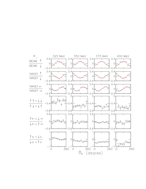
FIG. 12.: The yield related ratios $(R_{i}-1)/(R_{i}+1)$ as a function of the pion azimuthal angle $\phi_{\pi}$ for data integrated over all other coordinates. The specific beam and target spin combinations selected are listed on the left. For multiple arrows the orientation of the beam spin is shown first. Longitudinal polarization is indicated by the symbols o (opposite) and a (along beam direction). The solid curves represent a least-square fit using the expected theoretical $\rm\phi_{\pi}$ dependence.

When calculating the value of a polarization observable from Eqs. IV A or IV A, one evaluates the ratio $A_{ij}(\xi)=\sigma_{0}(\xi)A_{ij}(\xi)/\sigma_{0}(\xi)$, so the overall normalization of all terms in these equations cancels. As seen from Eqs. IV A the yield ratios $R_{i}(\phi_{\pi})$ could either be constant or have a $\phi_{\pi}$ or 2$\phi_{\pi}$ dependence. This is borne out by the data (compare Fig. 12).

The polarization observables were deduced by evaluating the observed $\phi_{\pi}$ dependences of the ratios $R_{i}$ for selected beam and target spin combinations. This evaluation is complex when longitudinal as well as transverse beam polarizations are present at the same time. Therefore, the devolution process uses the computerized fitting routine BMW [31], which was written for this purpose.

Fig. 12 shows the $\phi_{\pi}$ dependence of six spin dependent yield ratios. The data for the beam (first arrow) and target spin combinations indicated have been integrated over all coordinates other than the coordinate ${\phi}_{\pi}$. The curves are fits using one to three components of the Eqs. IV A. The first three rows present different ways to extract the analyzing power $A_{y}(\phi_{\pi})$. The lower three rows contain information on $A_{\Sigma}=A_{xx}+A_{yy}$, $A_{\Delta}=A_{xx}-A_{yy}$, and contributions from $A_{zz}$ and $A_{xz}$. For some ratios the statistics are marginal, and one cannot exclude the potential presence of $\,l$ components higher than included in the analysis, but the $\phi_{\pi}$ dependent fits show that the inclusion of Ss, Sp, Ps, and Pp transitions is sufficient to reproduce the data within experimental errors.

For the simultaneous detection of neutrons and protons, our data sample the full range for $\theta_{\pi}$, although with low statistics. We combine the p+$\pi$ and p+n data sets to obtain optimal spin correlation coefficients for the full angular region. We avoid difficulties generated by the non-uniform detector acceptances in $\theta_{\pi}$ by evaluating the p+n and $p+\pi$ relations $A_{ij}(cos~{}\theta_{\pi})$, which are ratios of cross sections at a given angle. (Our detection efficiency does not depend on spin, and the detector acceptances cancel out for $A_{ij}(cos~{}\theta_{\pi})$.) The combined p+n and p+$\pi^{+}$ sets yield complete angular distributions with their best statistics at forward angles. The unpolarized angular distribution $\sigma_{0}(\theta_{\pi})$ was obtained to sufficient accuracy from the p+n branch. The angular distributions can now be integrated. To best account for experimental errors we have chosen to integrate Eqs. IV A directly after the fitting coefficients are deduced.

Some of the polarization ratios measured are not independent, as the first three rows in Fig. 12 show. The reaction has additional redundancies. If parity is conserved and if we have identical particles in the entrance channel this redundancy can give us back-angle information for $A_{y}$ even though our detectors only cover forward polar angles for the direct detection of pions. The correlation we use repeatedly is

$$A_{ij}(\theta_{p},\phi_{p},\theta_{\pi},\phi_{\pi})\\ =A_{ji}(\pi-\theta_{p},\phi_{p}+\pi,\pi-\theta_{\pi},\phi_{\pi}+\pi)$$ (49)

This relation holds for $\rm i\neq j$ and also for i=j. E.g., since both $A_{xz}$ and $A_{zx}$ are measured at forward angles, we will obtain the back angle information for $A_{xz}$ from the $A_{zx}$ measurement at forward angles. The polarization observables $A_{xz}$ and $A_{zx}$ are not symmetric about $\theta_{\pi}=90^{\circ}$, so this redundancy becomes very useful.

V Results

A Polarization observables

It follows from Eq. 49 that the observables $A_{\Sigma}$, $A_{\Delta}$, and $A_{zz}$ are symmetric about $\theta_{\pi}=90^{\circ}$ ($cos\,\theta_{\pi}=0$). Within statistical errors the experimental data agree with this expectation. In Fig. 13 we have reduced the scatter from the low statistics of the p+n coincidences by combining the corresponding data for forward and back polar angles. The data for $cos\,\theta_{\pi}\geq 0.5$ are dominantly determined by events from $p+\pi$ coincidences. In agreement with theoretical expectations there is only a slow dependence on the polar angle, so the lack of good statistics near $\theta=90^{\circ}$ does not impede comparison with theory or the extraction of good values for the integrated polarization observables.

Fig. 14 shows results for $A_{y}(\theta_{\pi})$ and $A_{xz}(\theta_{\pi})$ for the full angular range so potential asymmetries can be seen. The statistically most accurate data were obtained for 375 MeV. Here and at 400 MeV the Jülich model is at odds with the data. The fit with Eq. IV A (solid lines) does much better. Still, a close inspection of the fits shows some small, but statistically significant differences between the partial wave curve and the data at very small and very large angles. We also see from Table I that the $\chi^{2}$ value for the $A_{y}$ fit has become large. The $A_{y}$ data suggest that higher partial waves enter at 375 MeV, but the experimental uncertainties discourage the extraction of relatively small contributions.

The fits obtained with Eq. IV A are good (i.e., $\chi^{2}\approx 1$ for all curves except for $A_{y}$ at 375 and 400 MeV). Therefore Eqs. IV A together with the coefficients of Table II can be used to represent the new data. The coefficients in these equations are bilinear sums of the reaction amplitudes. Their experimental values are given in Table II. This set is also used to obtain the integrated spin correlation coefficients. Integration of the angular distributions shown above produces the spin correlation coefficients in Cartesian coordinates. These coefficients were the original objective of this experiment. They are now known with good statistical accuracy and are given in Table III. A comparison of these integrated polarization observables as a function of beam energy with predictions of the Jülich model is shown in Fig. 15.

For completeness we note here that our attempt to extract non-coplanar angular distributions for $A_{z0}$ produced results (not shown) that were consistent with zero. This is different from the $pp\rightarrow pp\pi^{0}\,$results, but has no obvious explanation.

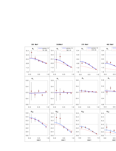
FIG. 13.: $\theta_{\pi}$ dependence for the polarization observables $A_{\Sigma}\equiv A_{xx}+A_{yy}$, $A_{\Delta}\equiv A_{xx}-A_{yy}$, and $A_{zz}$, in cartesian units. Data for the range $0.5<~{}cos~{}\theta~{}<1$ are primarily determined by the p+$\pi$ coincidences. The remaining points come from the p+n coincidences. The error bars include all random errors as well as estimated uncertainties from background subtraction. The dashed lines are Jülich model predictions by Hanhart et al.[22]. The solid lines show fits with the Eqs. IV A.

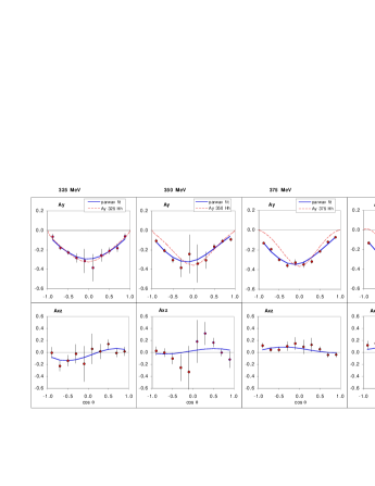
FIG. 14.: $\theta_{\pi}$ dependence for the polarization observables $A_{y}$ and $A_{xz}$ in cartesian units. The dashed lines are Jülich predictions. The solid lines show fits to the data using the Eqs. IV A.

It is clear from Figures 13, 14, and 15 that the distributions based on the Jülich model are in good agreement with the data at 325 MeV. However, above $\eta=0.7$ they produce ever larger $\chi^{2}$ values when compared to the data. These disagreements become striking for $A_{\Sigma}$ and $A_{y}$. The failures are most visible for $A_{y}$, an observable sensitive to admixtures of higher partial waves. (More serious disagreements with this model have been seen for the isovector production in $pp\rightarrow pp\pi^{0}\,$[26]. However, as discussed below, in this energy region isovector terms contribute less than 10% to the $pp\rightarrow pn\pi^{+}\,$cross section. The observed differences in $pp\rightarrow pn\pi^{+}\,$grow well beyond this level.)

Our partial wave analysis, which includes Ss, Sp, Ps, and Pp transitions, generally provides fits to the measured angular distributions with $\chi^{2}$ (per degree of freedom) values near 1. The exceptions are $A_{y}$ at 375 and at 400 MeV, where the cross sections are largest and the statistics are good. Some $\chi^{2}$ values as large as 3.9 are found if only statistical errors are considered.

The values for the product P*Q are known to good precision (see Table I), but errors for the beam (P) or target (Q) polarization individually are not negligible at the lower energies. Changes in P and Q affect only the analyzing powers $A_{y}(\theta)$. They could reduce or increase the asymmetry of the angular distributions. Typically, the uncertainties in P are smaller than the statistical errors.

B Discussion and comparison with other work

The statistical and fitting errors listed in Tables II and III include all known and estimated random errors. As explained above, all angles were measured simultaneously, and systematic normalization errors for $A_{ij}$ are unlikely. Based on the detector design and redundant measurements we expect that all systematic errors have remained small. In the center region (cos $\theta\approx 0$) the angular distributions show large statistical errors. However, these data points do not materially affect the partial wave fits or the integrals. We note that our initial results reported in [19] were subject to some model dependence that is absent here. Nevertheless, they are consistent with the final results presented here. Noticeable asymmetries around $90^{\circ}$ have been seen for $A_{y}$ above 350 MeV. In the framework of our partial wave analysis this asymmetry must be produced by Pp transitions. (At higher energies such asymmetries can also be produced by Ds and Sd transitions.) With the possible exception of the analyzing powers $A_{y}(\theta)$ at 375 and 400 MeV, the pion production data are well represented by the partial wave predictions based on the the assumption of Ss, Ps, Sp, and Pp transitions. The Jülich model predictions and the data agree for $A_{\Delta}$. However, we see serious disagreements for $A_{\Sigma}$ and $A_{y}$ as the beam energy increases. Ref. [11] includes more amplitudes than our analysis, but the calculations predict little asymmetry for $A_{y}(\theta)$. The differences for $A_{y}$ and the increasing divergence with energy are also seen in Fig. 15. At this time there are no predictions available for $A_{xz}$ and $A_{z0}$.

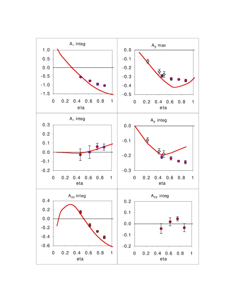
FIG. 15.: Energy dependence of the integrated spin correlation coefficients $\overline{A_{\Sigma}}$, $\overline{A_{\Delta}}$, $\overline{A_{zz}}$ $\overline{A_{xz}}$ and $\overline{A_{y0}}$, and the peak analyzing power $A_{y,max}$ for $\vec{p}\vec{p}\rightarrow pn\pi^{+}$. The diamond shape symbols represent measurements at lower energies and are taken from Ref. [18]. The solid lines are predictions of the Jülich meson exchange model. (There is no prediction for $A_{xz}$.)

C Deduction of important partial waves

The number of contributing partial waves grows rapidly with energy. If we restrict ourselves to Ss, Sp, Ps, and Pp contributions as above, the 19 individual amplitudes listed in Table IV are needed for a detailed interpretation of the data. There are 12 isoscalar and 7 isovector amplitudes. The experimental information available includes the three cross sections $\sigma_{tot},\ \Delta\sigma_{T}$, and $\Delta\sigma_{L}$ for $pp\rightarrow pn\pi^{+}\,$that are related to these amplitudes. In addition a recent $pp\rightarrow pp\pi^{0}\,$study provides the three relevant isovector cross sections $\sigma^{\prime}_{tot},\ \Delta\sigma^{\prime}_{T}$, and $\Delta\sigma^{\prime}_{L}$ (Ref. [26], Table V). As long as isospin is a good quantum number these cross sections also give the isovector part of the $pp\rightarrow pn\pi^{+}\,$reaction if taken at the same $\eta$.

So one has 6 new measurements for 19 variables. This necessitates some restriction of the further analysis. In a previous $pp\rightarrow pn\pi^{+}\,$study [18], closer to threshold, the partial wave space had been restricted to the lowest isoscalar amplitudes $a_{0},a_{1},a_{2}$, and to the lowest known isovector amplitudes. With this simplification and with reliance on the measured analyzing powers three amplitudes were deduced for $\eta\leq 0.5$. Some of these earlier results will be shown below. It will become apparent in comparison with our new data that the angular momentum space considered in Ref.[18] is too small for $\eta>0.3$. For $0.3<\eta<0.9$ it becomes necessary to consider all Ss, Sp, Ps, and Pp contributions. In order to reduce the number of variables we use similarities in the spin algebra coefficients for the 19 amplitudes of interest. A suitable combination of the 19 partial cross sections into six groups allows us to find the Sp and Ps strengths separately to deduce the lowest Pp isoscalar partial cross section for the amplitude $a_{3}$ directly, and to put a close upper limit on the Ss contributions. We will identify the isoscalar partial wave cross sections by $\sigma(a_{0}),\ \sigma(a_{1}),\ \sigma(a_{2}),\ \ldots$ and the isovector partial wave cross sections by $\sigma(b_{0}),\ \sigma(b_{1}),\ \sigma(b_{2}),\ \ldots$ as in Table V. Generally, $\sigma(a_{i})=C_{i}|a_{i}|^{2}$, where the $C_{i}$ factor is a combination of factors like $\pi$ and Clebsch-Gordan coefficients, which can differ from amplitude to amplitude. (Therefore the partial cross sections listed in Table V do not provide the magnitude of the corresponding amplitudes without further work.) The notation $\sigma(a_{1},a_{4\rightarrow 6})$ implies that we could not separate the cross sections for $a_{1}$, the Ss component, from the Pp components $a_{4}$ to $a_{6}$. Hence $\sigma(a_{1},a_{4\rightarrow 6})\equiv\sigma(a_{1})+\sigma(a_{4})+\sigma(a_{5})+\sigma(a_{6})$. The partial cross section groups that could be isolated are given in Eq. V C:

$${\rm Sp\ isoscalar\ terms:}\ \ \ \ \ \ \ \sigma(a_{0},a_{2}) = {\frac{1}{8}}\left({\Delta\sigma_{L}}+2{\Delta\sigma_{T}}+2{\sigma_{tot}}-{\Delta\sigma_{L}^{\prime}}-2{\Delta\sigma_{T}^{\prime}}-2{\sigma^{\prime}_{tot}}\right)$$ (51)

$${\rm Ps\ isovector\ terms:}\ \ \ \ \ \ \ \ \sigma(b_{1},b_{2}) = {\frac{1}{8}}\left({\Delta\sigma_{L}^{\prime}}+2{\Delta\sigma_{T}^{\prime}}+2{\sigma^{\prime}_{tot}}\right)$$ (52)

$${\rm Ss+Pp\ isoscalar\ terms:}\ \ \ \ \sigma(a_{1},a_{4\rightarrow 6}) = {\frac{1}{4}}\left(-{\Delta\sigma_{L}}+2\sigma_{tot}+{\Delta\sigma_{L}^{\prime}}-2{\sigma^{\prime}_{tot}}\right)$$ (53)

$${\rm Ss+Pp\ isovector\ terms:}\ \ \ \ \ \ \ \ \sigma(b_{0},b_{3}) = {\frac{1}{8}}\left({\Delta\sigma_{L}^{\prime}}-2{\Delta\sigma_{T}^{\prime}}+2{\sigma^{\prime}_{tot}}\right)$$ (54)

$${\rm Pp\ isoscalar\ terms:}\ \ \ \ \ \ \ \ \ \ \ \ \sigma(a_{3}) = {\frac{1}{8}}\left({\Delta\sigma_{L}}-2{\Delta\sigma_{T}}+2\sigma_{tot}-{\Delta\sigma_{L}^{\prime}}+2{\Delta\sigma_{T}^{\prime}}-2{\sigma_{tot}^{\prime}}\right)$$ (55)

$${\rm Pp\ isovector\ terms:}\ \ \ \ \ \ \ \sigma(b_{4\rightarrow 11}) = {\frac{1}{4}}\left(-{\Delta\sigma_{L}^{\prime}}+2{\sigma^{\prime}_{tot}}\right)$$ (56)

Of these six equations, which hold for $pp\rightarrow pn\pi^{+}\,$, three also hold for $pp\rightarrow pp\pi^{0}\,$. We note that Eq. V Cb has been presented before. It is identical to Eq. 13 in [26]. The six equations now permit a calculation of partial wave cross sections to the specified groups of final states from the measured spin-dependent cross sections. The sum of these partial cross sections equals the total $\pi^{+}$ production cross section. Since the partial cross sections add incoherently the effect of higher lying weak amplitudes is minimized. This is an advantage over relying on analyzing powers, which are sensitive to even small admixtures. The amplitudes included in each group are indicated on the left side of Eqs. V C.

In many experiments, including the present one, it is much easier to measure accurate cross section ratios than absolute cross sections. So our experimental $pp\rightarrow pn\pi^{+}\,$quantities are given as a fraction of the total $\pi^{+}$ production cross section $\sigma_{tot}$. The Eqs. V C are easily re-written in terms of partial wave strengths by dividing both sides by ${\sigma_{tot}}$. For the $p+\pi^{+}$ branch the values ${\Delta\sigma_{T}}/{\sigma_{tot}}$ and ${\Delta\sigma_{L}}/{\sigma_{tot}}$ were calculated from eqs. 4.6 and $A_{\Sigma}(\theta)$, $A_{\Delta}(\theta)$ and $\sigma_{0}(\theta)$. In figures and tables we will generally use the ratios of partial wave cross sections to total cross sections. We refer to them as partial wave strengths.

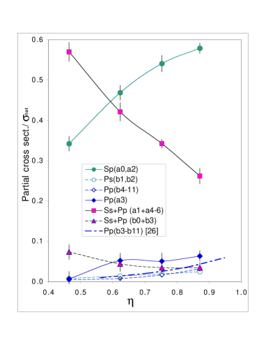
FIG. 16.: Partial wave strengths for six groups of amplitudes as function of $\eta$. The isoscalar cross sections are connected by solid lines, the isovector ones by dashed lines. The contributing amplitudes, including the (small) Pp contributions not resolved from the dominant Ss cross sections are indicated in the legend. The dash-dotted line represents the full Pp isovector strength contribution in $pp\rightarrow pn\pi^{+}\,$, as derived from the results of Ref. [26].

To use them in this study the total $pp\rightarrow pp\pi^{0}\,$and $pp\rightarrow pn\pi^{+}\,$cross sections were taken from the literature and interpolated for the present $\eta$ values. We obtained the $pp\rightarrow pp\pi^{0}\,$information needed from Ref. [26] and the $pp\rightarrow pn\pi^{+}\,$total cross sections from [18] and from Fig. 2 in Ref. [6]. The accuracy of the total cross section ratios so obtained is not very high, but it will suffice here because the isoscalar terms of interest are an order of magnitude larger than the isovector terms. The partial cross section strengths derived with Eqs. V C are displayed in Fig. 16 and listed in in Table V.

The primed cross sections are the (pure isovector) cross sections measured for $pp\rightarrow pp\pi^{0}\,$, which are also more accurately given as fractional strengths. To work in terms of $pp\rightarrow pn\pi^{+}\,$partial wave strengths the $pp\rightarrow pp\pi^{0}\,$strengths of Ref. [26] have to be multiplied by the ratio of the $pp\rightarrow pp\pi^{0}\,$and $pp\rightarrow pn\pi^{+}\,$unpolarized cross sections, taken at the same relevant $\eta$ values.

Fig. 16 shows the change of partial wave strength with energy for Sp, Ps, and other groups. It is immediately apparent that for the energy region studied the leading isoscalar partial cross sections are an order of magnitude larger than the isovector ones. It helps our discussion that lowest-lying Pp isoscalar partial wave strength Pp($a_{3}$) could be resolved. It is much smaller than the Ss and Sp strengths. So is the sum of all isovector cross sections for $\rm b_{4}\ to\ b_{11}$. The Pp strengths attributable to $b_{3}$ can be assessed by comparing Pp($b_{4\rightarrow 11}$) from this work with the heavy dash-dotted curve derived from [26] for the full Pp isovector strength Pp($b_{3\rightarrow 11}$).

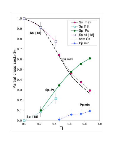
FIG. 17.: Sums of isoscalar and isovector partial wave strengths as function of $\eta$. The Sp+Ps sum is measured directly. The points labeled “Ss max” represent a close upper limit to the sum of the Ss partial cross sections. Any correction for the unresolved Pp amplitudes ($a_{4},a_{5},a_{6}$, and $b_{3}$) would lower the Ss curve (as indicated by the estimated errors). The admixtures can be expected to be smaller than $Pp(a_{3}$). The lower points show the documented Pp strengths only. The data at $\eta=0.22$ and 0.42 are from Ref. 18.

Therefore, it seems reasonable to assume that the Pp contributions from $a_{4},\ a_{5},a_{6}$ and $b_{3}$, which could not be disentangled from the the Ss amplitudes, are also much smaller than the Ss terms. On this basis we estimate that they make up no more than 5 to 10% of the “Pp entangled” $\rm Ss_{max}$ cross section curve. For $\eta=0.9$ the Sp($a_{0},a_{2})$ cross section has become dominant. As seen in Fig. 16, it is very much larger than the Ps isovector contribution. It would be of interest to resolve the isoscalar component $a_{0}$, because it can be used to constrain the strength of 3-body forces [13]. However, in this analysis $a_{0}$ and the much larger amplitude $a_{2}$ always appear together. The Ss fraction, including the unresolved Pp contributions, has fallen to less than 0.3. This is consistent with the work at 420 MeV [32].

In Fig. 17 the data points give the summed Sp+Ps strengths, the upper limit for the summed Ss strengths, and a lower limit for the Pp strength. The heavy dashed curve shows the likely energy dependence of the actual Ss strength. The divergence of the old and new $pp\rightarrow pn\pi^{+}\,$interpretation near $\eta\approx 0.45$ serves as a reminder that a partial wave analysis is only model independent if it fully encompasses all contributing amplitudes. This apparently was no longer true for the 320 MeV data ($\eta=0.42$) of Ref. 18.

In this respect our present difficulty to perfectly reproduce $A_{y}$ at 375 and 400 MeV in the Ss, Sp, Ps and Pp frame work (see Table II) should be taken as a warning. At these energies some higher partial waves may contribute enough so that they must be considered, at least for the analyzing powers.

VI Conclusions

We have measured the spin correlation coefficients $A_{\Sigma}$=$A_{xx}$+$A_{yy}$, $A_{\Delta}$=$A_{xx}$-$A_{yy}$, $A_{zz},A_{xz}$, and $A_{y}$, as well as angular distributions for $\sigma(\theta_{\pi})$ and the polarization observables $A_{ij}(\theta_{\pi})$ at energies from 325 to 400 MeV. At the lowest energies the results are in agreement with prediction of the Jülich meson exchange model. The agreement deteriorates considerably at energies where Ss transitions no longer dominate. At 375 and 400 MeV some physics aspects in $\vec{p}\vec{p}\rightarrow pn\pi^{+}$ apparently are missed by the model. This suspicion is supported by the even poorer agreement of the model with the $\vec{p}\vec{p}\rightarrow pp\pi^{0}$ data [26].

The $pp\rightarrow pp\pi^{0}\,$ and $pp\rightarrow pn\pi^{+}\,$ reactions are found to differ greatly in the relative importance of Sp, Ps, and Pp transitions. Sp strongly feeds the delta resonance in $pp\rightarrow pn\pi^{+}\,$, but this transition is forbidden for $\vec{p}\vec{p}\rightarrow pp\pi^{0}$. By contrast Ps contributions in $pp\rightarrow pn\pi^{+}\,$are no larger than Pp contributions, as seen in Fig. 16. In $\vec{p}\vec{p}\rightarrow pn\pi^{+}$ the Ss and Sp isoscalar terms are most important while the Pp transitions just begin to contribute. For $\vec{p}\vec{p}\rightarrow pp\pi^{0}$ Pp becomes dominant at $\eta=0.7$.

The partial wave analysis was able to reproduce almost all polarization observables within experimental errors. This supports the postulated adequacy of considering only Ss, Sp, Ps, and Pp transitions in the near threshold region. However, this angular momentum space may not be adequate to explain details of analyzing powers, because they can be affected by small admixtures of higher-lying transitions. Even in this limited space the number of individual partial waves for $\vec{p}\vec{p}\rightarrow pn\pi^{+}$ at 400 MeV is too large to deduce all individual amplitudes. Some interesting sum rules for groupings of amplitudes were found (Eqs. V C), and the corresponding partial cross sections could be extracted. They show, e.g., that for $\eta<1$ Pp and Ps terms play a considerably smaller role in $pp\rightarrow pn\pi^{+}\,$than in $pp\rightarrow pp\pi^{0}\,$.

Further progress may come from improved theoretical models that can accurately predict the new data at hand. It is interesting to note again that the Jülich model does well at 325 MeV where Ss dominates, but it increasingly fails for $pp\rightarrow pn\pi^{+}\,$(as well as for $pp\rightarrow pp\pi^{0}\,$) as higher angular momenta become important.

VII Acknowledgements

We acknowledge the assistance of Drs. M. Dzemidzic, F. Sperisen and D. Tedeschi in the early stages of the experiment. Throughout the runs we have benefitted from the helpful advice of Dr. W. Haeberli and the technical assistance of J. Doskow. We thank the IUCF accelerator operations group for their dedicated efforts. We are grateful to the authors of ref. [11] for making available to us calculations for $\vec{p}\vec{p}\rightarrow pn\pi^{+}$ obtained with their model.

This work was supported by the US National Science Foundation under Grants PHY95-14566, PHY96-02872, PHY-97-22556, PHY-99-01529, and by the department of Energy under Grant DOE-FG02-88ER40438.

VIII References

TABLE I.: Beam energies, integrated luminosities for the p + $\pi^{+}$ measurements, and the products of beam and target polarization for runs a and b. (No p+n data were taken in run a. The p+n measurements began in the middle of run b and have correspondingly lower integrated luminosities.)

	Run a			Run b
Energy	$\int L\,dt$	$P_{y}Q$	$\int L\,dt$	$P_{x}Q$	$P_{y}Q$	$P_{z}Q$
(MeV)	($nb^{-1}$)		($nb^{-1}$)
325.6	2.163	0.456 $\pm$0.003	3.0	0.059 $\pm$0.002	0.333 $\pm$0.002	0.296 $\pm$0.003
350.5	0.901	0.342 $\pm$0.004	1.3	0.053 $\pm$0.003	0.316 $\pm$0.003	0.267 $\pm$0.005
375.0	3.024	0.514 $\pm$0.004	4.1	0.041 $\pm$0.002	0.333 $\pm$0.002	0.266 $\pm$0.004
400.0	0.831	0.526 $\pm$0.006	1.1	0.039 $\pm$0.004	0.289 $\pm$0.004	0.203 $\pm$0.008

TABLE II.: Coefficients for the fits with Eqs. IV A that reproduce the measured angular distributions of the polarization observables. The associated Legendre polynomials used for the fits are determined by selection rules for Ss, Sp, Ps, and Pp transitions. The unpolarized angular distribution $\sigma_{0}(a_{00},b_{00})$ is given in arbitrary units by setting $a_{00}=1$. The errors listed refer to the individual fitting coefficients. The $\chi^{2}$ numbers give the overall quality of the fit to the data per degree of freedom. The fits are shown in Figs. 11, 13 and 14.

		325 MeV			350 MeV				375 MeV			400 MeV
Name	param.	param.	$\chi^{2}$	param.	param.	$\chi^{2}$	param.	param.	$\chi^{2}$	param.	param.	$\chi^{2}$
	value	error	data	value	error	data	value	error	data	value	error	data
$a_{00}$	1	-	-	1	-	-	1	-	-	1	-	-
$b_{00}$	0.168	0.035	-	0.190	0.040	-	0.199	0.030	-	0.196	0.045
$a_{\Sigma}$	-0.560	0.052	0.5	-0.810	0.055	0.6	-0.994	0.015	2.8	-1.070	0.024	1.4
$b_{\Sigma}$	-0.303	0.063		-0.478	0.067		-0.510	0.018		-0.439	0.029
$a_{\Delta}$	-0.037	0.091	1.4	-0.001	0.097	0.2	0.084	0.028	1.3	0.075	0.045	1.4
$b_{\Delta}$	-	-	-	-	-	-	-	-	-	-	-
$a_{zz}$	0.120	0.042	0.1	-0.177	0.047	0.8	-0.310	0.018	1.0	-0.431	0.037	3.1
$b_{zz}$	-0.188	0.054		-0.257	0.057		-0.233	0.021		-0.199	0.043
$a_{y0}$	-0.247	0.015	0.5	-0.255	0.013	0.9	-0.276	0.005	2.4	-0.285	0.008	3.9
$c_{y0}$	0.007	0.013		0.050	0.010		0.044	0.005		-0.032	0.007
$a_{xz}$	-0.051	0.042	0.7	0.021	0.042	1.2	0.053	0.021	1.1	-0.041	0.041	1.2
$c_{xz}$	0.106	0.038		0.047	0.036		-0.040	0.020		-0.104	0.036

TABLE III.: Beam energy, the $\eta$ parameter, and the deduced integrated spin correlation coefficients. The table gives the weighted average of all runs as shown in Fig. 15.

T(MeV)	$\eta$	$\overline{A_{\Sigma}}$	$\overline{A_{\Delta}}$	$\overline{A_{zz}}$	$\overline{A_{y0}}$	$\overline{A_{xz}}$
325.6	0.464	-0.533 $\pm$0.046	-0.027 $\pm$0.064	0.148 $\pm$0.041	-0.209 $\pm$0.011	-0.043 $\pm$0.044
350.5	0.623	-0.761 $\pm$0.046	0.001 $\pm$0.070	-0.143 $\pm$0.040	-0.218 $\pm$0.011	0.018 $\pm$ 0.036
375.0	0.753	-0.945 $\pm$0.068	0.062 $\pm$0.036	-0.283 $\pm$0.016	-0.237 $\pm$0.004	0.045 $\pm$0.019
400.0	0.871	-1.026 $\pm$0.023	0.056 $\pm$0.034	-0.414 $\pm$0.032	-0.244 $\pm$0.011	-0.035 $\pm$0.036

TABLE IV.: Angular momentum quantum numbers for the partial waves of the reaction $pp\rightarrow pn\pi^{+}\,$.

Type		Label	${}^{2s_{i}+1}l_{J}\rightarrow\kern 1.0pt^{2s_{f}+1}l_{p}j,l_{\pi}$
Ss	isoscalar	$a_{1}$	${}^{3}P_{1}\rightarrow^{3}\!S_{1},s$
Ss	isovector	$b_{0}$	${}^{3}P_{0}\rightarrow^{1}\!S_{0},s$
Sp	isoscalar	$a_{0}$	${}^{1}S_{0}\rightarrow^{3}\!S_{1},p$
		$a_{2}$	${}^{1}D_{2}\rightarrow^{3}\!S_{1},p$
Ps	isovector	$b_{1}$	${}^{1}S_{0}\rightarrow^{3}\!P_{0},s$
		$b_{2}$	${}^{1}D_{2}\rightarrow^{3}\!P_{2},s$
Pp	isoscalar	$a_{3}$	${}^{3}P_{0}\rightarrow^{1}\!P_{1},p$
		$a_{4}$	${}^{3}P_{1}\rightarrow^{1}\!P_{1},p$
		$a_{5}$	${}^{3}P_{2}\rightarrow^{1}\!P_{1},p$
		$a_{6}$	${}^{3}F_{2}\rightarrow^{1}\!P_{1},p$
Pp	isovector	$b_{3}$	${}^{3}P_{0}\rightarrow^{3}\!P_{1},p$
		$b_{4}$	${}^{3}P_{2}\rightarrow^{3}\!P_{1},p$
		$b_{5}$	${}^{3}P_{2}\rightarrow^{3}\!P_{2},p$
		$b_{6}$	${}^{3}F_{2}\rightarrow^{3}\!P_{1},p$
		$b_{7}$	${}^{3}F_{2}\rightarrow^{3}\!P_{2},p$
		$b_{8}$	${}^{3}P_{1}\rightarrow^{3}\!P_{0},p$
		$b_{9}$	${}^{3}P_{1}\rightarrow^{3}\!P_{1},p$
		$b_{10}$	${}^{3}P_{1}\rightarrow^{3}\!P_{2},p$
		$b_{11}$	${}^{3}F_{3}\rightarrow^{3}\!P_{2},p$

TABLE V.: Listing of the $pp\rightarrow pn\pi^{+}\,$partial wave strengths for the groups of isoscalar and isovector amplitudes indicated. The 300 MeV results listed were taken from Ref. [18]. The 300 MeV strengths not listed are assumed to be negligible.

Isoscalars
E(MeV)	$\eta$	Sp(a0,a2)	error	Ss+Pp (a1,a4-6)	error	Pp(a3)	error
300	0.220	0.088	0.030	0.740	0.050	-	-
325.6	0.464	0.342	0.018	0.570	0.024	0.006	0.018
350.5	0.623	0.469	0.018	0.421	0.023	0.052	0.018
375	0.753	0.541	0.020	0.342	0.011	0.050	0.020
400	0.871	0.579	0.013	0.262	0.019	0.063	0.013
Isosvectors
E(MeV)	$\eta$	Ps(b1,b2)	error	Ss+Pp (b0,b3)	error	Pp(b4-11)	error
300	0.220	-	-	0.173	0.022	-	-
325.6	0.464	0.007	0.002	0.073	0.007	0.004	0.003
350.5	0.623	0.014	0.003	0.044	0.005	0.007	0.002
375	0.753	0.019	0.002	0.034	0.003	0.016	0.002
400	0.871	0.024	0.003	0.034	0.004	0.031	0.004

REFERENCES

- [1] M. Gell-Mann and K. M. Watson, Ann. Rev. Nucl. Sci. 4, 219 (1954).
- [2] A. H. Rosenfeld, Phys. Rev. 96, 130 (1954).
- [3] D. Koltun and A. Reitan, Phys. Rev. 141, 1413 (1966).
- [4] M. E. Schillaci, R. R. Silbar and J. E. Young, Phys. Rev. 179, 1539 (1969).
- [5] H. O. Meyer et al., Phys. Rev. Lett. 65, 2846 (1990); see also, H. O. Meyer et al., Nucl. Phys. A539, 633 (1992).
- [6] W. W. Daehnick, S. A. Dytman, J. G. Hardie, W. K. Brooks, R. W. Flammang, L. Bland, W. W. Jacobs, T. Rinckel, P. V. Pancella, J.D. Brown and E. Jacobsen, Phys. Rev. Lett. 74, 2913 (1995).
- [7] C. Hanhart, J. Haidenbauer, A. Reuber, C. Schutz, and J. Speth, Phys. Lett. B 358, 21 (1995).
- [8] C. Hanhart, Ph.D. thesis, University of Bonn 1997.
- [9] C. Hanhart, J. Haidenbauer, M. Hoffmann, U.-G. Meissner, and J. Speth, Phys. Lett. B 424, 8 (1998).
- [10] C. Hanhart, J. Haidenbauer, O. Krehl, and J. Speth, Phys. Lett. B 444, 25 (1998).
- [11] C. Hanhart, J. Haidenbauer, O. Krehl, and J. Speth, Phys. Rev. C 61, 064008 (2000), and references therein.
- [12] T.-S. H. Lee and D. O. Riska, Phys. Rev. Lett. 70, 2237 (1993).
- [13] C. Hanhart, U. van Kolck, G. A. Miller, Phys. Rev. Lett. 85, 2905 (2000).
- [14] C. A. da Rocha, G. A. Miller and U. van Kolck, Phys. Rev. C 61, 034613 (2000).
- [15] B. Blankleider and A. N. Kvinikhidze, Few Body Syst. Suppl. 12, 223 (2000).
- [16] J. G. Hardie, S. A. Dytman, W. W. Daehnick, W. K. Brooks, R. W. Flammang, L. C. Bland, W. W. Jacobs, P. V. Pancella, T. Rinckel, J. D. Brown and E. Jacobsen, Phys. Rev. C 56, 20 (1997).
- [17] W. W. Daehnick, R. W. Flammang, S. A. Dytman, D. J. Tedeschi, R. A. Thompson, T. Vrana, C. C. Foster, J. G. Hardie, W. W. Jacobs, T. Rinckel, E. J. Stephenson, P. V. Pancella, W. K. Brooks, Phys. Lett. B 423, 213 (1998).
- [18] R. W. Flammang, W. W. Daehnick, S. A. Dytman, D. J. Tedeschi, R. A. Thompson, T. Vrana, C. C. Foster, J. G. Hardie, W. W. Jacobs, T. Rinckel, E. J. Stephenson, P. V. Pancella, W. K. Brooks, Phys. Rev. C 58, 916 (1998).
- [19] Swapan K. Saha, W. W. Daehnick, R. W. Flammang, J. T. Balewski, H. O. Meyer, R. E. Pollock, B. v. Przewoski, T. Rinckel, P. Thörngren-Engblom, B. Lorentz, F. Rathmann, B. Schwartz, T. Wise, P. V. Pancella, Phys. Lett. B 461, 175 (1999).
- [20] H. O. Meyer, L. D. Knutson, J. T. Balewski, W. W. Daehnick, J. Doskow, W. Haeberli, B. Lorentz, R. E. Pollock, P. V. Pancella, B. v. Przewoski, F. Rathman, T. Rinckel, Swapan K. Saha, B. Schwartz, P. Thörngren-Engblom, A. Wellinghausen, and T. Wise, Phys. Lett. B 480, 7 (2000).
- [21] L. D. Knutsen, Proceedings of the 4th International Conference on Nuclear Physics at Storage Rings, Indiana (1999), ed. H. O. Meyer and P. Schwandt, AIP Conference Proceedings No. 512 (AIP Melville, NY, 2000) p. 177
- [22] T. Rinckel, P. Thörngren-Engblom, H. O. Meyer, J. T. Balewski, J. Doskow, R. E. Pollock, B. v. Przewoski, F. Sperisen, W. W. Daehnick, R. W. Flammang, Swapan K. Saha, W. Haeberli, B. Lorentz, F. Rathmann, B. Schwartz, T. Wise, P. V. Pancella, Nucl. Inst. Meth. A 439, 117 (2000).
- [23] T. Wise, A. D. Roberts, and W. Haeberli, Nucl. Inst. Meth. A 336, 410 (1993). See also J. S. Price and W. Haeberli, Nucl. Instr. Meth. A 349, 321 (1994).
- [24] M. A. Ross et al., Nucl. Inst. and Meth. A 344, 307 (1994).
- [25] B. v. Przewoski et al., Phys. Rev. C 58, 1897 (1998).
- [26] H. O. Meyer, A. Wellinghausen, J. T. Balewski, J. Doskow, R. E. Pollock, B. v. Przewoski, T. Rinckel, P. Thörngren-Engblom, L. D. Knutson, W. Haeberli, B. Lorentz, F. Rathmann, B. Schwartz, T. Wise, W. W. Daehnick, Swapan K. Saha, P. V. Pancella, Phys. Rev. C 63, 064002 (2001).
- [27] W. W. Daehnick, W. K. Brooks, Swapan K. Saha and D. O. Kreithen, Nucl. Inst. and Meth. A 320, 290 (1992).
- [28] A. Del Guerra, Nucl. Inst. Meth. 135, 337 (1976).
- [29] B. Morton, E. E. Gross, E. V. Hungerford, J. J. Malanify, and A. Zucker, Phys. Rev. 169, 825 (1968).
- [30] B. v. Przewoski, J. T. Balewski, J. Doskow, H. O. Meyer, R. E. Pollock, T. Rinckel, P. Thörngren-Engblom, A. Wellinghausen, W. Haeberli, B. Lorentz, F. Rathmann, B. Schwartz, T. Wise, W. W. Daehnick, Swapan K. Saha, P. V. Pancella, Phys. Rev. C 61, 064604 (2000).
- [31] The computer code BMW was written by J. T. Balewski, H. O. Meyer, and A. Wellinghausen (unpublished).
- [32] R. G. Pleydon, W. R. Falk, M. Benjamintz, S. Yen, P.L. Walden, R. Abegg, D. Hutcheon, C. A. Miller, M. Hartig, K. Hicks, G. V. O’Rielly, and R. Shyam, Phys. Rev. C 59, 3208 (1999).