A new functional for charge and mass identification in $\Delta$E-E telescopes

Abstract

We propose a new functional for the charge and mass identification in $\Delta E-E$ telescopes. This functional is based on the Bethe formula, allowing safe interpolation or extrapolation in regions with low statistics. When applied to telescopes involving detectors delivering a linear response, as silicon detectors or ionization chambers, a good mass and charge identification is achieved. For other detectors, as caesium-iodide used as a final member of a telescope, a good accuracy is also obtained except in the low residual energy region. A good identification is however recovered if a non-linear energy dependence of the light output is included.

1 Introduction

Stacks of detectors, called telescopes, measuring the energy loss and residual energy of charged particles have been used for a long time to get charge and mass identification, and also energy, of such particles. Several combinations of detectors have been used for this purpose : ionization chambers, silicon detectors, plastic scintillators, thallium-activated caesium-iodide scintillators (CsI(Tl)) read by photomultipliers or photodiodes. The identification is obtained by plotting the energy loss in one or several components of the detector stack versus the residual energy released in the detector in which the particle has stopped. In such a plot events of a given charge and mass cluster around identification lines. Two methods can then be implemented to extract the identification for each event :

• interactive drawing of lines on top of ridges corresponding to a given charge or mass, or contours around events clustered around these ridges, any event being identified from its distance to ridge lines or its inclusion in one contour,

• fit of the ridge lines with a functional in which $Z$ and $A$ enter as parameters, the identification being obtained by inversion of the functional for given $\Delta E$ and $E$ in order to extract $Z$ and $A$.

Whereas the first method is probably more powerful and allows to face any situation, it suffers two main drawbacks : it doesn’t deliver any extrapolation in regions of low statistics, and it is human-time consuming because each identification line has to be accurately drawn. This last aspect becomes really a concern when multidetectors are used, in which hundreds of such telescopes are involved. The second method doesn’t suffer these inconveniences provided that the functional accurately models the data. Identification functionals have already been used in the past [1]. Due to their limited range of application, some extensions have been added later [2]. The purpose of this work is to propose a more complex functional based on physical grounds in order to allow accurate modelling of the data and safe extrapolations in regions where no data are present.

The second section is devoted to the derivation of a functional based on Bethe’s formula with a power law velocity dependence, and to its main properties. The third section proposes a phenomenological extension of this functional for data departing from the simple restriction of Bethe’s formula. In the fourth section we will show how the introduction of a non-linear term for the amplitude of the light of a CsI(Tl) crystal allows a good charge identification up to $Z=50$ for telescopes involving such detectors.

2 Basic functional

We assume that the stopping power of a fragment of energy ${\mathcal{E}}$, mass $A$ and nuclear charge $Z$ in a detecting medium takes the simple form :

$${\d{{\mathcal{E}}}\over\d X}={Z^{2}\over f({\mathcal{E}}/A)}$$ (1)

This formula can be straightly derived from Bethes’s formula [4] when the charge state inside the stopping medium is strictly equal to the nuclear charge $Z$. Its range of validity is restricted to light ions with energy sufficient to insure that they are fully stripped. In particular the Bragg zone of the stopping power curve, where the mean charge state is no more constant, is not addressed by this formula.

We also define the integral $F$ of $f$ as :

$$F(x)=\int\limits_{0}^{x}f(t)\,\d t$$ (2)

By integration of equation (1) one obtains the range-energy relation :

$$F({\mathcal{E}}/A)={Z^{2}\over A}X$$ (3)

This last relation can be applied to the case of telescopes made of a first detector of thickness $\Delta X$. The incoming fragment releases a part $\Delta E$ of its energy in this detector, and its residual energy $E$ in the rear detector for a residual range $X$.

When applied to the total energy and to the residual energy, relation (3) reads :

$$\left\{\begin{array}[]{rcl}\displaystyle{Z^{2}\over A}(X+\Delta X)&=&F\left(\displaystyle{E+\Delta E\over A}\right)\\ \displaystyle{Z^{2}\over A}X&=&F\left(\displaystyle{E\over A}\right)\end{array}\right.$$

which, by elimination of $X$, delivers the $E$-$\Delta E$ relation :

$$\Delta E=A\left\{F^{-1}\left[F(E/A)+{Z^{2}\over A}\Delta X\right]-{E\over A}\right\}$$ (5)

This formula is rigorous as long as the stopping power takes the form (1). However to reach a practical use we need to specify the function $f$. We will choose a form close to Bethe’s behaviour but simpler in order to obtain and analytical form of the integral inverse $F^{-1}$.

2.1 Specialisation of the function $f$

In the case of Bethe’s formula in the non-relativistic domain, $f({\mathcal{E}}/A)$ is almost proportional to ${\mathcal{E}}/A$ because the logarithmic term can be considered as constant. Therefore we will choose a power law dependence :

$$f({\mathcal{E}}/A)=({\mathcal{E}}/A)^{\mu}$$ (6)

with $\mu\approx 1$. This particular form of $f$ is advantageous because it leads to an analytical form of (5) which reduces to :

$$\Delta E=\left[E^{\mu+1}+(\mu+1)Z^{2}A^{\mu}\,\Delta X\right]^{1\over\mu+1}-E$$ (7)

One can notice that this relation is strictly equivalent to the functional used in [1] because both are based on the same hypotheses.

2.2 Properties of the $E$-$\Delta E$ relation

By taking the derivative of expression (7) versus $E$ at $E=0$ one gets the slope at the starting point of the identification line which turns out to be equal to -1 independently of $Z$ and $A$. For signals delivered by real detectors this slope includes the ratio of electronic gains. However, in case of detectors exhibiting a linear response as silicon detectors, this constancy of the starting slope is generally achieved. Conversely the verification of this property is a good indication of the validity of approximations brought by (1).

By setting $E=0$ in (7) one obtains the series of crossing points of identification lines with the energy loss axis :

$$\Delta E_{0}=\left[(\mu+1)\,\Delta X\right]^{1\over\mu+1}Z^{2\over\mu+1}A^{\mu\over\mu+1}$$ (8)

In particular for $\mu=1$, close to reality, these starting energy losses are proportional to $Z\sqrt{A}$.

At high energy the second term between $[\ldots]$ in equation (7) becomes small, compared to the first one, and an expansion to first order can be performed :

$$\Delta E_{\infty}=\Delta X{Z^{2}\over(E/A)^{\mu}}$$ (9)

which is proportional to the stopping power, as expected.

2.3 Power law functional

If we assume that the detector response is linear, and that data comply to relation (7), then they should be fitted by the following function :

$$\Delta E=\left[(gE)^{\mu+1}+\left(\lambda\,Z^{2\over\mu+1}A^{\mu\over\mu+1}\right)^{\mu+1}\right]^{1\over\mu+1}-gE$$ (10)

where the parameters are $g$ (ratio of electronic gains), $\lambda$ which includes the thickness of the first detector and $\mu$ which is close to 1. Furthermore $E$ and $\Delta E$ are net signals from which pedestals have been subtracted. We then obtain a 3-parameter formula, or a 5-parameter formula if we also fit on the $\Delta E$ and $E$ pedestals.

To guarantee a convergence of the fit in all situations one should provide reasonable starting values and impose constraints on the range of the parameters. In particular $\mu$ should lie between 0.5 and 1.5 with a starting value $\mu_{0}=1$, the initial value $\lambda_{0}$ of $\lambda$ should be determined from the starting point of an identification line, and $g_{0}$ should be obtained from the slope at the same point. The reader is referred to the appendix for technicalities related to the fit procedure.

Once parameters have been determined by the fitting procedure, the function (10) can be used to extract $Z$ and eventually $A$ associated to any $\Delta E-E$ pair. This is achieved by an analytical inversion of equation (10) which delivers the quantity $Z^{2}A^{\mu}$ as early observed [1]. If one is only interested in the charge identification $A$ is set dependent on $Z$, the simplest prescription being $A=2Z$, and equation (10) is solved for $Z$ and the solution is projected onto the nearest integer number $Z_{i}$. Furthermore if the mass identification is required, the value $Z_{i}$ is taken for $Z$ and the equation is solved for $A$.

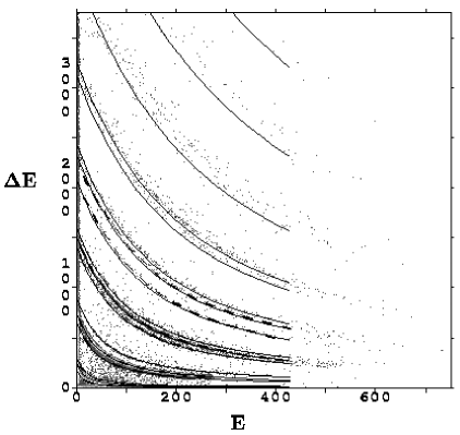
Figure 1: $\Delta E-E$ map from a silicon-silicon telescope. The 8 dashed lines, from hydrogen to beryllium, are the reference lines used for the 5-parameter fit of equation (10), which in turn generates the thin continuous lines. For $Z=6,7,8$, $A=2Z$ is assumed.

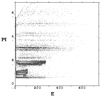
Figure 2: Plot of the particle identification variable defined as $PI=Z_{i}+0.2(A-2Z_{i})$ where $Z_{i}$ is the nearest integer deduced from the functional (10) setting $A=2Z$, and $A$ is the mass which solves (10) when $Z=Z_{i}$.

As an example figure 1 shows the $\Delta E-E$ map obtained with a calibration module of INDRA, made of a silicon detector of thickness 70 $\mu$m and a lithium-diffused silicon detector 2 mm thick, placed in front of a CsI(Tl) crystal used as a veto removing all particles punched through the silicon-lithium detector. The 8 dashed lines are the reference lines, from hydrogen to beryllium, used as references for the 5-parameter fit. The result of the fit is shown on figure 2 which displays the particle identification $PI=Z_{i}+0.2(A-2Z_{i})$ versus the energy released in the silicon-lithium detector. In can be verified that distorsions are very small and that the extrapolation toward boron an carbon elements is correct, indicating that the power law formula models correctly the data in this range.

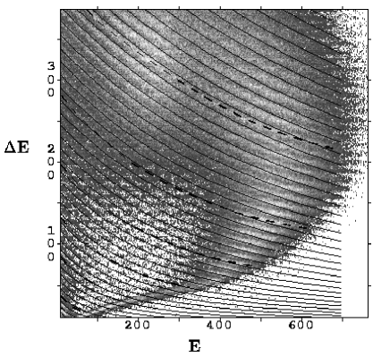
Figure 3: $\Delta E-E$ map obtained with a 150 $\mu$m-750 $\mu$m silicon telescope for the ²⁰⁸Pb+^natSi reaction at 29 MeV/n [8]. More populated areas are indicated by clearer zones. Thick dashed lines drawn for $Z=8,13,17,22,28,37$ are used as a reference for the 5-parameter fit with relation (10) which generates the thin lines.

However it has already been noticed in the past [2, 3] that for a wider $Z$ range, the above formula must be extended. The stopping power may depart from the behaviour ruled by relations (1) and (6), moreover the response of some detectors is not completely linear : pulse height defect in silicon detectors, light response of CsI(Tl)  detectors$\ldots$ Figure 3 shows the $\Delta E-E$ map obtained with a telescope made of 2 silicon detectors, of thicknesses equal to 150 $\mu$m and 750 $\mu$m, in the case of a ²⁰⁸Pb beam at 29 MeV/n [8]. Thick dashed lines drawn on top of ridges associated to $Z=8,13,17,22,28,37$ are used as a reference for the 5-parameter fit with relation (10) which generates the thin lines. It turns out that the functional hardly reproduces the data in the whole range : not only its $Z$ dependence is approximative, but also the shape of the energy dependence for a given line.

Therefore an enrichment of (10) is highly desired in order to benefit from more degrees of freedom. The extension proposed hereafter is not based on theoretical considerations but rather on phenomenological requirements.

3 Extended functional

One can see from equation (10) that $\mu$ rules the ordinates of starting points of identification lines. Once $\mu$ has been fitted to reproduce these data, the rapidity of the transition from the low energy domain dominated by $\displaystyle\lambda\,Z^{2\over\mu+1}A^{\mu\over\mu+1}$ to the high energy region, proportional to the stopping power, is fixed. This could lead to a too strong constraint when applied to real data. One could introduce an additional parameter for the $Z$ exponent but this would still link the $Z$ dependencies in the low and high energy regions. As regards the $A$ exponent, it can’t be touched because it insures the right asymptotic behaviour at high energy, toward the stopping power.

The ideal solution should meet the following prescriptions : independent variations in $Z$ and $A$ in the low and high energy regimes, possibility of tuning separately the rapidity of the transition between these regimes, correct asymptotic behaviour at high energy. This is achieved by the addition of new phenomenomogical term.

We define the extended functional as :

$$\Delta E=\left[(gE)^{\mu+\nu+1}+\left(\lambda Z^{\alpha}A^{\beta}\right)^{\mu+\nu+1}+\xi Z^{2}A^{\mu}(gE)^{\nu}\right]^{1\over\mu+\nu+1}-gE$$ (11)

which reduces to the basic functional (10) when one substitutes $\mu$ for $\mu+\nu$ and sets $\alpha=2/(\mu+1)$, $\beta=\mu/(\mu+1)$ and $\xi=0$, or even more simply if one sets : $\nu=0$ and $\lambda=0$.

The $g$ parameter still represents the slope of identification lines at their starting points (at $E=0$), equal for all lines as for the power law formula. The energy loss value at the starting points writes : $\Delta E_{0}=\lambda Z^{\alpha}A^{\beta}$, showing that this series of points essentially determines the $\lambda$, $\alpha$ and $\beta$ parameters.

At higher energies an expansion of (11) to first order can be carried out, leading to :

$$\Delta E_{\infty}={1\over\mu+\nu+1}\times{1\over(gE/A)^{\mu}}\times\left[\xi Z^{2}+{(\lambda Z^{\alpha})^{\mu+\nu+1}A^{\beta(\mu+\nu+1)-(\mu+\nu)}\over(gE/A)^{\nu}}\right]$$

One can notice that at high energy the $\displaystyle{\d E/\d X}$ is recovered if $\mu$ stays in the vicinity of 1, and that $\xi$ governs the amount of energy loss in this region. Moreover one benefits from the second term inside the square brackets which allows, through the $\nu$ parameter, to change the shape of curves in the region of intermediate energy.

The extended formula is a 7-parameter functional ($\lambda$, $\alpha$, $\beta$, $\mu$, $\nu$, $\xi$ and $g$) or a 9-parameter one if both pedestals are also considered as parameters of the fit. The convergency of the fit is always insured only if good starting values are supplied and if constraints are applied to the range of parameters. More precisely one should adopt : $\alpha_{0}=\mu_{0}=1$, $\beta_{0}=0.5$, $\nu_{0}=1$, $\lambda_{0}$ determined from the starting point of an identification line, $g_{0}$ from its starting slope, and $\xi_{0}$ from one point taken at high energy. The ranges should be restricted to :  $0.5<\alpha<1.5$, $0.2<\beta<1$, $0.2<\mu<1.5$,  $0.1<\nu<4$,  $\lambda_{0}/4<\lambda<4\lambda_{0}$,  $g_{0}/4<g<4g_{0}$, $0<\xi$. In the case where no mass identification is given, the number of parameters is decremented by one : $\beta$ is kept equal to 0.5 and $A$ is taken as a function of $Z$, the simplest relationship being $A=2Z$.

Unlike the power law formula, the extended formula can’t be analytically inverted to extract $Z$ and $A$ from a $\Delta E-E$ pair. This can only be done numerically and the fastest algorithm is probably the Newton-Raphson method which however needs the derivatives of (11) with respect to $Z$ and $A$.

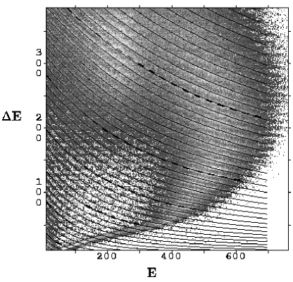
Figure 4: Same as figure 3 but thin lines result now from the fit based on the 8-parameter extended functional (11), assuming $A=2Z$.

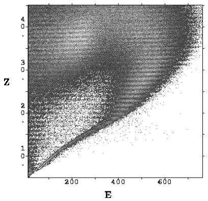
Figure 5: For the same data as in figures 3 and 4, the $Z$ extracted from relation (11) is plotted versus the residual energy to exhibit possible distorsions.

The quality of a fit based on this extended formula with 8 parameters, assuming $A=2Z$ and $\beta$ arbitrarily set, is shown on figure 4 where it appears that the shape of the curves is nicely reproduced, and also the interpolation in regions where no reference line guides the fit procedure. Even the extrapolation toward higher $Z$’s is satisfactory, having in mind that in this region the simple hypothesis $A=2Z$ is unlikely to hold. Figure 5 shows that only small distorsions remain when the identified $Z$ for each event is plotted versus the residual energy.

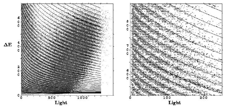
Figure 6: $\Delta E-h$ plot for a silicon-CsI(Tl) telescope, the abscissa is the total light output reconstructed from the fast and slow components of the CsI(Tl). The thick dashed lines follow the ridges of charges $Z=4,6,12,22,30,40$ and the thin lines result from the 8-parameter fit based on the extended functional (11) with $A=2Z$. The right part is a zoom applied to the low light region of the left map, including the line $Z=30$. The non-linearity of the light response shows up by the high curvature of data, not predicted by the functional.

We can also check the ability of this functional to reproduce the data for telescopes using a CsI(Tl) crystal as a stopping detector, for which the light response is not linear with the deposited energy and depends on the nature of the particle. For this purpose we worked on the data collected by a module of the second ring of the multidetector INDRA, made of a 300 $\mu$m silicon planar detector followed by a CsI(Tl) of depth equal to 14 cm [9]. As the CsI(Tl)  signal was only partially integrated on 2 time intervals for the delivering of the so-called slow and fast components, we didn’t have at disposal a true measurement of the total light signal, integrated over the duration of the pulse. We reconstructed this total light signal $h$ by a combination of slow and fast components following a procedure described in [7]. Figure 6 is an illustration of a $\Delta E-h$ plot collected with a tin beam. The thick dashed lines are drawn on top of charges $Z=4,6,12,22,30,40$ and the thin lines result from the 8-parameter fit with $A=2Z$. Despite the non-linearity of the light response and its dependence with $Z$ the fit is in good agreement with the data, showing that the parameters of the functional are able to partially compensate for these effects. However by looking carefully at the low residual energy region, as displayed in the right part of figure 6, one can see that the curvature of data is much more pronounced than predicted by the functional. This effect is due to the highly non-linear light response which is almost quadratic in this region. Any improvemevent of the accuracy of generated identification lines in this region needs an explicit inclusion of such a non-linearity.

4 Light response of caesium-iodide crystal

The idea for a new extension of functionals (10) and (11) is to substitute for $E$ its evaluation from the light output, in order to derive direct dependencies of the energy loss with the light output, the most part of non-linearities being carried by the relationship between light and energy.

We will take for the light response of CsI(Tl) crystals a dependence deduced from the Birks formula [5]. If one denotes $h$ the net light output after subtraction of the pedestal, its dependence with the energy deposition takes the form [6] :

$$h=E-\rho\ln{\left(1+{E\over\rho}\right)}\qquad\hbox{where}\qquad\rho=\eta Z^{2}A$$ (12)

and $\eta$ is a new parameter. No multiplicative constant is needed because the scaling factor is already included in the $g$ parameter of the functional, this is equivalent to consider the energy and the light output as measured with the same unit. This formula is not the most accurate [7] and particularly it discards the loss of quenching due to the delta electrons. We take it merely as a reasonable way of accounting for the non-linearities at low energy and high $Z$, hoping that the other parameters of the functional will be able to compensate its partial inadequacy.

However one difficulty arises from the fact that equation (12) cannot be analytically inverted to express $E$ as a function of $h$, as required for its insertion into the functionals (10) or (11). This is the reason why we adopted a slightly different formula for the inverse relation, imposing the same asymptotic behaviours at low and high energy. From (12) we derive for the low and high energy regimes :

$$E\longrightarrow 0 \qquad\Longrightarrow\qquad h\longrightarrow{E^{2}\over 2\rho}$$

$$E\longrightarrow\infty \qquad\Longrightarrow\qquad h\longrightarrow E-\rho\ln{\left(E\over\rho\right)}$$

which exhibits the quadratic dependence at low energy. By inverting these relations one gets :

$$h\longrightarrow 0 \qquad\Longrightarrow\qquad E\longrightarrow\sqrt{2\rho h}$$

$$h\longrightarrow\infty \qquad\Longrightarrow\qquad E\longrightarrow h+\rho\ln{\left(h\over\rho\right)}$$

Now we seek for a formula which complies with the above limiting behaviours, and we can check that :

$$E=\sqrt{h^{2}+2\rho h\left[1+\ln{\left(1+{h\over\rho}\right)}\right]}$$ (13)

fulfills this condition. Obviously relation (13) is not the strict inverse of (12), but it departs from it by 7.4 % only at maximum, and both become identical at low and high energy.

If we use this relation in combination with (11), we obtain now a functional with 8 parameters ($\lambda$, $\alpha$, $\beta$, $\mu$, $\nu$, $\xi$, $g$ and $\eta$), and 2 eventually additional parameters if pedestals in $h$ and $\Delta E$ are also adjusted.

Figure 7: Same as figure 6 but the thin lines result now from a 9-parameter fit combining relations (11) and (13). The curvature of data at low energy is now reproduced.

Figure 7 displays the calculated lines resulting from a 9-parameter fit in which $\beta$ has been kept constant as the charge identification only is given, and $A=2Z$ is assumed. It can be seen that a satisfactory agreement is obtained for the shape of the curves. Particularly one can notice that the high curvature of the lines in the vicinity of the energy loss axis is well reproduced by the introduction of the light response and its quadratic dependence at low energy. Furthermore a stable extrapolation is deduced for the charges higher than 40, the highest line used as a reference for the fit.

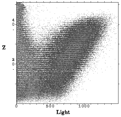
Figure 8: For the same data as in figures 6 and 7, the $Z$ extracted from relations (11) and (13) is plotted versus the residual energy to exhibit possible distorsions.

The quality of the charge identification can be checked on figure 8 where the distorsions of the identified $Z$ versus the light output appear to be small even for a wide range of charges. The apparent loss of resolution at low $Z$’s simply reflects the coding granularity, the channel size in energy loss becoming too large for these low charges.

5 Conclusion

Starting from the usual power law formula we propose an extended functional for the particle identification in $\Delta E-E$ telescopes, allowing a good mass and charge identification with silicon detectors on a wide range in energy and charge. Its domain of applicability remains however limited to situations where the Bragg region plays a minor role, in particular this excludes high $Z$’s detected in thin $\Delta E$ detectors. This functional can also be applied to specific cases where the $E$ signal is no longer linear with the energy deposition, as for example for silicon-CsI(Tl) telescopes in which the fast component of the CsI(Tl) is taken as a measure of the residual energy. This procedure has been applied to the calibrating modules in the INDRA multidetector, however it appears to be accurate only on a range of a few charges. By using the total light output of CsI(Tl), either by integrating the whole light signal or by estimating it from the partial integrations associated to the slow and fast components, the agreement between data and the extended formula is highly improved on a large range of $Z$. Moreover the discrepancies which remain at low residual energy are removed by the explicit introduction of the non-linear light response of the CsI(Tl) crystal, and a good quality of the identification is obtained on a wide range in charge and energy. This new functional opens the possibility of identifying particles in silicon or silicon-CsI(Tl) telescopes by defining only a limited number of reference points, and allows to rely on the deduced interpolation and even on the extrapolation in low statistics regions. It should make easier the usual identification task of particle identification in the case of charged particle multidetectors. The author expresses his aknowledgement to M. Morjean and to the INDRA collaboration, for having provided their data before publication.

Appendix A Appendix

The fit algorithm relies on the local quadratic expansion of the $\chi^{2}$. At each step a calculation is made for $\chi^{2}$, its gradient, and an estimation of the hessian matrix obtained by neglecting the second derivatives of the functional. This approximation is powerful because it always delivers a definite positive matrix which, in the vicinity of the minimum, becomes very close to the true hessian matrix. With such a prescription it is necessary to compute only the functional value and its gradient at each data point. The minimization proceeds iteratively and at each step the status of constraints is checked.

In order to insure a correct convergency 2 conditions have to be met :

• good starting values of the parameters have to be supplied as already explained,

• for the minimization procedure the parameters have to be scaled in order to be of the order of unity.

For a practical use, the formulas giving the derivatives of the functional (11) against parameters are written hereafter. By denoting :

$$G=\left[(gE)^{\mu+\nu+1}+\left(\lambda Z^{\alpha}A^{\beta}\right)^{\mu+\nu+1}+\xi\,Z^{2}A^{\mu}(gE)^{\nu}\right]$$

the derivatives can be expressed as :

$${\partial\Delta E\over\partial\lambda} = G^{{1\over\mu+\nu+1}-1}\left(\lambda Z^{\alpha}A^{\beta}\right)^{\mu+\nu+1}{1\over\lambda}$$

$${\partial\Delta E\over\partial\alpha} = G^{{1\over\mu+\nu+1}-1}\left(\lambda Z^{\alpha}A^{\beta}\right)^{\mu+\nu+1}\ln{\left(Z\right)}$$

$${\partial\Delta E\over\partial\beta} = G^{{1\over\mu+\nu+1}-1}\left(\lambda Z^{\alpha}A^{\beta}\right)^{\mu+\nu+1}\ln{\left(A\right)}$$

$${\partial\Delta E\over\partial g} = \left\{G^{{1\over\mu+\nu+1}-1}{1\over gE}\left[(gE)^{\mu+\nu+1}+{\nu\over\mu+\nu+1}\xi\,Z^{2}A^{\mu}(gE)^{\nu}\right]-1\right\}\,E$$

$${\partial\Delta E\over\partial E} = \left\{G^{{1\over\mu+\nu+1}-1}{1\over gE}\left[(gE)^{\mu+\nu+1}+{\nu\over\mu+\nu+1}\xi\,Z^{2}A^{\mu}(gE)^{\nu}\right]-1\right\}\,g$$

$${\partial\Delta E\over\partial\mu} = {G^{{1\over\mu+\nu+1}-1}\over\mu+\nu+1}\left\{(gE)^{\mu+\nu+1}\ln{\left(gE\right)}+\left(\lambda Z^{\alpha}A^{\beta}\right)^{\mu+\nu+1}\ln{\left(\lambda Z^{\alpha}A^{\beta}\right)}+\vphantom{1^{1}\over 1}\right.$$

$$\mbox{\hskip 56.9055pt}\left.\xi\,Z^{2}A^{\mu}(gE)^{\nu}\ln{\left(A\right)}-{G\ln{\left(G\right)}\over\mu+\nu+1}\right\}$$

$${\partial\Delta E\over\partial\nu} = {G^{{1\over\mu+\nu+1}-1}\over\mu+\nu+1}\left\{(gE)^{\mu+\nu+1}\ln{\left(gE\right)}+\left(\lambda Z^{\alpha}A^{\beta}\right)^{\mu+\nu+1}\ln{\left(\lambda Z^{\alpha}A^{\beta}\right)}+\vphantom{1^{1}\over 1}\right.$$

$$\mbox{\hskip 56.9055pt}\left.\xi\,Z^{2}A^{\mu}(gE)^{\nu}\ln{\left(gE\right)}-{G\ln{\left(G\right)}\over\mu+\nu+1}\right\}$$

$${\partial\Delta E\over\partial\xi} = {G^{{1\over\mu+\nu+1}-1}\over\mu+\nu+1}Z^{2}A^{\mu}(gE)^{\nu}$$

$${\partial\Delta E\over\partial Z} = G^{{1\over\mu+\nu+1}-1}\left\{{\alpha\,\left(\lambda Z^{\alpha}A^{\beta}\right)^{\mu+\nu+1}+{2\over\mu+\nu+1}\xi\,Z^{2}A^{\mu}(gE)^{\nu}\over Z}\right\}$$

$${\partial\Delta E\over\partial A} = G^{{1\over\mu+\nu+1}-1}\left\{{\beta\,\left(\lambda Z^{\alpha}A^{\beta}\right)^{\mu+\nu+1}+{\mu\over\mu+\nu+1}\xi\,Z^{2}A^{\mu}(gE)^{\nu}\over A}\right\}$$

The derivative ${\partial\Delta E/\partial E}$ is involved in the $E$-pedestal dependence. It is also useful when $E$ is expressed from the light output using (13). The ${\partial\Delta E/\partial Z}$ and ${\partial\Delta E/\partial A}$ derivatives are ingredients of the Newton-Raphson method for the determination of $Z$ and $A$ for a given $\Delta E-E$ pair whence the parameters have been determined.

Regarding the light response (13), the useful derivatives are :

$${\partial E\over\partial h} = {h\over E}\left\{1+{1\over 1+h/\rho}+{1+\ln{\left(1+h/\rho\right)}\over h/\rho}\right\}$$

$${\partial E\over\partial\rho} = {h\over E}\left\{{1\over 1+h/\rho}+\ln{\left(1+h/\rho\right)}\right\}$$

References

- [1] F. S. Goulding, D. A. Landis, J. Cerny and R. H. Pehl, Nucl. Instr. and Meth. 31 (1964) 1
- [2] G. W. Butler, A. M. Poskanzer and D. A. Landis, Nucl. Instr. and Meth. 89 (1970) 189
- [3] T. Shimoda, M. Ishihara, K. Nagatani and T. Nomura Nucl. Instr. and Meth. 165 (1979) 261
- [4] M. S. Livingston and H. A. Bethe, Rev. Mod. Phys. 9 (1937) 245
- [5] J. B. Birks, The Theory and Practice of Scintillation Counting (Pergamon 1964) 439
- [6] D. Horn, G. C. Ball, A. Galindo-Uribarri, E. Hagberg and R. B. Walker, R. Laforest and J. Pouliot, Nucl. Instr. and Meth. A320 (1992) 273
- [7] M. Pârlog, B. Borderie, M. F. Rivet, G. Tăbăcaru, A. Chbihi, M. Elouardi, N. Le Neindre, O. Lopez, E. Plagnol, L. Tassan-Got, and the INDRA collaboration, Nucl. Instr. and Meth. A to be published
- [8] M. Morjean, Private communication
- [9] J. Pouthas et al., Nucl. Instr. and Meth. A357 (1995) 418