Magnetic trapping of ultracold neutrons

Abstract

Three-dimensional magnetic confinement of neutrons is reported. Neutrons are loaded into an Ioffe-type superconducting magnetic trap through inelastic scattering of cold neutrons with ⁴He. Scattered neutrons with sufficiently low energy and in the appropriate spin state are confined by the magnetic field until they decay. The electron resulting from neutron decay produces scintillations in the liquid helium bath that results in a pulse of extreme ultraviolet light. This light is frequency downconverted to the visible and detected. Results are presented in which $500\pm 155$ neutrons are magnetically trapped in each loading cycle, consistent with theoretical predictions. The lifetime of the observed signal, $660~{}\mathrm{s}~{}^{+290}_{-170}$ s, is consistent with the neutron beta-decay lifetime.

I Introduction

The beta-decay lifetime of the neutron is of interest in a number of contexts. It has a direct impact on cosmological modeling as an input to the calculation of the production of light elements during the Big Bang. The isotopic ratios measured in extragalactic gas clouds (in which isotopic abundances are thought to have remained constant since the Big Bang) can be compared to Big Bang Nucleosynthesis calculations in order to place limits on the ratio of baryons to photons in the early universe. In the calculation of the expected ⁴He/¹H ratio, the dominant uncertainty is the lifetime of the neutron[1, 2].

Beta decay of the neutron is both the simplest nuclear beta decay, and more generally, the simplest of the charged-current weak interactions in baryons. Measurements of the weak interaction parameters can be obtained using neutron beta decay with fewer and simpler theoretical corrections than measurements using the beta decay of nuclei. The neutron beta decay rate is proportional to the quantity $g_{v}^{2}+3g_{a}^{2}$ where $g_{v}$ and $g_{a}$ are the semileptonic vector and axial-vector coupling constants. To extract the coupling constants uniquely from neutron beta-decay measurements requires either an independent measurement of $g_{v}$ or $g_{a}$ or of the (more experimentally accessible) ratio $g_{a}/g_{v}\equiv\lambda$.

The technique of magnetic trapping offers the promise of significant improvements over previous measurements in the accuracy of the neutron lifetime ($\tau_{n}$). Past measurements have relied on two techniques for measuring $\tau_{n}$: beam and closed-sample type measurements. At present, both techniques appear to be systematically limited at the $10^{-3}$ level.

In a beam measurement, a well collimated cold neutron beam passes continuously through a decay region of known volume. Each neutron decay occurring in that volume is counted. At the end of the decay region, the flux of the neutron beam is measured with a 1/$v$ weighting, where $v$ is the velocity. The neutron lifetime is ideally given by the ratio of the number of decays per unit time to the number of neutrons in the decay region. In the most precise measurement to date using this method ($\tau_{n}=889.2~{}\mathrm{s}\pm 4.8$ s [3, 4]), neutron decays were counted by detecting the decay protons and the beam flux was measured by detecting $\alpha$-particles emitted in the $n+\mathrm{{}^{10}B}\rightarrow\mathrm{{}^{7}Li}+\alpha$ reaction. Of the 4.8 s uncertainty, 3.4 s is attributed to systematic effects in the measurement of the neutron flux. An improved version of this experiment (presently running at the National Institute of Standards and Technology, NIST) aims for an accuracy of less than two seconds[5].

In the closed-sample measurements, neutrons with energies lower than the interaction potential of the material (i.e. ultracold neutrons or UCN) are loaded into a physical box and stored (via total reflection of the neutrons from the material surfaces) for a variable length of time before being counted. The neutron lifetime can be extracted from the dependence of the detected neutron population on the storage time. Several storage techniques have been used to make measurements of the neutron lifetime. The most precise storage measurements yielded values of $\tau_{n}=882.6~{}\mathrm{s}\pm 2.7$ s[6], $888.4~{}\mathrm{s}\pm 3.3$ s[7] and $885.4~{}\mathrm{s}\pm 0.9~{}s\pm 0.4$ s[8].

Experiments using this storage technique to measure the neutron lifetime measure the total rate at which neutrons are lost from the storage vessel, both by beta decay and by any other loss mechanisms. The accuracy of the lifetime measurement is limited either by unknown loss mechanisms or by the uncertainty in corrections for large loss mechanisms which arise from the interactions between the stored neutrons and the walls of the storage vessel. Most experiments use storage data to extrapolate to the ideal case of no wall losses. In Ref. [6], the physical size of the storage vessel is varied, and the measurements are extrapolated to an infinite volume. In Ref. [7], the storage time is measured as a function of UCN velocity, and an extrapolation is made to zero velocity, or an infinite time between collisions with the walls. The most recent measurement, [8], uses two different storage-vessel sizes with neutron detectors to measure the relative rate at which neutrons are scattered out of the storage vessel in the two configurations.

A second storage technique uses the interaction of the magnetic moment of the neutron with magnetic field gradients. This technique was first discussed by Vladimirski$\mathrm{\breve{i}}$ in 1961[9], just two years after Zeldovich first discussed material storage[10]. Since that time there have been several experiments to store neutrons magnetically with varying degrees of success[11, 12, 13, 14].

In the NESTOR (NEutron STOrage Ring) experiment, neutrons in a range of velocities from 6 m s^-1 to 20 m s^-1 were stored in a sextupole magnetic storage ring analogous to the storage rings used at particle accelerators[12, 14]. Magnetic field gradients reflect neutrons at a glancing incidence, storing neutrons in certain trajectories. The storage ring technique relies on the stored neutrons to remain in these trajectories. Neutron loss from these trajectories (attributed to betatron oscillation) limited this measurement.

Three-dimensional magnetic trapping was later attempted with a spherical hexapole trap[13]. The lack of neutrons trapped in this experiment was attributed to upscattering of neutrons from the trap by phonons in their 1.2 K helium bath. Another experiment used a large ($3\times 10^{5}$ cm³) box with several current loops providing the magnetic field for confinement along the floor and walls (the top was “closed” by gravity). Despite its size it was never able to confine more than a few (of order one) neutrons at a time due to its a trap depth of $150~{}\mu$K[11, 15].

The use of three-dimensional magnetic confinement to measure the neutron lifetime provides an environment that is free of the systematic effects that have limited previous lifetime measurements. The magnetic trapping technique is not sensitive to variations in the neutron flux; each decay is recorded as a function of time and both the lifetime and initial number of neutrons can be extracted. Magnetic trapping also eliminates wall interactions and betatron losses; neutrons are not confined by physical walls and are energetically forbidden from leaving the trapping region. These advantages should allow for a significant improvement in the accuracy of the neutron lifetime. Given a sufficient neutron flux it should be possible (using estimates of known loss mechanisms discussed below) to measure $\tau_{n}$ at the $10^{-5}$ level. The method of measuring the neutron lifetime using magnetic trapping that is discussed in this paper was proposed in 1994[16].

In this work ultracold neutrons are produced, magnetically trapped, and detected as they decay. The experimental concepts are discussed in section II. A description of the experimental apparatus is given in section III. The results are presented in section IV, with a discussion of these results in section V. The feasibility of using an improved version of this experiment to make a neutron lifetime measurement is discussed in section VI. The techniques developed for this experiment have other potential fundamental physics applications, also discussed in section VI, such as improved sensitivity in the search for the neutron’s electric dipole moment[17] or detection of low energy neutrinos[18].

II Experimental Concepts

A Magnetic Trapping

Neutrons have a magnetic moment, $\mathrm{\mu_{n}=-0.7~{}mK~{}T}^{-1}$, and interact with a magnetic field, $\vec{B}$, by the dipole interaction:

$$H=-\vec{\mu}_{n}\cdot\vec{B}=|\mu_{n}|~{}\vec{\sigma}_{n}\cdot\vec{B},$$ (1)

where the magnetic moment of the neutron is oriented anti-parallel to its spin ($\sigma_{n}$). When the neutron spin is aligned parallel to the magnetic field the interaction energy is positive and regions of high magnetic field repel neutrons in the parallel spin state. These neutrons are denoted “low-field seekers”.

Static magnetic traps create a magnetic field minimum in free space to confine low-field-seeking particles. One such trap, known as an Ioffe trap, conceptually (and in our case schematically) consists of four wires and two coils as shown in Fig. 1. This configuration has been used to confine ions and plasmas and more recently to trap neutral atoms[19, 20]. The four wires with alternating current direction provide a cylindrical quadrupole field. The two coils, coaxial with the same current sense, provide a non-zero field throughout the trapping region. Our magnet is of this form and is described further in section III.

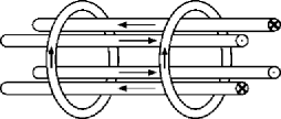
FIG. 1.: A sketch of an Ioffe trap.

The interaction potential given in Eq. 1 also causes the component of the magnetic moment perpendicular to the field to precess around the local direction of the field with a frequency $\omega$ ($\approx 180$ MHz at 1 T). If this precession is considerably faster than the change in the direction of the field seen by the neutron, that is if

$$\omega=\frac{2\mu_{n}B}{\hbar}\gg\frac{d\vec{B}/dt}{|\vec{B}|},$$ (2)

then the neutron spin will remain aligned with $\vec{B}$ as it moves throughout the trap (i.e. the neutron spin state will not change relative to the field). Under these conditions, one can essentially view the magnetic potential, $H=|\mu_{n}||B|$, as depending only on the magnitude, not the direction, of the magnetic field. Near regions in which the field approaches zero this condition is not fulfilled and trapped, low-field-seeking neutrons can invert their spin and be lost from the trap (Majorana spin-flip losses). Provided $|\vec{B}|$ is sufficiently large (i.e. no zero-field regions) a neutron initially in the trapped state will remain in the trapped state as it moves throughout the trap.

B Superthermal Production of UCN

To load neutrons into the trap their energy must be dissipated inside the trapping region. The “superthermal” process (so called because it allows one to achieve phase space densities greater than that coming from a “thermal” liquid hydrogen or deuterium cold source) is an efficient method to load the trap[21, 22].

The superthermal production of UCN in superfluid helium depends critically on the fact that cold neutrons cannot scatter with individual helium atoms as they would in a gas, but must scatter with excitations (phonons and rotons) in the superfluid. The dispersion curve (energy versus momentum) for these excitations in superfluid helium[23] is shown in Fig. 2 with the energy of the free neutron ($p^{2}/2m$) overlaid for comparison. For a neutron to scatter to the vicinity of $q=0$ via the dominant single phonon scattering process, momentum and energy conservation limit the initial neutron momentum to values of $q\sim q^{*}$. This results in the creation of a single 12 K phonon in the helium. Similarly, a UCN with $E\sim 1$ mK can only “upscatter” by absorbing a 12 K phonon (ignoring multi-phonon processes for the moment). This fact allows one to treat the neutron interaction with the superfluid as a two level system with a 12 K energy difference between the two levels.

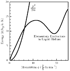
FIG. 2.: The dispersion curve for excitations in superfluid helium and the free energy of the neutron[23]. The two curves cross at $q=0$ and at $q=q^{*}$, which corresponds to a neutron wavelength of 0.89 nm, or an energy of 12 K.

The one-phonon upscattering rate can be expressed as

$$\sigma(E_{\scriptscriptstyle UCN}\rightarrow E_{\scriptscriptstyle UCN}+\Delta) =$$ (4)

$$\frac{E_{\scriptscriptstyle UCN}+\Delta}{E_{\scriptscriptstyle UCN}}\/\exp(-\frac{\Delta}{k_{B}T})\sigma(E_{\scriptscriptstyle UCN}+\Delta\rightarrow E_{\scriptscriptstyle UCN})$$

where $k_{B}$ is the Boltzmann constant. For a fixed $\Delta$ (12 K in our case), the upscattering rate can be made arbitrarily small since it decreases exponentially with the temperature $T$ of the helium bath. Physically this corresponds to decreasing the population of phonons of energy $\Delta$. In practice, however, the rates of other (multi-phonon) scattering processes dominate the upscattering rate at low temperatures. The second-order process is denoted as two-phonon upscattering, although it applies equally to the scattering of a neutron by a single phonon, in which the phonon is not absorbed. The rate of the two-phonon upscattering scales as $T^{7}$[24] and has been measured down to 500 mK [25]. In a helium bath at a temperature of 1.16 K, the upscattering rate was $2.5\times 10^{-2}$ s^-1, corresponding to a storage time of 40 s. At our operating temperature of 250 mK, the upscattering rate should be 2000 times less than the beta-decay rate. Minor modifications to the apparatus now allow the helium to be cooled below 100 mK, making the two-phonon upscattering rate negligible in performing a lifetime measurement.

The use of superfluid helium to produce UCN has been demonstrated in several previous experiments[25, 26, 27, 28] and upscattering rates have been measured in Refs. [25] and [28].

C Detection of decays in the trap

When a neutron decays in the trap, the recoiling electron scatters from atomic electrons of the helium, ionizing tens of thousands of helium atoms. The electron deposits 300 keV cm^-1 in the helium with the range of a typical electron of order 1 cm[29]. The helium ions tend to form diatomic molecular ions before recombining with electrons, leading to the creation of excited-state diatomic helium molecules. These molecules are created in both singlet and triplet states.

When each helium molecule decays it emits a photon in the extreme ultraviolet (EUV; $\lambda\approx 70-90$ nm). The singlet decays give a relatively intense pulse of light in a short time; 4000 EUV photons in less than 20 ns for a typical neutron decay[29]. These singlet decays and are used to detect the neutrons decaying in the trap. The longer decay time for the triplet states renders them less useful for this purpose. The same number of photons emitted over 13 s[31] makes it impossible to distinguish the triplet events from backgrounds.

To detect the light pulse emerging from the singlet decays directly in the trap would require EUV sensitive detectors that work at low temperatures ($<250$ mK), in liquid helium, and inside an intense magnetic field (1 T). The detectors would also be exposed to the cold neutron beam, or at least to neutrons scattering in the helium, and would need to tolerate this radiation without creating backgrounds. Finally, there is limited space available inside the magnet bore. Since it is extremely difficult to satisfy these detector requirements, the scintillation light is detected indirectly.

The EUV scintillation light is converted to blue/violet light inside the apparatus using a pure hydrocarbon, 1-1-4-4 tetraphenyl 1-3 butadiene (TPB). TPB absorbs EUV light and emits light in a spectrum ranging from 400 nm to 500 nm[30]. This light can then be transported out of the trapping region and into detectors at room temperature. The detector insert is described in detail in section III.

D Experimental Method

Each experimental run consists of a loading phase in which the neutrons are loaded into the trap and an observation phase in which the trapped neutrons are detected as they decay. At the start of a run the magnetic field is on forming the magnetic trap which will confine the neutrons. The neutron beam is turned on and neutrons begin to scatter in the liquid helium, producing UCN which become confined in the trap. The UCN creation rate is proportional to the incident neutron flux and is constant during the loading phase. UCN are lost from the trap by beta decay in proportion to the number trapped. Thus, neutrons accumulate in the trap with a time constant of the neutron lifetime or approximately 15 min. In the actual experiment, the trap is loaded for 22.5 min, yielding 78 % of the trapped UCN population that could be achieved with an infinite loading time. Once the beam is turned off, the number of neutrons in the trap decreases due to beta decay. The photomultiplier tubes are turned on 10 s after the beam is turned off and neutron decays are detected for 1 h, giving a time-varying signal directly proportional to the decreasing number of neutrons in the trap. Trapped neutrons are indicated by an exponentially decaying signal consistent with the neutron beta-decay lifetime, or a more rapid decay if there are additional trap losses.

Two classes of problems could prevent observation of this signal: spurious losses (which cause the initial trapped population to be significantly lower due to losses during loading) and background events (which could give a much higher overall counting rate and obscure a trapped neutron signal). The next two subsections will treat these two issues.

E Loss Mechanisms

Known loss mechanisms include one- and two-phonon upscattering (which as discussed above is reduced by cooling the helium target), Majorana spin-flips (which are minimized by the non-zero-field character of the trap), and ³He absorption. In addition, some neutrons with energies greater than the trap depth (that is, sufficient to allow them to escape) may be confined by the field for an extended period of time but escape from the trap before they decay.

Helium has two stable isotopes, ³He and ⁴He. While ⁴He does not absorb neutrons, ³He has an extremely high absorption cross-section. For UCN contained within a bath of ⁴He with a small amount of ³He present, the absorption rate is given by:

$$\Gamma_{abs}=x_{3}\cdot n\cdot\sigma_{th}\cdot v_{300\rm K}=x_{3}\cdot 2.6\times 10^{7}~{}\mathrm{s}^{-1}$$ (5)

where $x_{3}$ is the ratio of ³He atoms to ⁴He atoms, $n$ is the density of helium nuclei, $\sigma_{th}$ is the thermal cross section for neutron capture onto ³He and $v_{300\rm K}$ is the neutron velocity at room temperature. Isotopically purified ⁴He is available with $x_{3}<5\times 10^{-16}$[32]. At this limit, the absorption rate is $1.3\times 10^{-8}\mathrm{~{}s}^{-1}$, or ten thousand times less than the beta-decay rate. This gives a negligible shift in the trap lifetime. “Reversing” this analysis allows the data presented in section IV to yield a three standard deviation upper limit on the ³He concentration of $x_{3}\leq 5\times 10^{-11}$. A more accurate, independent measurement of $x_{3}$ using accelerator mass spectroscopy is presently being pursued.

A “marginally trapped” neutron is one with an energy greater than the trap depth, but in a trajectory that keeps the neutron confined in the trapping region for a significant time. Simulations have determined that the vast majority of these neutrons will be expelled from the trap within a few seconds[33]. In addition, it has been shown through analytical calculations[34] that by lowering the magnetic field to 30 % of its original value and then raising it back up, a trapped sample is achieved that has no neutrons stored with energies above the trap depth and about one-half of the original trapped neutrons. For this demonstration of trapping, this procedure is not necessary.

F Backgrounds

Background events are any events recorded by the data acquisition system that arise from sources other than decaying neutrons. The data acquisition system records an event when coincident PMT pulses above a set charge threshold occur on the two photomultipliers observing the trapping region. Events which are coincident with the detection of light pulses from PMTs observing plastic scintillator paddles placed below the primary detection cell are vetoed.

Hence the detection system is designed to reject several expected backgrounds. Cosmic ray muons pass through materials at a rate of 1 cm^-2 min^-1[2] and penetrate any reasonable shielding. They leave an ionization trail as they pass through, depositing roughly 2 MeV g^-1cm² times the density of the material[2]. Pulses in the primary detection system due to cosmic ray muons are vetoed by the auxiliary paddles and do not produce background events.

The requirement of coincidence between two PMTs observing the trapping region suppresses background events caused by neutron induced luminescence of materials. The neutron absorbers used to shield the materials surrounding the trapping region from the neutrons (primarily hexagonal boron nitride, hBN) glow after exposure to neutrons with a magnitude decreasing slowly on a time scale comparable to an experimental run[35]. This luminescence (which was for some time the major obstacle to extracting the trapped neutron signal) was attenuated by placing graphite between the hBN and the light collection system and by replacing the collimator and beam stop with B₄C (a material which has considerably less luminescence). To suppress this background, coincident detection in two PMTs is employed. A signal is recorded when at least two photons are detected in each PMT within a 23 ns window. With this threshold, the efficiency for detecting neutron decays is 31 %.

The system is also susceptible to background events from other sources. The passage of high-energy particles through any part of the trapping region or detection system is expected to cause scintillations in the primary PMTs. Other than cosmic ray muons which are vetoed, any particle that causes a detected scintillation will produce a background event. Such particles include decay products from radioactive nuclei, either naturally occurring or created by neutron capture during the loading phase, and neutral particles (gamma rays or fast neutrons) created outside of the apparatus. Unlike muons, gamma rays and fast neutrons tend to lose a significant fraction of their energy in each scattering event and cannot be detected with veto detectors. To reduce background events from gamma rays, the apparatus is shielded with 10 cm of lead.

Backgrounds from decays of isotopes created by neutron absorption decay exponentially with their respective lifetimes. To minimize such backgrounds, the materials exposed to the neutron beam are carefully chosen such that their primary constituents have small neutron absorption cross sections (or absorb neutrons to form a stable isotope, thus giving no background).

Despite several successful methods of reducing backgrounds, a decaying signal with peak magnitude of roughly 0.2 s^-1 had to be extracted from a time-varying background signal of about 6 s^-1 initially, with a constant component of 2 s^-1 at longer times. This was accomplished by measuring the background directly, taking half of the runs with the magnetic trap initially turned off, and subtracting this background from the trapping runs.

III Experimental Apparatus

A Beam

The experiment resides at the end of cold neutron guide number six (NG-6) in the guide hall of the NIST Center for Neutron Research (NCNR)[36]. Neutrons are released from the 20 MW reactor and are moderated by D₂O surrounding the reactor core and then by a liquid hydrogen cold source operating at a temperature of 20 K. Neutrons partially thermalize with the hydrogen and exit towards the neutron guides. Some fraction of these neutrons pass into the open end of NG-6, a rectangular ⁵⁸Ni-coated guide 60 m long, 15 cm tall and 6 cm wide.

Neutrons exiting the far end of NG-6 pass through a 6 cm diameter collimating aperture ($C_{1}$) and then through filtering materials consisting of 10 cm of bismuth and 10 cm of beryllium. The single crystal bismuth attenuates the flux of gamma rays from upstream sources. The polycrystalline blocks of beryllium Bragg-reflect neutrons with wavelengths less than 0.395 nm, removing them from the beam. The neutron beam exiting the filter has a measured capture flux of $9\times 10^{8}$ n cm^-2s^-1[5].

Immediately preceding the trapping region, a second aperture ($C_{2}$) collimates the beam before it enters the trapping region. The collimators $C_{1}$ and $C_{2}$ are chosen such that any neutron passing through both collimators will be absorbed in the beamstop at the end of the trapping region unless it scatters in the helium.

The wavelength spectrum of the beam is measured in a separate experiment by the time-of-flight method. The beam is collimated to a diameter of 400 $\mu$m. A cadmium disc positioned directly behind the collimator and rotating at 67 Hz blocks the beam except when either of a pair of slits 250 $\mu$m wide passes in front of the collimator. Neutrons passing through the slit are detected using a ³He detector placed 69 cm behind the chopper. The output of the ³He detector is recorded with a multi-channel scaler, with a 5 $\mu$s bin width. The scaler is triggered using a light emitting diode (LED) and a photodiode detecting the passage of the slit approximately 180^∘ from the neutron beam. Data from the time-of-flight spectrum is shown in Fig. 3.

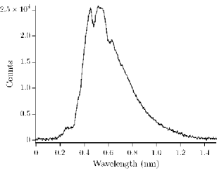
FIG. 3.: The neutron spectrum measured at the end of NG-6 using time-of-flight techniques.

Two points in the spectrum are available to set the initial time, the beryllium edge, at 0.395 nm, and the narrow slice of the beam removed by an upstream monochromator in the neutron guide at 0.48 nm. Both the unnormalized capture flux and 0.89 nm flux (important for UCN production using scattering from liquid helium) can be extracted. Using the known capture flux for normalization, the flux at 0.89 nm is

$$\frac{d\Phi}{d\lambda}=(1.62\pm 0.08)\times 10^{6}\mathrm{~{}n~{}cm^{-2}~{}s^{-1}~{}K^{-1}}.$$ (6)

The error bars are one standard deviation and primarily correspond to uncertainties in the wavelength calibration.

B Magnet

The UCN are confined in an Ioffe-type superconducting magnetic trap[19]. The magnet uses four racetrack-shaped coils to produce the quadrupole field. These consist of two different size coils and are assembled as shown in Fig. 4. The two larger coils, with 777 turns each, are 69.1 cm long by 9.2 cm high, with a coil cross-section of 3.2 cm by 2.0 cm. The smaller coils, with 336 turns each, are 65.2 cm long by 5.3 cm high, with a cross section of 1.5 cm by 2.0 cm.

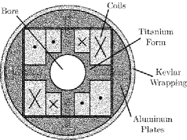
FIG. 4.: Cross-sectional view of the quadrupole magnet form.

The coils are placed onto the 6-4 ELI grade titanium form and isolated using Kapton and G-10 spacers. Aluminum compression plates, machined to give a cylindrical outer surface, are attached to the form to provide compression of the coils. This cylindrical assembly is wrapped under 67 N of tension with 20 layers of Kevlar to uniformly compress (prestress) the coils. To protect the Kevlar, the magnet was first wrapped in a layer of Tedlar then the Kevlar, and then an outer layer of fiberglass with the wrappings embedded in epoxy. The quadrupole assembly had an outer diameter of 14.5 cm and an inner bore of 5.08 cm. The ends of the titanium form were machined to mate directly with the inner vacuum can of the cryostat.

The solenoid assembly surrounds the quadrupole assembly and consists of two sets of solenoids. Each set contains a primary solenoid which is flanked by a pair of smaller solenoids with opposite polarity. These cause the magnetic field of the primary solenoid to fall off more quickly with distance along its axis. The primary solenoids each consist of 1564 turns with an inner diameter of 14.7 cm, outer diameter of 18.2 cm and length of 5.15 cm. The two “bucking” coils placed 5.0 cm on each side of the primary coil are 365 turns with an inner diameter of 14.7 cm, outer diameter of 21.5 cm and length of 1.15 cm.

The magnitude of the quadrupole field increases linearly with radius with a gradient of 0.69 T cm^-1 (at 180 A). Along the axis of the form, the field minimum (0.11 T at 180 A) is provided by the solenoids. Denoting this axis as the $z$-axis, the magnitude of the field along the $x$-axis is shown at $y=z=0$ in Fig. 5.

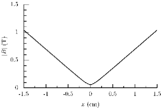
FIG. 5.: The magnetic field along the x-axis ($y=z=0$).

The solenoids each create a short high-field region closing off the ends of the trapping region. The field along the $z$-axis is shown at $x=y=0$ in Fig. 6.

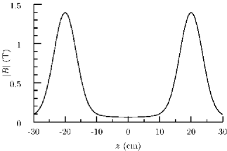
FIG. 6.: The magnetic field along the z-axis ($x=y=0$), showing the “pinch” resulting from each solenoid, closing the ends of the trap.

The depth of the magnetic trap is defined as the difference between the lowest field point at which neutrons can be lost from the trap ($B_{max}$) and the lowest field point in the trap ($B_{min}$). In our geometry, the solenoids were chosen to produce a peak field higher than the walls of the quadrupole. The trap depth is thus set by the quadrupole field at the inner edge of the detector insert (see below). This occurs at a radius of 1.59 cm, corresponding to a trapping field of 1.15 T. Subtracting the minimum field of 0.11 T gives a net trap depth of $B_{T}=1.04$ T.

C Cryogenics

Cooling the helium target below 250 mK requires the use of a ³He-⁴He dilution refrigerator which is connected to horizontally oriented magnetic trapping region. This required a custom-designed cryogenic dewar, consisting of a horizontal section to house the magnet and trapping region and a vertical section to house the refrigerator and is shown in Fig. 7.

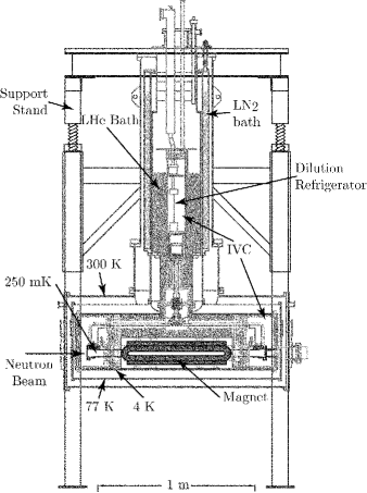
FIG. 7.: A sketch of the T-shaped dewar.

The neutron beam enters from one end of the dewar and light from the neutron decays exits from the opposite end. The neutron entrance windows consist of two layers of different materials, one to make a vacuum seal and the other to block black-body radiation, with both having good neutron transmission properties. The vacuum windows are made from a clear fluoropolymer, Teflon PFA. A simple compression seal, where the edges of a Teflon disc are compressed between two metal flanges until the Teflon begins to deform, provides the vacuum seal[37]. The windows used at 250 mK (where black-body absorbers are not needed) are 250 $\mu$m thick, 6.35 cm in diameter, leaving a 6.35 mm wide section compressed around the circumference of a window 5.08 cm in diameter. The other two windows at 300 K and 4 K are similar with a 7.62 cm diameter disc making a window 6.35 cm in diameter. To block blackbody radiation, a 50 $\mu$m thick, 6.35 cm diameter beryllium disc (Grade PF-60, Brush Wellman) covered the Teflon window at both the 4 K and 77 K end flanges. The light transmission windows, on the opposite end of the cryostat, are made from ultra-violet transmitting (UVT) acrylic (polymethyl methacrylate or PMMA) and are sealed using epoxy, indium o-ring seals, or rubber o-rings.

The isotopically pure ⁴He and detector insert are contained within the inner vacuum can (IVC) and held fixed with respect to the magnet and neutron beam, while thermally anchored to the dilution refrigerator. The helium is contained within the IVC in a tube made of 70-30 cupronickel which extends through the magnet and into the end can of the dewar. There, a copper end cap is soft-soldered (using 50/50 tin/lead solder with Nokorode paste flux) to each end of the tube to provide a sealing surface for either the Teflon window or the light transmission window. The endcaps are thermally anchored to the copper heat link which extends to the dilution refrigerator.

The cell is filled with isotopically purified ⁴He by condensing it in from room temperature. The helium is stored as a low pressure room temperature in two 450 L electropolished stainless steel tanks. The storage volume is connected to the cell through stainless steel tubing and all-metal valves. Two independent fill lines enter the dewar and each are thermally anchored at various points of the dilution refrigerator before they connect to the cell. The heat link and the fill lines are flexible near the T-section. The cell and lower half of the heat link is supported directly from the IVC using Kevlar braid.

D Neutron Shielding

When the neutron beam is open to the trapping region, $4\times 10^{8}$ n s^-1 enter the helium bath. At the end of the trapping region, those neutrons which have not scattered in the helium are absorbed in the beam dump. Since the scattering cross section for cold neutrons in liquid helium[38] decreases rapidly with wavelength, at 0.89 nm, only 6 % of the neutrons scatter, while at 0.45 nm, almost 40 % scatter. As a result, about 2$\times 10^{8}$ n s^-1 (or a total of 3$\times 10^{11}$ neutrons) scatter into the walls when the beam is on, potentially producing backgrounds.

To minimize such backgrounds, neutron absorbing materials are placed such that scattered neutrons do not reach materials that can activate. Several different materials are used, all of which contain either lithium or boron, materials which have high neutron absorption cross sections. A sketch of the shielding and windows on the beam entrance end of the dewar is shown in Fig. 8.

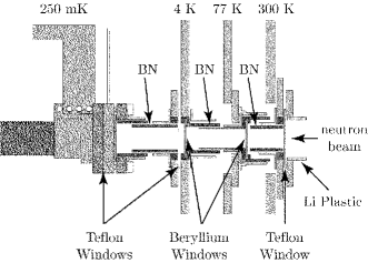
FIG. 8.: Sketch of the windows in the dewar end flanges on the beam entry end showing the interlocking boron nitride tubes shielding the beam.

The sensitivity to activation-induced backgrounds is greatest inside the detector insert and lightpipes. To minimize activation in the detection system, the materials inside the shielding are carefully chosen to contain elements which have minimal activation such as hydrogen, carbon and oxygen. Surrounding these materials is a shield of hexagonal boron nitride (hBN, grade AX05, Carborundum Corporation) to absorb the remaining neutrons. This shield consists of a series of interlocking hBN cylinders (5 cm long, with an outer diameter of 4.15 cm and a wall thickness of 1.5 mm). hBN has a neutron attenuation length of 56 $\mu$m at 0.89 nm.

The hBN is coated with a thin layer of colloidal graphite (Aerodag G, Acheson Industries) to attenuate the luminescence (see below). In addition, non-interlocking tubes of graphite (15 cm long with a wall thickness of 0.2 mm, Grade AXF-5Q1, Poco Graphite) are inserted between the boron nitride tube and detection region.

E Detection System

The detector insert is a UVT acrylic tube whose inner surface is coated with TPB-doped polystyrene (mass fraction of 40 % TPB). This insert, shown in Fig. 9, together with a series of acrylic windows and lightpipes leading to a pair of PMTs, forms a detection system allowing neutron decay events to be recorded as a function of time.

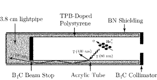
FIG. 9.: A sketch of the detector insert with the scintillation process and light transport shown (Not to scale).

Each beta-decay event in the trapping region gives rise to a pulse of EUV light in the helium. This light is downconverted to the visible by the TPB and transported past the opaque B₄C beamstop by the acrylic tube (3.8 cm outer diameter, 3.1 mm wall thickness) to a 3.8 cm diameter solid acrylic lightpipe. This lightpipe extends to the end of the helium-filled cell (see Fig. 10). At the end of the cell, the light passes through a pair of UVT acrylic windows into a 7.6 cm diameter lightpipe which extends out of the dewar. The window on the cell is formed by epoxying (Stycast 1266) an acrylic window to an acrylic tube. The other end of the tube is epoxied to an thin (0.5 mm wall thickness) aluminum cylinder (“snout”) which attaches to the cell body. The 3.8 cm lightpipe is epoxied to the window of the snout to prevent the detection insert from moving with respect to the cell. The 7.6 cm lightguide is heatsunk to the 77 K radiation shield using strips of aluminum foil as shown in the figure.

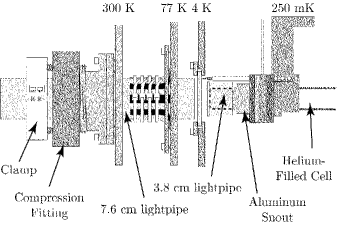
FIG. 10.: Sketch of the windows in the dewar end flanges, on the light exit end.

Outside the dewar, the light emerging from the 7.6 cm lightpipe is coupled into a pair of 5 cm diameter PMTs using a series of optical elements (Fig. 11). The light is first “condensed” as it passes through the Winston cone[39]. The light exiting the Winston cone is split into two 5 cm diameter lightpipes using a splitter which is made from two 5 cm diameter lightpipes machined at a $45^{\circ}$-angle and epoxied together, forming an ell. The corner is machined away leaving a flat elliptical surface with a 5 cm minor axis and a 7.1 cm major axis which is attached to the Winston cone. The Winston cone and the splitter are diamond turned, polished, and aluminized to maximize the light transmission. The assembly has an 80 % transmission efficiency from the 7.6 cm diameter lightpipe to the two ends of the splitter. All of the optical elements are contained within an aluminum housing which both blocks light and creates a space through which dry N₂ gas is flowed to prevent helium contamination of the PMTs.

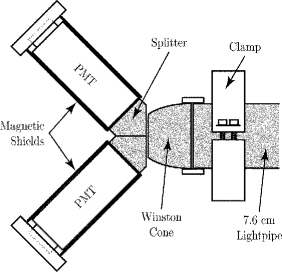
FIG. 11.: A sketch of the optical elements connecting the 7.6 cm lightpipe to the PMTs.

The photomultipliers are Burle model 8850. The signal is read out at the anode as a discrete current pulse with the tubes biased using positive high voltage.

A series of calibrations was performed using both alpha and beta sources to determine the efficiency for detecting neutron decay events. Using a ¹¹³Sn beta line conversion source ($E_{\beta}=360$ keV), the assembled detector insert and light collection system were tested using a single PMT at the end of the Winston cone. The resulting spectrum is shown in Fig. 12, with a typical pulse on average giving between 5.5 and 6.0 photoelectron signal. A series of tests using the higher energy ²¹⁰Po alpha source ($E_{\alpha}=5.3$ MeV) gives the relative detection efficiency for EUV light produced at different longitudinal positions along the cell. The efficiency varies from 75 % to 125 % (relative to the efficiency at the center of the cell) along the length and has an approximately linear dependence.

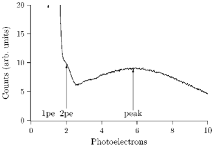
FIG. 12.: Pulse area spectrum from 360 keV beta line spectrum.

A simple Monte Carlo is used to calculate our efficiency for detecting trapped neutrons. Each event is modeled by taking a random position along the length of the cell and a random beta energy, weighted by the known shape of the beta spectrum. The results of the ¹¹³Sn calibration give an output of $14.5\pm 1.5$ photoelectrons per MeV of electron kinetic energy. The expected signal is corrected for the measured 80 % efficiency of the splitter and for the dependence of the signal on the position of the event in the cell. Requiring coincidence between pulses in both PMTs, each having an integrated area corresponding to two or more photoelectrons, results in the detection of $31~{}\%\pm 4$ % of neutron beta decays in the trapping region.

F Data Acquisition

A schematic of the data acquisition system is shown in Fig. 13. The anode signal from each of the two PMTs looking at the decay region (labeled I and J) is fanned into three outputs. One output connects directly to a digital oscilloscope, while the other two, along with the four muon veto detectors, pass into a discriminator. The voltage thresholds for the PMT signals are set to trigger on each pulse which would give a charge-integrated signal of two or more photoelectrons (denoted as I_1.5+ and J_1.5+), as determined empirically. The muons are detected using three plastic scintillators ($\rm 2.5~{}cm\times 32~{}cm\times 1.42~{}m$) which surround the lower half of the dewar and a fourth detector with slightly smaller dimensions that is placed over the PMTs and connecting lightguides. The muon thresholds are set such that each detector produces about 1000 s^-1. Varying this threshold so as to change this counting rate by more than a factor of two had no effect on the 8 s^-1 muon coincidence rate with the detector insert, indicating that all true coincidences are being included at these threshold levels.

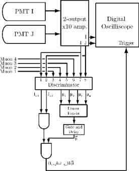
FIG. 13.: Data acquisition schematic

The outputs I_1.5+ and J_1.5+ are ANDed to produce a coincident I${}_{1.5+}\cdot$ J_1.5+ signal 23 ns long. The inverted output of the 1.5+ coincidence signal is delayed and ORed with the delayed combined muon signal to produce $\overline{(\overline{(I_{1.5+}\cdot J_{1.5+})}+\mu)}=(I_{1.5+}\cdot J_{1.5+})\cdot\overline{\mu}$, or a coincidence between I_1.5+ and J_1.5+, where no muon paddle has recorded a coincident muon. This signal is used to trigger the digital oscilloscope.

In addition to the above, the trigger output signal from the oscilloscope is recorded. This signal is used in combination with the number of times that the coincidence circuit tried to trigger the oscilloscope to correct for the deadtime of the oscilloscope and to assign time information to each scope event. The counters are active for 98 % of the time, with a dead time of 20 ms during the read out by the computer.

Digitizing the pulses with an oscilloscope allows one to integrate the area of each PMT pulse and make a cut on the integrated pulse area instead of the peak voltage. The integrated charge gives a sharper distinction between one- and two-photoelectron events, increasing the signal-to-background discrimination efficiency.

The first two input channels of the oscilloscope were connected to the amplified outputs of the two photomultiplier tubes I and J. The third, used to trigger the oscilloscope, is connected to the logic signal $(I_{1.5+}\cdot J_{1.5+})\cdot\overline{\mu}$. For each event, the oscilloscope recorded data at 250 megasamples per second for 1 $\mu$s. After 100 trigger events were recorded, the scope was read out by the computer, giving a deadtime of nearly one second between sets of 100 triggers.

IV Results

Data were taken in a series of runs, each divided into three phases (Fig. 14). For the first 100 s, the neutron beam is off. This data are used for diagnostic purposes to detect shifts in the background event rate (such as from neutron activation of materials in the trapping region with long lifetimes). In the loading phase, for the next 1350 s, the neutron beam is on and the trapped UCN population slowly increases, asymptotically approaching the theoretical maximum. During this phase the photomultiplier tubes are turned off and no events are recorded. In the last, or observation phase, data are recorded as the trapped neutron population decays for 3600 s through beta decay. Data are recorded both in the form of scaler totals each second and sets of one hundred oscilloscope events.

Two types of runs were performed. In a “trap-on” run the magnetic trap is energized throughout the entire run. In a “trap-off” run the magnet is initially off but is brought up to full current during the last 50 s of the loading phase (making conditions during the observation, phase identical between trap-on and trap-off runs). This results in a small number of trapped UCN in the trap-off runs, estimated to be at most 2 % of that in the trap-on runs. The non-trapping or trap-off data are subtracted from the trap-on data.

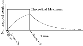
FIG. 14.: A plot of the predicted trapped neutron population over the course of a data run. Three times are indicated: the start of the run ($t=0$ s) and the times at which the neutron beam is turned on ($t=100$ s) and off ($t=1450$ s). The run ends at $t=5050$ s.

To verify that the difference in signal observed between trap-on and trap-off runs is due to the decay of trapped UCN and not from backgrounds, additional runs were necessary. Trap-on and trap-off data were taken in the same manner but with other conditions changed so that no UCN should be trapped. Specifically, data are taken with the temperature of the helium bath at 1.2 K, rather than at 250 mK (denoted as “warm runs”) and separately with the helium bath doped with enough ³He ($x_{3}=2\times 10^{-7}$) to quickly absorb trapped UCN without significantly attenuating the neutron beam (denoted as “³He runs”).

The trapping data were acquired over the course of two reactor cycles. During the first reactor cycle, from 3/23/99 to 4/5/99, a series of trapping runs was taken, followed by a set of warm runs, more trapping runs, and finally a set of ³He runs. Between reactor cycles the cell was pumped out and flushed several times with isotopically pure helium in order to cleanse the cell of residual ³He from the ³He runs. During the next reactor cycle, from 4/16/99 to 5/23/99, a longer series (about 18 days) of trapping runs was taken, followed by a series (about 20 days) of ³He runs.

In the first reactor cycle, the magnet operated at a current of 180 A, giving a trap depth of 0.75 mK. During the second cycle, a grounding problem developed in the magnet and it operated at a lower current of 120 A, resulting in a trap depth of only 0.5 mK. The number of trapped neutrons theoretically scales with magnetic field as $B^{3/2}$, resulting in the number of trapped neutrons being a factor of $\approx 0.5$ smaller than in the first cycle. The background count rate remained the same, thus even with four times as many runs, the signal extracted from the second set of data is statistically equal to that from the first set.

353 pairs (trap-on and trap-off) of data runs were taken, 87 with a trap depth of 0.75 mK and 266 with a trap depth of 0.5 mK. For the 0.75 mK set, there are 32 pairs of trapping runs, 31 pairs of warm runs, and 24 pairs of ³He runs. In the 0.5 mK set, there are 128 pairs of trapping runs and 136 pairs of ³He runs.

Data are collected using two parallel systems: storage of events using an array of scalers and digitization of the event pulses using a digital oscilloscope as discussed above. The oscilloscope data is binned into 1 s bins and is corrected for deadtime during the oscilloscope readout. This deadtime is strongly dependent on the trigger rate, which is decreasing in time over the course of a run. The exact bin in the scaler data in which the oscilloscope is being read is known. Any counts which occur in these bins are thrown out and the entire one second bin is declared as deadtime to avoid any bias. The data are then histogrammed into bins of fifty seconds where the deadtime is small and can be corrected by scaling the data by one over the live fraction. Data from the first 50 s of observation in each run contain too much deadtime to be accurately corrected in this manner and instead are removed.

The data of a given type (trapping, warm or ³He; trap-on or trap-off; 0.75 mK or 0.5 mK) are pooled together in fifty second bins and deadtime corrected. These sets of data are compared, subtracting the pooled trap-off data from the pooled trap-on data, to look for a signal (or lack thereof) indicating the decay of trapped neutrons.

The pooled data from the first reactor cycle are shown in Fig. 15. The average of the 32 trap-on runs and the 32 trap-off runs is shown starting 50 s after the beam was turned off. The difference between the two is also shown, with error bars (purely statistical uncertainty). There are several significant features in the “raw” data from the trap-on and trap-off runs. After the neutron beam has been turned off, both signals approach a level of $\sim 2$ s^-1. This component of the background is referred to as the “flat” background, since it is relatively constant over the course of a given run. At earlier times in the run, a time-varying background can be seen as well. Each of these two components of the background arises from different sources.

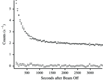
FIG. 15.: A plot of the neutron trapping data from the first reactor cycle, with the average of the pooled trap-on runs and the pooled trap-off runs shown separately. The difference is shown below, with statistical error bars.

The flat background in the earliest runs of the cycle was 1.4 s^-1, but rose quickly to 1.8 s^-1 by the second day, and averaged 2 s^-1 over the entire data set. This shift was due to the slow buildup, from neutron activation, of radioactive nuclei with lifetimes greater than one day. Approximately 0.6 s^-1 of the flat background arises from such long-lifetime activation. The remaining 1.4 s^-1 of the flat background probably arises from both gamma rays penetrating the lead shielding around the cryostat and any long-lived radioactive isotopes (such as uranium or thorium) naturally occurring in the materials of the apparatus or shielding. Without further measurements, the possibility that the majority of the present “flat” background comes from naturally occurring radioactive isotopes in our apparatus cannot be ruled out.

The time-varying component of the background could include the activation of shorter-lived isotopes, either main constituents of the apparatus or trace impurities in or near the detector. No single isotope appears to dominate this component of the background, as it did not fit well to a single exponential. Any remnant of the luminescence signal (discussed below) will also decrease with time, though this signal should be eliminated by the multiphoton threshold and requirement of coincidence between two PMTs.

Neutron absorption in the hBN (and perhaps other materials) creates color centers which relax by emitting light[35]. This luminescence signal varies with time, temperature and magnetic field, and is therefore the most problematic of our backgrounds. Cuts which were required to reduce the luminescence background also eliminate about two-thirds of the events arising from trapped neutrons. In addition, the temperature dependence of the luminescence makes the “warm” data, in which the helium was warmed to 1.2 K, potentially suspect (although unlikely to be so). Thus, because of the luminescence, data in which the helium were doped with ³He was taken to confirm the presence of trapped neutrons.

Since the luminescence most likely results from the recombination of electrons and holes in the boron nitride, it should emit single photons uncorrelated in time. Neutron decays on the other hand result in several photons being detected in coincidence between the two PMTs, providing an easy way to distinguish the neutron decay signal from the luminescence background. In practice, the rate of the luminescence signal is more than five orders of magnitude greater than the trapping signal. With a single-photon counting rate of 50,000 s^-1 in each PMT, the accidental coincidence rate (with a coincidence window of 43 ns) is 100 s^-1, three orders of magnitude larger than the expected neutron decay signal. Even the probability of three single photons arriving independently within the coincidence window is larger than the expected trapped neutron signal. The luminescence background can be reduced to a tolerable level (assuming that the luminescence photons are always uncorrelated) by requiring coincidence between four photons (corresponding to less than two false coincidences in each 1 h run). Recalling that a neutron decay in the center of the trapping region emitting a 330-keV electron will produce on average a signal of five photoelectrons, a 4 p.e. threshold is a strenuous constraint.

In practice, such a reduction in the luminescence background cannot be obtained by setting a four-photoelectron threshold on a single photomultiplier tube because there is not a sharp distinction between a three- and a four-photoelectron event. Even with a higher threshold, a single photoelectron event can result in a much larger “afterpulse” in the PMT[41, 42]. This afterpulse results from contamination of the PMT vacuum over time (especially by helium, which diffuses through glass) and occurs between 400 ns and 600 ns after the initial pulse. The size of the afterpulsing effect was studied by illuminating a PMT with light from an LED (light-emitting diode) at low current (and thus, producing predominantly uncorrelated single photons). From the pulse-height distribution, it is determined that between 2 % and 4 % of the presumably single photon pulses generated a multiple photon afterpulse. To eliminate these backgrounds, two separate photomultiplier tubes in coincidence are used, with a threshold of two photoelectrons on each.

Fig. 16 shows the pooled background subtracted data; i.e. the difference between the pooled trap-on data and the pooled trap-off data, divided by the number of runs which were pooled together. The following models are simultaneously fit to the data:

$$W_{1} = A_{1}e^{-\frac{t}{\tau}}+C_{1}$$ (7)

$$W_{2} = A_{2}e^{-\frac{t}{\tau}}+C_{2},$$ (8)

where $W$ is the experimental counting rate and the subscripts correspond to the first and second reactor cycle. The $A$’s correspond to the amplitude of the neutron decay signal, $\tau$ corresponds to the lifetime of the neutrons in the trap (assumed to be the same in each reactor cycle) and the $C$’s correspond to any residual offset between trap-on and trap-off runs, which could arise from small changes in the “flat” background rate over the course of many runs.

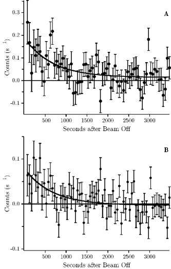
FIG. 16.: Plot of the difference between the averaged “trap-on” and the averaged “trap-off” data for reactor cycle one (A) and two (B). The solid lines indicate the result of the fits described in the text.

The data from each cycle are binned into seventy 50 s bins, with the first starting 50 s after the beam is turned off. The five parameters, $A_{1},A_{2},C_{1},C_{2},$ and $\tau$ are varied using a routine adapted from the grid fit algorithm described in ref. [43] to minimize the chi-squared ($\chi^{2}$) of the fit. The values of the fit parameters are those which yield the minimum $\chi^{2}$, and the 68 % confidence interval for each parameter is given by the range over which the $\chi^{2}$ (varying the other four parameters) increases by one relative to the minimum (varying all five parameters).

The fit gives a minimum $\chi^{2}$ of 150.67 with 135 degrees of freedom at[45]:

$$A_{1} = 0.175\mathrm{~{}s}^{-1}\pm{0.045}\mathrm{~{}s}^{-1}$$ (9)

$$A_{2} = 0.082\mathrm{~{}s}^{-1}\pm{0.021}\mathrm{~{}s}^{-1}$$ (10)

$$C_{1} = 0.014\mathrm{~{}s}^{-1}\pm{0.011}\mathrm{~{}s}^{-1}$$ (11)

$$C_{2} = -0.003\mathrm{~{}s}^{-1}\pm{0.005}\mathrm{~{}s}^{-1}$$ (12)

$$\tau = 660\mathrm{~{}s}~{}^{+290}_{-170}\mathrm{~{}s}.$$ (13)

Note that $A_{1}$ and $A_{2}$ are significantly above zero, indicating trapped UCN are present in the trap.

The data shown in Fig. 16 are evidence of an increase in the counting rate in runs in which the magnetic trap is turned on. However, from this evidence alone we cannot definitely conclude that the increase represents an additional source of counts from trapped UCN as opposed to, for example, small, magnet-dependent changes in the rate of neutron-induced backgrounds. It has been assumed that the trap-on data contain both the neutron decay signal and background events, while the trap-off data contain no decay events, but the same backgrounds. If this assumption is true, then trap-on and trap-off data taken under conditions chosen to eliminate the trapped UCN without changing the backgrounds should be consistent with each other.

To keep the background rate the same in any different experimental configuration, the detector (including the scintillation properties of the helium bath are concerned), must remain unchanged. Similarly, the neutron beam, which causes all the time-varying backgrounds, must remain unchanged as well. Two changes to the experimental configuration which meet these conditions and remove the trapped neutrons are warming the helium target to a temperature of 1.2 K and doping a small amount of ³He ($x_{3}\approx 10^{-7}$) into the isotopically purified ⁴He.

In ref. [25], the upscattering rate for UCN stored in superfluid helium was measured to be $2.5\times 10^{-2}$ s^-1 at 1.16 K, giving a UCN storage lifetime of 40 s at that temperature. During the loading phase, the continuous upscattering of UCN reduced the expected peak number of trapped UCN in our experiment from $P\tau_{\beta}$ to $P\tau_{up}$, a factor of $\tau_{up}/\tau_{\beta}\approx 0.05$. With $P=0.73$ (for the $E_{T}=0.8$ mK runs), this gives a maximum of 29 trapped UCN when the beam is turned off, or an initial beta-decay rate of 0.03 s^-1, decreasing with a lifetime of 40 s, to under 0.01 s^-1 before the first analyzed data, 50 s after the beam is turned off. This is compared to an expected rate of 0.16 s^-1 at that time in the trapping data. Since the luminescence background varies with temperature, as well as with magnetic field, the warm runs could conceivably produce a false negative. The ³He technique does not have this feature, making it a more conclusive negative than the “warm” data.

For the ³He runs, 10 Pa-L of ³He was introduced into the $8\times 10^{7}$ Pa-L of ⁴He filling the experimental cell, yielding a concentration $x_{3}\equiv n(^{3}\mbox{He})/n(^{4}\mbox{He})\approx 10^{-7}$. This concentration gives a UCN lifetime of 0.4 s and an absorption length of 400 m for 0.395 nm neutrons, the lowest wavelength neutrons passing through the beryllium filter. This attenuation is a factor of two shorter at 0.8 nm, on the tail of the spectrum. Over the 1 m length of helium in the target, the ³He should absorb less than 1 % of the beam. Thus, any background arising from the cold neutrons in the beam, rather than from UCN remaining after the beam is turned off, should be changed by less than one percent.

The data from the warm runs are shown in Fig. 17. There are no warm data from the second reactor cycle, so the data are fit only to $A_{1}$ and $C_{1}$, with $\tau=660$ s held fixed. This two parameter fit gives a result of:

$$A_{1} = 0.042\mathrm{~{}s}^{-1}\pm{0.043}\mathrm{~{}s}^{-1}$$ (14)

$$C_{1} = 0.001\mathrm{~{}s}^{-1}\pm{0.009}\mathrm{~{}s}^{-1},$$ (15)

with a $\chi^{2}$ of 76.1 for 68 degrees of freedom. This is consistent with the prediction of $A_{1}\lessapprox 0.01$ s^-1.

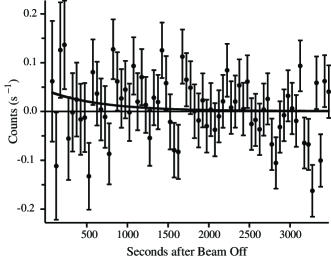
FIG. 17.: Plots of the difference between the average pooled magnetic “trap-on” and “trap-off” in the 1.2 K “warm” data taken in reactor cycle 1.

The data from the ³He runs are shown in Fig. 18. The data are fit to eq. 7 with $\tau=660$ seconds. This four parameter fit gives the following results, with a minimum $\chi^{2}$ of 119.3 for 136 degrees of freedom:

$$A_{1} = 0.045\mathrm{~{}s}^{-1}\pm{0.041}\mathrm{~{}s}^{-1}$$ (16)

$$A_{2} = -0.001\mathrm{~{}s}^{-1}\pm{0.017}\mathrm{~{}s}^{-1}$$ (17)

$$C_{1} = 0.023\mathrm{~{}s}^{-1}\pm{0.009}\mathrm{~{}s}^{-1}$$ (18)

$$C_{2} = -0.007\mathrm{~{}s}^{-1}\pm{0.0035}\mathrm{~{}s}^{-1}.$$ (19)

The amplitudes $A_{1}$ and $A_{2}$ are consistent with zero trapped UCN in the trapping region and inconsistent with the signal observed in the trapping data. The remaining constant offsets arise from the slow change in the “flat” background rate from run to run.

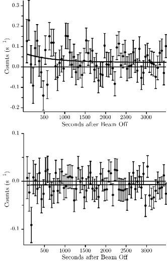
FIG. 18.: Plots of the difference between the average pooled magnetic “trap-on” and “trap-off” in the ³He data for reactor cycle one (A) and two (B).

A discussion of these results is given below.

V Discussion

For an infinite loading time, the expected initial number of trapped neutrons is given by $P\tau_{n}$, where $P$ is the production rate of trapped UCN and $\tau_{n}$ is the storage time. For a finite loading time, the initial number of trapped UCN, $N$, is given by:

$$N=P\tau_{n}(1-\exp{(-t_{\mathrm{load}}/\tau_{n})}).$$ (20)

The production rate of trapped UCN, $P$, for the 0.75 mK runs, is theoretically predicted to be $0.73~{}\mathrm{s}^{-1}\pm 0.24$ s^-1[34]. If beta decay is the only significant loss, then $\tau_{n}=\tau_{\beta}=886.7$ s[2]. Based on the predicted production rate, a loading time of $t_{\mathrm{load}}=1350$ s gives $N_{1}=500\pm 170$. In the 0.5 mK runs the production rate, $P$, and hence $N_{0}$, is scaled by a factor of (120 A/180 A)${}^{3/2}=0.544$, giving $N_{2}=270\pm 90$.

The initial count rate in our detector is given by $W=(\epsilon N)/\tau_{\beta}$, where $\epsilon=31~{}\%$ is the detector efficiency. The number of trapped neutrons observed in each data set is obtained by taking $\hat{N}_{i}=\tau_{\beta}A_{i}/\epsilon$. For the first data set, $A_{1}=0.175\pm 0.045$ gives $\hat{N}_{1}=500\pm 155$. For the second data set, $A_{2}=0.082\pm 0.021$ gives $\hat{N}_{2}=230\pm 70$. Thus, the fit to each data set is consistent with the expected number of trapped UCN. In addition, when the amplitudes of the trapping and non-trapping (“warm” and “³He) runs are combined, the trapping runs have an amplitude which is three standard deviations larger than the amplitude from the non-trapping runs. This constitutes strong evidence that we have magnetically trapped neutrons.

VI Conclusions and Future Directions

Having demonstrated magnetic trapping of UCN, we now consider the prospects for making a measurement of the neutron lifetime. First, the error bars on the measurement quoted in eq. 11 may seem discouraging, compared to the weighted world average value of $886.7\mathrm{s}\pm 1.9$ s[2]. However, the uncertainty in the present data is due entirely to statistical fluctuations in the large backgrounds being subtracted and not from the number of trapped UCNs.

There is every reason to believe that a large reduction in at least the time-varying background is possible, since these backgrounds are created by neutrons of all wavelengths, while the trapped UCN are produced by neutrons in a narrow band around 0.89 nm. Thus, a 0.89 nm nearly monochromatic beam should reduce these backgrounds by almost two orders of magnitude relative to the neutron signal.

The flat background can be reduced by increasing the detection efficiency, allowing higher rejection thresholds to be set. Presently, the efficiency is 31 %, mainly limited by the transport of the blue light down the tube surrounding the trapping region. An increase in the wall thickness of the tube will not only allow efficiencies $>90$ %, but will allow the thresholds to be raised, thereby lowering the backgrounds. The detection efficiency may also be raised by using an optically transparent beamstop rather than the opaque B₄C beamstop.

Lastly, the number of trapped UCN could be increased by building a magnetic trap either physically larger than that described here, “deeper” (in terms of magnetic trap depth), or both. The number of trapped UCN is approximately proportional to the volume of the trap ($lr_{T}^{2}$) and to $k_{T}E_{T}\propto B_{T}^{\frac{3}{2}}$. In fact, collimation constraints in setups of our type make the UCN population depend slightly more strongly on $r_{T}$ and less so on $l$. The present magnet has a bore of 5.08 cm and the diameter of the trap is 3 cm. In a larger-bore magnet, this ratio will substantially improve, giving a trap depth that is a larger fraction of the field at the bore of the magnet. An improvement of more than two orders of magnitude in the number of trapped UCN, giving a potential measurement at the 1 s level, is likely in the next few years.

Ultimately, this method of measuring the neutron lifetime is limited by losses of neutrons from the trap, which would give the appearance of a lifetime shorter than the actual beta-decay lifetime. Ways in which neutrons could be lost from the trap, other than beta-decay, include: scattering by excitations in the liquid helium, absorption by ³He, Majorana spin-flip transitions and the marginal trapping of neutrons. Scattering of trapped neutrons by excitations in the liquid helium can be reduced to below $10^{-5}$ of the beta-decay rate by cooling the helium to below 150 mK [24, 25]. Absorption by ³He is reduced by using isotopically purified ⁴He. At the level to which the supplied ⁴He has been verified[46, 47], a limit of $10^{-2}$ of the beta-decay rate can be set. The actual purity is probably better and will be measured using accelerator mass spectrometry. Majorana spin-flip transitions occur near zero-field regions and can be suppressed in an Ioffe trap by the application of a bias field. Marginally trapped neutrons can be eliminated by ramping the magnetic field down to 30% of its maximum value and then back up, resulting in a population of UCN all with energies less than the trap depth and thus all truly trapped.

The beta-decay lifetime of a neutron in a bath of liquid helium could in principle differ from that of a neutron in vacuum due to either a change in the available phase space for the decay products or a change in the matrix element that governs the decay. Small changes in the phase space factor arise from an increased or decreased amount of energy available to the decay products. For example, the minimum energy of the electron in helium is 1.3 eV[51]. The net effect of this energy difference is to increase the neutron lifetime by at most $6.5\times 10^{-6}$. We estimate that all of the phase-space effects are less than $10^{-5}$. Also, the matrix element for the decay could be influenced by the presence of the helium nuclei. The axial-vector coupling constant $g_{a}$ is known to vary by 26% compared to that of muon decay[50]. We can estimate the effect of such a change by considering the range of the strong force ($\sim 10^{-15}$ m) and the density of helium nuclei in the neutron’s environment. The effect of the helium nuclei in the environment of the neutron should be $\sim 10^{-16}$. There is no reason to expect any of these effects, or the loss mechanisms mentioned above, will prevent a measurement of the neutron lifetime at the $10^{-5}$ level, given sufficient statistics.

In addition to the immediate use of trapped UCN in a measurement of the neutron lifetime, the techniques developed for this experiment are applicable to a wide range of future experiments. The detection of EUV scintillations in liquid helium (or neon) using wavelength shifters has been proposed for use in a solar neutrino experiment[18]. Also, both the production and storage of UCN in a helium bath and the detection techniques described herein are relevant to a proposed experiment to measure the electric dipole moment (EDM) of the neutron using polarized UCN in a bath of liquid helium[17].

The apparatus described above could also be readily adapted for use as a relatively strong source of polarized UCN. This source of perfectly polarized UCN could be useful in the determination of correlation coefficients in neutron decay which can be combined with $\tau_{n}$ to test the Standard Model. A UCN beam could also be used as a probe for the investigation of condensed matter, because the UCN’s wavelength is comparable to interesting correlation lengths in crystalline, polymeric and biological materials.

REFERENCES

- [1] R.E. Lopez and M.S. Turner, Phys. Rev. D, 59, 103502 (1999).
- [2] D.E. Groom et al., Eur. Phys. J. C, 15, 1 (2000).
- [3] J. Byrne et al., Phys. Rev. Lett., 65, 289 (1990).
- [4] J. Byrne, P.G. Dawber, C.G. Habeck, S.J. Smidt, J.A. Spain, and A.P. Williams, Europhys. Lett., 33, 187 (1996).
- [5] Dr. J.S. Nico, private communication.
- [6] W. Mampe, L.N. Bondarenko, V.I. Morozov, Yu.N. Panin, and A.I. Fomin, JETP Lett., 57, 82 (1993).
- [7] V.V. Nesvizhevskiĭ, A.P. Serebrov, R.R. Tal’daev, A.G. Kharitonov, V.P. Alfimenkov, A.V. Streikov, and V.N. Shvetsov, Sov. Phys. JETP, 75, 405 (1992).
- [8] S. Arzumanov, L. Bondarenko, S. Chernyavsky, W. Drexel, A. Fomin, P. Geltenbort, V. Morozov, Yu. Panin, J. Pendlebury, and K. Schreckenbach, Nuc. Instrum. Methods, A440, 511 (2000).
- [9] V.V. Vladimirski, Sov. Phys. JETP, 12, 740 (1961).
- [10] Yu.B. Zeldovich, Sov. Phys. JETP, 9, 1389 (1959).
- [11] Yu.G. Abov, V.V. Vasil’ev, V.V. Vladimirski, and I.B. Rozhnin, JETP Lett., 44, 472 (1986).
- [12] W. Paul, F. Anton, L. Paul, S. Paul, and W. Mampe, Z. Phys. C, 45, 25 (1989).
- [13] N. Niehues, PhD thesis, Friedrich Wilhelm University of Bonn, 1983.
- [14] K.J. Kügler, K. Moritz, W. Paul, and U. Trinks, Nucl. Instrum. Methods, 228, 240 (1985).
- [15] Yu.G. Abov, S.P. Borolv, V.V. Vasil’ev, V.V. Vladimirski, and E.N. Mospan, Sov. J. Nucl. Phys., 38, 70 (1983).
- [16] J.M. Doyle and S.K. Lamoreaux, Europhys. Lett., 26, 253 (1994).
- [17] R. Golub and S.K. Lamoreaux, Phys. Rep., 237, 1 (1994).
- [18] D.N. McKinsey and J.M. Doyle, J. Low Temp. Phys., 118, 153 (2000).
- [19] Y.V. Gott, M.S. Ioffe, and V.G. Tel’kovskii, Nucl. Fusion, 3, 1045 (1962).
- [20] V.S. Bagnato, G.P. Lafyatis, A.G. Martin, E.L. Raab, and D.E. Pritchard, Phys. Rev. Lett. 58, 2194 (1987).
- [21] R. Golub and J.M. Pendlebury, Phys. Lett., A53, 133 (1975).
- [22] R. Golub and J.M. Pendlebury, Phys. Lett., A62, 337 (1977).
- [23] R.A. Cowley and A.D.B. Woods, Can. J. Phys., 49, 177 (1971).
- [24] R. Golub, Phys. Lett., A72, 387 (1979).
- [25] R. Golub, C. Jewell, P. Ageron, W. Mampe, B. Heckel, and I. Kilvington, Z. Phys. B, 51, 187 (1983).
- [26] H. Yoshiki, K. Sakai, M. Ogura, T. Kawai, Y. Masuda, T. Nakajima, T. Takayama, S. Tanaka, and A. Yamaguchi, Phys. Rev. Lett., 68, 1323 (1992).
- [27] R. Golub, D. Richardson, and S.K. Lamoreaux, Ultra-Cold Neutrons, Adam Hilger, 1991.
- [28] A.I. Kilvington, R. Golub, W. Mampe, and P. Ageron, Phys. Lett., A125, 416 (1987).
- [29] J.S. Adams, Y.H. Kim, R.E. Lanou, H.J. Maris, and G.M. Seidel, J. Low Temp. Phys., 13, 1121 (1998).
- [30] W.M. Burton and B.A. Powell, Appl. Opt., 12, 87 (1973).
- [31] D.N. McKinsey, C.R. Brome, J.S. Butterworth, S.N. Dzhosyuk, P.R. Huffman, C.E.H. Mattoni, J.M. Doyle, R. Golub, and K. Habicht, Phys. Rev. A, 59, 200 (1999).
- [32] P.V.E. McClintock, Cryogenics, 18, 201 (1978).
- [33] C.E.H. Mattoni, Undergraduate thesis, Harvard University, 1995.
- [34] C.R. Brome, Ph.D. Thesis, Harvard University, 2000.
- [35] P.R. Huffman, C.R. Brome, J.S. Butterworth, S.N. Dzhosyuk, R. Golub, S.K. Lamoreaux, C.E.H. Mattoni, D.N. McKinsey, and J.M. Doyle, J. Lumin., in press.
- [36] H. Prask, Neutron News, 5, 10 (1994).
- [37] J.S. Butterworth, C.R. Brome, P.R. Huffman, C.E.H. Mattoni, D.N. McKinsey, and J.M. Doyle, Rev. Sci. Instrum., 69, 3998 (1998).
- [38] H.S. Sommers, J.G. Dash, and L. Goldstein, Phys. Rev., 97, 855 (1955).
- [39] R. Winston, J. Opt. Soc. Am., 60, 245 (1970).
- [40] D.C.Camp, C. Gatrousis, and L.A. Maynard, Nucl. Instrum. Methods, 117, 189 (1974).
- [41] D.W. Müller, G. Best, J. Jackson, and J. Singletary, Nucleonics, 6, 53 (1952).
- [42] G.A. Morton, H.M. Smith, and R. Wasserman, IEEE Trans. Nucl. Sci., NS-14, 443 (1967).
- [43] P.R. Bevington and D.K. Robinson, Data Reduction and Error Analysis for the Physical Sciences, McGraw Hill, Inc., 1992.
- [44] P.R. Huffman et al., Nature, 403, 62 (2000).
- [45] The fit values here, and for the 3He runs differ from those cited in reference [44], because several sets of data, excluded in reference [44] are included in the fits here. The excluded data are from the first six hours of data (four runs) after any long period in which the apparatus is not irradiated. The flat background is changing rapidly between these runs, giving a non-zero and in the fits shown here.
- [46] P.C. Hendry and PVE McClintock, Cryogenics, 27, 131 (1987).
- [47] W. Henning, W. Kutschera, M. Paul, R.K. Smither, E.J. Stephenson, and J.L. Yntema, Nuc. Instrum. Methods, 184, 1247 (1981).
- [48] C.Y. Chen, Y.M. Li, K. Bailey, T.P. O’Connor, L. Young, and Z.T. Lu, Science, 286, 1139 (1999).
- [49] D.H. Wilkinson, Nucl. Phys. A377, 474 (1982).
- [50] I.S. Towner and J.C. Hardy, in Physics Beyond the Standard Model, eds. P. Herczeg, C.M. Hoffman, and H.V. Klapdor-Kleingrothaus, World Scientific, 1999.
- [51] W.T. Sommer, Phys. Rev. Lett., 12, 271 (1964).