Poster presented at the Hydrogen II workshop, Castiglione della Pescaia, June 1 –3, 2000
   
Hyperfine Structure Measurements of Antiprotonic Helium and Antihydrogen

Abstract

This paper describes measurements of the hyperfine structure of two antiprotonic atoms that are planned at the Antiproton Decelerator (AD) at CERN. The first part deals with antiprotonic helium, a three-body system of $\alpha$-particle, antiproton and electron that was previously studied at LEAR. A measurement will test existing three-body calculations and may – through comparison with these theories – determine the magnetic moment $\mu_{\overline{\mathrm{p}}}$ of the antiproton more precisely than currently available, thus providing a test of CPT invariance. The second system, antihydrogen, consisting of an antiproton and a positron, is planned to be produced at thermal energies at the AD. A measurement of the ground-state hyperfine splitting $\nu_{\mathrm{HF}}({\overline{\mathrm{H}}})$, which for hydrogen is one of the most accurately measured physical quantities, will directly yield a precise value for $\mu_{\overline{\mathrm{p}}}$, and also compare the internal structure of proton and antiproton through the contribution of the magnetic size of the $\overline{\mathrm{p}}$ to $\nu_{\mathrm{HF}}({\overline{\mathrm{H}}})$.

1 Introduction

The upcoming Antiproton Decelerator (AD) 46AD at CERN allows the formation and precision spectroscopy of antiprotonic atoms. Among the three approved experiments, the ASACUSA collaboration 46ASACUSA will as part of its program continue experiments with antiprotonic helium that were previously performed by the PS205 collaboration 46PS205 at the now closed Low Energy Antiproton Ring (LEAR) of CERN. Antiprotonic helium consisting of an alpha particle, an antiproton, and an electron (He${}^{++}-\overline{p}-e^{-}\equiv$ $\overline{\mathrm{p}}$He⁺), was found to have lifetimes in the microsecond range, thus enabling its examination with spectroscopy techniques. This unusual 3-body system has both the properties of an atom and – due to the large mass of he $\overline{\mathrm{p}}$ – a molecule and is therefore often called “atomcule”. An overview on measurements on antiprotonic helium is given in the talk by T. Yamazaki 46Yamazaki:here . The laser spectroscopy experiments of PS205 have proved that the antiproton occupies highly excited metastable states with principal and angular quantum numbers $(n,L)$ = 30$\ldots$39 (cf. Fig. 1). A major experiment at the AD will be the measurement of level splittings caused by the magnetic interaction of its constituents. Due to the large angular momentum of the antiproton, the dominant splitting comes from the interaction of the antiproton angular momentum and the electron spin. Since it is caused by the interaction of different particles, it is called a hyperfine structure (HFS). Its magnitude is about 10$\ldots$15 GHz. The antiproton spin leads to a further, by two orders of magnitude smaller splitting (called super hyperfine structure, SHFS). We describe an already installed two-laser microwave triple resonance experiment to determine this unique level splitting accurately. A measurement of the HF splitting will constitute a test of existing three-body calculations and, through comparison with these calculations, has the potential to become a CPT test by extracting a value of the antiproton magnetic moment with possibly higher accuracy than it is currently known.

The formation and spectroscopy of antihydrogen, the simplest form of neutral antimatter consisting of an antiproton and a positron, is one of the central topics at the AD. Complementary to the 1s-2s laser spectroscopy pursued by the two other experiments at the AD, ATHENA 46ATHENA and ATRAP 46ATRAP , the ASACUSA collaboration is developing a measurement of the antihydrogen ground-state hyperfine structure. This quantity is of great interest for CPT studies in the hadronic sector, since this value for hydrogen is one of the most accurately measured physical quantities, but the theoretical precision is limited by the much less accurately known electric and magnetic form factors of the proton. By measuring the HFS of antihydrogen, the value of the magnetic moment of the antiproton and its form factor, i.e. its spatial distribution, can be compared to the ones of the proton. Preliminary studies of a possible experimental layout using an atomic beam method as employed in the early stages of the hydrogen HFS measurements are presented.

2 Hyperfine Structure of $\overline{\mathrm{p}}$He⁺

Fig. 1 shows the level diagram of antiprotonic helium which was experimentally established by observing several laser-induced transitions of the antiproton (see talk by T. Yamazaki 46Yamazaki:here ). Each level in Fig. 1 is split due to the presence of three angular momenta: the orbital angular momentum $L$ (mainly carried by the $\overline{\mathrm{p}}$), and the spins of the electron $S_{e}$ and the antiproton $S_{p}$. These momenta couple according to the following scheme:

$$\vec{F} = \vec{L}+\vec{S_{e}}$$ (1)

$$\vec{j} = \vec{L}+\vec{S_{p}}$$ (2)

$$\vec{J} = \vec{F}+\vec{S_{p}}=\vec{j}+\vec{S_{e}}=\vec{L}+\vec{S_{p}}+\vec{S_{e}}$$ (3)

Due to the large orbital angular momentum of the $\overline{\mathrm{p}}$ ($L\sim 30\ldots 35$) occupying metastable states, the dominant splitting is caused by the interaction of the spin-averaged $\overline{\mathrm{p}}$ magnetic moment and the electron spin, giving rise to a doublet with $F^{+}=L+1/2$ and $F^{-}=L-1/2$ and the associated energy splitting $h\nu_{\mathrm{HF}}$ (cf. Fig. 2). This splitting is called the Hyperfine (HF) Structure. The $\overline{\mathrm{p}}$ spin causes an additional, smaller splitting for each of the HF states, which is called here the Super Hyperfine (SHF) Structure.

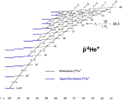
Figure 1: Energy levels of the antiproton in $\overline{\mathrm{p}}$He⁺. The $\overline{\mathrm{p}}$ is captured by replacing one of the 1s electrons, which corresponds for the $\overline{\mathrm{p}}$ to a state with principal quantum number $n_{0}\sim\sqrt{M^{*}/m}$, where $M^{*}$ is the reduced mass of the atomcule, and $m$ the electron mass. About 3% of antiprotons are captured in metastable states (black lines) at high angular momenta $L\sim n-1$, for which deexcitation by Auger transitions is much slower than radiative transitions. The lifetimes of these states is in the order of $\mu$s. The antiprotons follow predominantly cascades with constant vibration quantum number $v=n-L-1$ (black arrows) until they reach an auger-dominated short-lived state. The atomcule then ionizes within $<10$ ns and the $\overline{\mathrm{p}}$He⁺⁺  is immediately destroyed in the surrounding helium medium. The overall average lifetime of atomcules is about $3-4$ $\mu$s.

The HF and SHF structure has been calculated by Bakalov and Korobov 46Bakalov1996a ; 46Bakalov-Korobov1998 using the best three-body wavefunctions of Korobov 46Korobov1997 , and recently by Yamanaka et al. 46Yamanaka:2000 using wavefunctions calculated by Kino et al. by the coupled rearrangement-channel method 46Kino:1999 . They present the HF and SHF energies in terms of the angular momentum operators as

$$\delta E = E_{1}(\vec{L}\cdot\vec{S_{e}})+E_{2}(\vec{L}\cdot\vec{S_{p}})$$ (5)

$$+E_{3}(\vec{S_{e}}\cdot\vec{S_{p}})+E_{4}\{2L(L+1)(\vec{S_{e}}\cdot\vec{S_{p}})-6(\vec{L}\cdot\vec{S_{e}})\cdot(\vec{L}\cdot\vec{S_{p}})\}$$

The first term gives the dominant HF splitting.

The lower and the upper states of a HF doublet have $F^{+}$ and $F^{-}$, respectively. The SHF structure is a combined effect of i) (the second term) the one-body spin-orbit interaction (called historically Fine Structure, but small in the present case, because of the very large $(n,L)$), ii) (the third term) the contact term of the $\vec{S_{p}}-\vec{S_{e}}$ interaction and iii) (the fourth term) the tensor term of the $\vec{S_{p}}-\vec{S_{e}}$ interaction. According to the calculation, the contact and the tensor terms almost cancel and the SHF splitting is nearly equal to the one-body spin-orbit splitting as given by the second term. Thus, its level order (the $j^{-}=L-1/2$ level is lower than the $j^{+}=L+1/2$ level) is therefore retained.

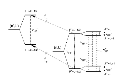
Figure 2: Laser ($f^{\pm}$), microwave ($\nu_{\mathrm{HF}}^{\pm}$), and RF ($\nu_{\mathrm{SHF}}^{\pm}$) transitions in $\overline{\mathrm{p}}$He⁺. $\nu_{\mathrm{HF}}^{*}$ is a transition between the SHF states of same total angular momentum $J=L$ that is suppressed by a factor $\sim 1/L$ compared to the allowed $\Delta L=1$ transitions $\nu_{\mathrm{HF}}^{\pm}$. The right-hand side shows the splitting of the parent state of a laser transition into a quadruplet, while on the left-hand side only the dominant doublet splitting for the daughter state is shown

2.1 Observation of a Line Splitting in a Laser Transition

According to the previous chapter, one should observe several lines in a single laser transition. Due to the large $L$, the electric dipole transitions induced by the laser pulses are subject to the selection rule $\Delta S_{e}=\Delta S_{p}=0$, which results in a quadruplet structure of each transition line, where the distance between the sub-lines is equal to the difference in splittings of the parent and daughter states. But from theoretical calculations 46Bakalov-Korobov1998 it follows that the splitting arising from the SHF structure is too small ($\approx 10\ldots 50$ MHz) to be resolved in our experimental conditions (the $\overline{\mathrm{p}}$ of momentum 100 MeV/c (5.3 MeV kinetic energy) are stopped in rather dense helium gas of temperature $\sim 6$ K and pressure $\sim 250-600$ mbar) where the Doppler broadening amounts to $\sim 400$ MHz. The splitting due to the HF coupling, however, is in the order of $1.6\ldots 1.9$ GHz for so-called “unfavoured” transitions of type $\Delta v=2$ (transitions between different cascades, see Fig. 1) which is slightly larger than the bandwidth of $\sim 1$ GHz of our laser system .

In the last beamtime at LEAR in 1996 we therefore scanned the previously discovered $(n,L)=(37,35)\rightarrow(38,34)$ transition at $\lambda=726.1$ nm by tuning our laser system to the minimum achievable bandwidth of 1.2 GHz. Fig. 3 shows the result of the high resolution scan 46Widmann1997 : a doublet structure with a separation of $\Delta\nu_{\mathrm{HF}}=1.70\pm 0.05$ GHz, in accordance with the theoretical prediction of Bakalov and Korobov of $1.77$ GHz 46Bakalov-Korobov1998 .

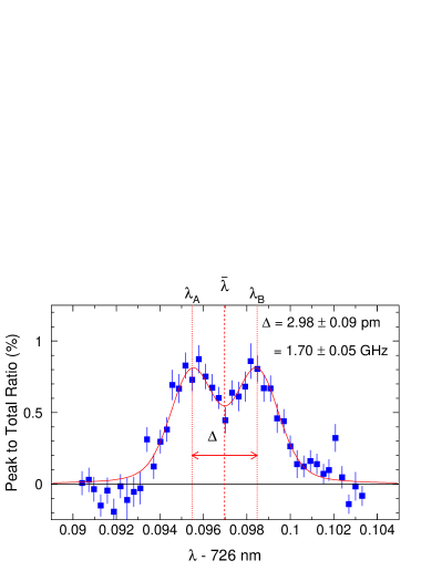
Figure 3: Observed hyperfine splitting in the $(n,L)=(37,35)\rightarrow(38,34)$ transition of antiprotonic helium. Plotted here is the area under the laser-induced annihilation peak normalized to the total delayed annihilations vs. the laser wavelength

2.2 Planned Two-Laser Microwave Triple Resonance Experiment

Due to Doppler broadening and the limited bandwidth of pulsed laser systems, the achievable accuracy in measuring the HF splitting in a laser transition is rather small. Moreover, only the difference of the splittings of parent and daughter state can be measured. A more promising way is to directly induce transitions between the HF and SHF levels within a state (e.g. the transitions labeled $\nu_{\mathrm{HF}}^{+}$ and $\nu_{\mathrm{HF}}^{-}$ in Fig. 2) by applying microwave radiation. According to 46Bakalov-Korobov1998 ; 46Yamanaka:2000 , the HF splitting for the (37,35) state amounts to $\sim 12.91$ GHz.

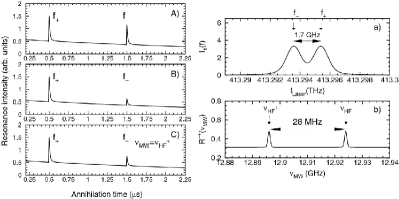
Figure 4: Two-laser microwave triple resonance experiment explained at the example of the already observed $(n,L)=(37,35)\rightarrow(38,34)$ transition. Left: Simulated delayed annihilation time spectra of the laser/microwave triple resonance method. Right: Simulated laser and microwave resonance profiles

In order to detect a microwave induced transition between the $F^{+}$ and $F^{-}$ states, first a population asymmetry has to be induced. As described in Fig. 4, this can be done by a laser pulse tuned to only the $f^{+}$ or $f^{-}$ transition. Fig. 4a) shows a resonance profile of the $(n,L)=(37,35)\rightarrow(38,34)$ laser transition assuming a realistic laser bandwidth of $\sim 0.9$ GHz, with which the doublet can be sufficiently separated. Nevertheless, a laser pulse tuned to $f^{-}$ will still partly depopulate also the $F^{+}$ states.

Fig. 4A)-C) show time spectra when two successive laser pulses are applied. In Fig. 4A), the two pulses have different frequencies, and therefore the pulse height is determined by the population of the HF levels at times $t_{1}$ and $t_{2}$ when the pulses are applied. In Fig. 4B) two pulses of the same frequency are applied. In this case the laser peak at $t_{2}$ is much smaller than the one at $t_{1}$, its height being determined by the deexcitation efficiency of the first pulse, plus feeding from upper states during the period between the two pulses.

If between $t_{1}$ and $t_{2}$ a microwave pulse is applied on resonance with one for the possible transitions between the $F^{+}$ and $F^{-}$ states (e.g. $\nu_{\mathrm{HF}}^{+}$, see Fig. 2), the population of these levels can be equalized, and the second laser pulse at $t_{2}$ will detect a larger population and thus the peak at $t_{2}$ will be larger. If the ratio $R^{++}$ of the peak areas at $t_{2}$ and $t_{1}$ is plotted against the microwave frequency, two resonances should be observed for the two allowed transitions $\nu_{\mathrm{HF}}^{+}$ and $\nu_{\mathrm{HF}}^{-}$, as shown in Fig. 4C), with the center at 12.91 GHz and a splitting of $\nu_{\mathrm{SHF}}^{+}-\nu_{\mathrm{SHF}}^{-}=28$ MHz as predicted by 46Bakalov-Korobov1998 ; 46Yamanaka:2000 .

In this way, the HF splitting of $\overline{\mathrm{p}}$He⁺ atomcules can be determined. The ultimate precision is limited by the natural width of the metastable states ($\sim 0.2$ MHz) There might, however, be distortions of the resonance line due to influences of collisions with the surrounding medium that have so far only been roughly estimated theoretically to yield only a negligible shift and a broadening of $\sim 10$ MHz 46Korenman:1999 . In this case the line center could be measured to $\sim 100$ kHz corresponding to $\sim 10$ ppm. The accuracy of the theoretical predictions are $10^{-4}$ (100 ppm) 46Bakalov-Korobov1998 and 50 ppm 46Yamanaka:2000 , and agree within 200 ppm ($2\times 10^{-4}$). The measurement will therefore test the three-body calculations and QED corrections to this accuracy.

The SHF frequencies provide information on the one-body spin-orbit and spin-spin terms. If a doublet structure with a small splitting is indeed observed in the two-laser microwave triple resonance experiment, it confirms the cancellation of the scalar and tensor spin-spin terms as predicted by theory. The observed difference of $\nu_{\mathrm{SHF}}^{+}-\nu_{\mathrm{SHF}}^{-}$ is then rather insensitive to the magnetic moment $\mu_{\overline{p}}$ of the antiproton. An observation of the suppressed transition $\nu_{\mathrm{SHF}}^{*}$ (see fig. 2) or a direct measurement of $\nu_{\mathrm{SHF}}^{+}$ or $\nu_{\mathrm{SHF}}^{-}$, however, could reveal information on $\mu_{\overline{p}}$ which is so far only known to $3\times 10^{-3}$ from X-ray measurements of antiprotonic Pb 46Kreissl .

3 Ground-State Hyperfine Structure of Antihydrogen

3.1 General Remarks

The production and spectroscopy of antihydrogen ($\overline{\mathrm{p}}$–e${}^{+}\equiv$ $\overline{\mathrm{H}}$) is one of the central topics at the Antiproton Decelerator (AD) of CERN. The two other approved experiments, ATHENA 46ATHENA and ATRAP 46ATRAP are dedicated to antihydrogen studies, and plan to precisely measure the optical 1s–2s transition in $\overline{\mathrm{H}}$ using Doppler-free two-photon spectroscopy. Tests of CPT symmetry performed by comparing hydrogen and antihydrogen can yield unprecedented accuracy since the ground state of antihydrogen has in principle an infinite lifetime, if the $\overline{\mathrm{H}}$ can be separated from ordinary matter. Those experiments therefore plan to capture the antihydrogen atoms in neutral atom trap as it has been done for hydrogen by the group of D. Kleppner 46Kleppner:here ; 46Cesar:1996 . Since the 2s state has a natural linewidth of 1.3 Hz, they hope to reach an ultimate relative precision of $1\times 10^{-18}$.

The 1s-2s transition energy is primarily due to the (electron) Rydberg constant, where the antiproton mass contributes via the reduced mass only of the order of $10^{-3}$. For the theoretical calculations an uncertainty exists at the level of $5\times 10^{-12}$ 46Sapirstein (finite size corrections) due to the experimental error in the determination of the proton radius, even if only the more reliable Mainz value of $\sqrt{<r_{p}^{2}>}=0.862\pm 0.012$ fm 46chargeradius is used (for a detailed discussion of the proton radius and its implications of precision spectroscopy in hydrogen see 46Karshenboim:pradius ). It should be noted that the recent determination of the hydrogen ground-state Lamb shift from the 1s–2s transition energy 46Udem:97 favour an even slightly larger value of the proton radius than stated above. In this sense the hydrogen and antihydrogen 1s-2s energies yield primarily information on the proton and antiproton charge distributions, respectively, once the experimental accuracy exceeds the level of $5\times 10^{-12}$.

The hyperfine structure of the ground state of the hydrogen atom is also among the best known quantities in physics, which has had a large impact on quantum physics at every stage of its development, as described in a review by Ramsey 46Ramsey . The first measurements were done 60 years 46Rabi ago with Stern-Gerlach type inhomogeneous magnets where the hydrogen atoms were deflected by the force of the magnetic field gradients onto the magnetic moment of the electron.

With the advent of the magnetic resonance method the hyperfine splitting of the hydrogen ground state was successfully determined from microwave resonance transitions by Nafe and Nelson 46Nafe and later by Prodell and Kusch 46Prodel . The precision attained by the first resonance experiment was already impressively high: $\nu_{\mathrm{HF}}({\overline{\mathrm{H}}})$ $=1420.410\pm 0.002$ MHz, which supersedes the uncertainty in the theoretical prediction of the present day, as shown below. In the early stages, room temperature hydrogen atoms were transported through inhomogeneous magnetic field and the transit time in the resonance cavity set an intrinsic limit on the resonance width. As hydrogen atoms became confined, the precision increased accordingly, and even a maser oscillation was finally observed 46Goldenberg60 . The best value to the present 46Ramsey ; 46Essen:71 ; 46Hellwig:70 is

$$\nu_{\mathrm{HF}}(\overline{\mathrm{H}})=1~{}420~{}405~{}751.7667\pm 0.0009~{}{\rm Hz}.$$ (6)

In the case of antihydrogen we can trace a similar historical development, starting from a Stern-Gerlach type experiment and proceeding to microwave resonance experiments. At each stage a meaningful value of the antihydrogen hyperfine structure constant can be obtained. The possible results and the achievable precision are discussed in the next section. Section 3.3 describes a possible experimental scenario to measure $\nu_{\mathrm{HF}}({\overline{\mathrm{H}}})$.

3.2 Hydrogen Hyperfine Structure and Related CPT Invariant Quantities

The hyperfine coupling frequency in the hydrogen ground state is given to the leading term by the Fermi contact interaction, yielding

$$\nu_{\mathrm{F}}=\frac{16}{3}(\frac{M_{p}}{M_{p}+m_{e}})^{3}\frac{m_{e}}{M_{p}}\frac{\mu_{p}}{\mu_{N}}\alpha^{2}cRy\\ ,$$ (7)

which is a direct product of the electron magnetic moment and the anomalous proton magnetic moment (here $\hbar=c=1$). Using the known proton magnetic moment, this formula yields $\nu_{\mathrm{F}}=1418.83$ MHz, which is significantly different from the experimental value and subsequently led to the discovery of the anomalous electron $g$-factor.

Even after higher-order QED corrections 46Sapirstein still a significant difference between theory and experiment remained, as

$$\delta({\rm QED})=\frac{\nu({\rm QED})-\nu({\rm Exp})}{\nu({\rm Exp})}=32.55(10)~{}{\rm ppm}.$$ (8)

This discrepancy was largely accounted for by the non-relativistic magnetic size correction (Zemach correction) 46Sapirstein :

$$\Delta\nu({\rm Zemach})=\nu_{\mathrm{F}}\frac{2Z\alpha m_{\mathrm{e}}}{\pi^{2}}\int{\frac{d^{3}p}{p^{4}}\left[\frac{G_{E}(p^{2})G_{M}(p^{2})}{1+\kappa}-1\right]},$$ (9)

where $\nu_{\mathrm{F}}$ is the Fermi contact term defined in (7), $G_{E}(p^{2})$ and $G_{M}(p^{2})$ are the electric and magnetic form factor of the proton, and $\kappa$ its anomalous magnetic moment. The Zemach corrections therefore contain both the magnetic and charge distribution of the proton.

A detailed treatment of the Zemach corrections can be found in 46Karshenboim:Zemach . Assuming the validity of the dipole approximation, the two form factors can be correlated

$$G_{E}(p^{2})=\frac{G_{M}(p^{2})}{1+\kappa}=\left(\frac{\Lambda^{2}}{\Lambda^{2}+p^{2}}\right)^{2}$$ (10)

where the $\Lambda$ is related to the proton charge radius by $r_{p}=\sqrt{12}/\Lambda$. Whether the dipole approximation is indeed a good approximation, however, is not really clear. Integration by separation of low and high-momentum regions with various separation values, and the use of different values for $r_{p}$ gives a value for the Zemach corrections of $\Delta\nu(\mathrm{Zemach})=-41.07(75)$ ppm 46Karshenboim:Zemach . With this correction, and some more recently calculated ones, the theoretical value deviates from the experimental one by 46Karshenboim:Zemach

$$\frac{\nu(\mathrm{exp})-\nu(\mathrm{th})}{\nu(\mathrm{exp})}=3.5\pm 0.9\;\mathrm{ppm}.$$ (11)

A further structure effect, the proton polarizability, is only estimated to be $<4$ ppm 46Karshenboim:Zemach , of the same order than the value above. The “agreement” between theory and experiment is therefore only valid on a level of $\sim 4$ ppm. Thus, we can say that the uncertainty in the hyperfine structure reflects dominantly the electric and magnetic distribution of the proton, which is related to the origin of the proton anomalous moment, being a current topics of particle-nuclear physics.

The hyperfine structure of antihydrogen gives unique information, which is qualitatively different from those from the binding energies of antihydrogen. As the hyperfine coupling constants of hydrogen and deuterium provided surprisingly anomalous values of the proton and deuteron magnetic moments in the history of physics, the measurement of antihydrogen hyperfine structure will, first of all, give a value of the antiproton magnetic moment ($\mu_{\overline{p}}$), which is poorly known to date (0.3 % relative accuracy) from the fine structure of a heavy antiprotonic atoms 46Kreissl . Furthermore, a precise value of $\nu_{\mathrm{HF}}(\overline{\mathrm{H}})$ will yield information on the magnetic and charge radius of antiproton.

3.3 Proposed Experimental Scenario to Measure the Ground-state Hyperfine Structure of Antihydrogen

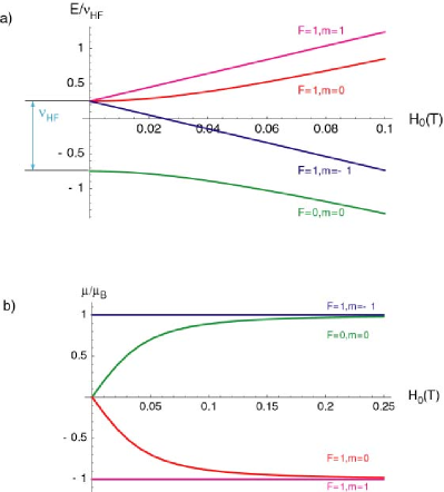
Figure 5: a) Breit-Rabi diagram of the hydrogen ground state in a magnetic field. b) dependence of the magnetic moment of he four states on the magnetic field

First it is important to remember the basics of the ground state of hydrogen in a magnetic field. The two spin 1/2 particles proton and electron (or antiproton and positron) can combine to states according to $\vec{F}=\vec{S_{\mathrm{p}}}+\vec{S_{\mathrm{e}}}$ with total spin $F$ = 0 or 1. The $F=1$ state has three possible projections to a magnetic field axis described by the quantum number $M_{F}=1,0,-1$. At zero external field these three states are degenerate, but at non-zero magnetic field their energy evolves according to the well-known Breit-Rabi diagram Fig. 5a). The two states $(F,M_{F})=(0,0)$ and $(1,0)$ have no resulting magnetic moment at zero external field, but develop one with increasing magnetic field due to the decoupling of the two spins (Fig. 5b).

In the following the different steps of the experiment are described.

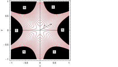
Figure 6: Cross section of a sextupole magnet with magnetic field lines (red). The direction of the atoms is perpendicular to the cross section

Antihydrogen Formation

The first step towards a measurement of $\nu_{\mathrm{HF}}({\overline{\mathrm{H}}})$ is the formation of Antihydrogen. Here we assume the formation scheme and parameters of the ATHENA 46ATHENA-form experiment at CERN/AD.

• $\overline{\mathrm{H}}$ is formed form clouds of antiprotons and positrons trapped in Penning traps.

• the formation will be done by pushing antiprotons through a rotating positron plasma. The rotation is an unavoidable result of the $\vec{E}\times\vec{B}$ drift of the positrons in the magnetic field. The rotation frequency depends on the spatial density of the plasma 46plasmarot .

• the antiprotons will stop in the e⁺-plasma and begin thermal diffusion until they form $\overline{\mathrm{H}}$.

• the $\overline{\mathrm{H}}$ atoms will not be confined by the constant solenoid field and therefore leave the trap region with an energy distribution given by the temperature of the e⁺-plasma and its rotation speed.

Transport and Spin Selection by Inhomogeneous Magnetic Fields

Since the $\overline{\mathrm{H}}$ atoms will leave the solenoid not as a collimated beam, it is straight forward to use sextupole magnets to focus them as it was commonly done it atomic beam experiments 46atombeam . The sextupole magnet will at the same time act as a filter to select one of the two hyperfine states. This can bee seen from writing the potential energy $V$ of a magnetic moment of a spin-1/2 particle in a magnetic field and the resulting force $K$:

$$V = -\vec{\mu}\cdot\vec{H(\vec{x})}$$ (12)

$$\vec{K} = -\nabla V=\pm\mu\;\nabla H,$$ (13)

where the sign of $K$ depends on whether $\vec{\mu}$ and $\vec{H}$ are parallel or antiparallel. From Fig. 5b) it is clear that the states $(F,M_{F})=(1,1)$ and $(1,0)$ prefer lower magnetic fields since this minimizes their energy (“low-field seekers”), while the opposite is true for the other two states.

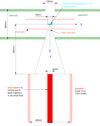
Figure 7: Layout of the split solenoid magnet for antihydrogen production and extraction

For a sextupole, the magnetic field is proportional to the square of the radius, and the force therefore becomes proportional to $r$ (cf. Fig. 6):

$$H_{\mathrm{sextupole}}=\frac{C}{2}\,r^{2}\rightarrow K_{\mathrm{sextupole}}=\pm C\mu r.$$ (14)

For the (1,1) and (1,0) states this force points towards the center of the sextupole and acts like the restoring force of a harmonic oscillator for atoms leaving the center line. This leads to a harmonic oscillation in $r$, perpendicular to the propagation direction. Atoms with the same velocity will therefore undergo point-to-point focusing, where the focal length depends on the velocity.

Fig. 7 shows a realistic layout of a Penning trap in a split solenoid magnet, where a sextupole magnet is placed under 90 degrees to the solenoid magnetic field axis. The splitting of the solenoid as well as a split electrode or one made out of a mesh are necessary to let the $\overline{\mathrm{H}}$ atoms pass without destroying them.

The further layout of the experiment consists of a first sextupole S1 as a spin selector, a microwave cavity, and a second sextupole S2 as a spin analyzer (cf. Fig. 8). Since the magnetic field in S1 is higher on the outside, the “low-field seekers” (1,1) and (1,0) will be focused, while the “high-field seekers” will move towards the magnet poles and annihilate there. We further assume that the states with $M_{F}=0$ that have no permanent magnetic moment will loose their orientation in the field-free region before S1, so that after S1 only atoms in the state (1,1) will remain.

Microwave Induced Spin-Flip Transition and Detection

A microwave cavity placed between S1 and S2 can induce spin-flip transitions $(F,M_{F})=(1,1)\rightarrow(1,-1)$ if tuned to $\nu_{\mathrm{HF}}({\overline{\mathrm{H}}})$. In order to produce a positive signal, i.e. an increase in counting rate after S2 under resonance condition, S2 will be rotated by 180 degrees with respect to S1. Therefore, the $(1,-1)$ state where $M_{F}=-1$ is defined with respect to the magnetic field direction in S1 will be a (1,1) state in S2, while the (1,1) state of S1 without spin flip would correspond to a $(1,-1)$ state in S2. As a result, if the microwave frequency is off resonance, no $\overline{\mathrm{H}}$ atoms will reach behind S2, while on resonance an increase in the number of atoms should be detected after S2.

Table 1: List of parameter used in the simulation of $\overline{\mathrm{H}}$ trajectories

Source parameters	value	comment
internal temperature of particle clouds	10 K
rotation frequency of e+ plasma	100 kHz	for $10^{8}$ e+/cm3
diameter of e+ plasma	2 mm	FWHM gaussian
length of e+ plasma	5 cm
Sextupole parameters
max. field at pole	1 T
outer diameter sextupole	40 cm
inner diameter sextupole	5 cm	blocked to reduce background
		of $\overline{\mathrm{H}}$ atoms hitting directly
		the counter
Microwave cavity
typical dimensions	21 cm	wavelength for $\nu=1.4$ Ghz

The achievable resolution for $\nu_{\mathrm{HF}}({\overline{\mathrm{H}}})$ in this type of experiment is determined by the flight-time of the atoms through the cavity. Taking the average velocity of the atoms of 650 m/s (determined by the assumptions given in Table 1) and a typical cavity length of 10 cm, a width of the resonance line of $\sim 7$ kHz results corresponding to a fraction of $5\times 10^{-6}$ relative to $\nu_{\mathrm{HF}}({\overline{\mathrm{H}}})$ = 1.4 GHz. Using a cavity of 50 cm length the width of the resonance line will be reduced to 1 ppm. With enough statistics the center of the line can be determined to about 1/100 yielding an ultimate precision of $\sim 10^{-8}$.

Monte-Carlo Simulation of Proposed Experiment

In order to estimate the efficiency of the setup as described above, a Monte Carlo simulation was performed for the whole experiment by numerically integrating the equation of motion

$$\vec{K}=m\frac{\mathrm{d}^{2}\vec{x}}{\mathrm{d}t}=-\mu_{\mathrm{eff}}(H(\vec{x}))\frac{\mathrm{d}H(\vec{x})}{\mathrm{d}\vec{x}},$$ (15)

with $\vec{x}=(x,y,z)$ being the position of the atoms.

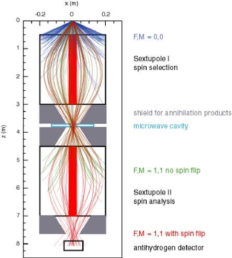
Figure 8: Trajectories of antihydrogen atoms through two sextupole magnets as calculated by a Monte-Carlo method. Please not the the X and Z axis do not have he same scale

The magnetic field of the split solenoid was calculated by numerically solving the Biot-Savart law for the geometry as described in Fig. 7 and a field of about 3 T at the center. Inside the sextupole magnet the magnetic field was calculated according to the analytical formula $H(r)\propto r^{2}$ with $r^{2}=x^{2}+y^{2}$, assuming a maximum field of $H(r_{\mathrm{max}})=1$ Tesla ($r_{\mathrm{max}}$ being the radius of the sextupole magnets). The main assumptions are summarized in Table 1.

Typical trajectories calculated by this Monte Carlo method are shown in Fig. 8. The overall result is that about $7\times 10^{-5}$ of all antihydrogen atoms initially formed in the trap region can be transported to the $\overline{\mathrm{H}}$ detector after S2. At expected formation rates of about 200/s 46ATHENA-form this would result in a count rate of 1 event per 2 minutes on resonance. This seems rather small, but is feasible since the antihydrogen atoms can be easily detected with unity efficiency from the annihilation of their constituents.

4 Conclusion and Summary

The experiments with antiprotonic atoms discussed in this paper have different main topics. The measurement of the hyperfine structure of antiprotonic helium, which is already in progress at the AD at CERN, will primarily test the accuracy of 3-body calculations in the extreme situation of one particle having an angular momentum quantum number of $\sim 35$. This makes it a very difficult and challenging problem to few-body theory. If the experimental accuracy could become high enough, we would be able to perform a test of CPT theory for the magnetic moment of proton and antiproton by comparing the experimental result to the calculations that use the much better known value of the magnetic moment of the proton. The equality of proton and antiproton magnetic moment is experimentally only know to an accuracy of 0.3%.

A measurement of the ground-state hyperfine structure of antihydrogen would primarily be a CPT test in the hadronic sector, since the leading term is directly proportional to the magnetic moment of the antiproton. It is therefore a complementary measurement to the proposed 1s-2s spectroscopy of antihydrogen, since the optical spectrum of antihydrogen is dominated by the positron mass. The experimental value for the hyperfine structure of hydrogen has for 30 years been one of the most precisely measured value in physics (uncertainty $<10^{-12}$) and has only recently been surpassed by the 1s-2s two-photon laser spectroscopy. On the other hand there exists an uncertainty in the theoretical calculations on the level of $\sim 4$ ppm due to the finite size of the proton, i.e. its electric and magnetic structure and polarizability. A determination of the hyperfine splitting of antihydrogen with higher precision will therefore give insight into the internal structure of the antiproton in comparison to the proton, which is an actual topic in nuclear and high energy physics in relation to the origin of the anomalous magnetic moment of the proton. The experiment sketched in this paper seems feasible provided the assumptions on the circumstances of antihydrogen production are reasonable. More will be known about these when the first cold antihydrogen atoms will be produced at the AD, hopefully this year or in the year 2001. With enough statistics a resolution well below the ppm level can be easily reached for the hyperfine splitting and therefore the antiproton magnetic moment.

References

-
(1)
AD homepage:
http://www.cern.ch.PSdoc/acc/ad/ -
(2)
T. Azuma et al: CERN/SPSC 97-19, CERN/SPSC
2000-04; ASACUSA home page
http://www.cern.ch/ASACUSA/ -
(3)
PS205 home page:
http://www.cern.ch/LEAR_PS205/ - (4) T. Yamazaki: this edition
- (5) C. Amsler et al.: this edition, pp. 449–468
- (6) J. Walz et al.: this edition, pp. 501–507
- (7) D.D. Bakalov et al.: Phys. Lett. A 211, 223 (1996)
- (8) D.D. Bakalov and V.I. Korobov: Phys. Rev. A 57, 1662 (1998)
- (9) V.I. Korobov and D.D. Bakalov: Phys. Rev. Lett. 79, 3379 (1997)
- (10) N. Yamanaka, Y. Kino, M. Kamimura, and H. Kudo: Phys. Rev. A, in print
- (11) Y. Kino, M. Kamimura, and H. Kudo: Hyperfine Interaction 119, 201 (1999)
- (12) E. Widmann at al.: Phys. Lett. B 404, 15 (1997)
- (13) G. Korenman: private communication (1999)
- (14) A. Kreissl et al.: Z. Phys. C 37, 557 (1988)
- (15) D. Kleppner: this edition, pp. 29–43
- (16) C. Cesar et al.: Phys. Rev. Lett. 77, 255 (1996)
- (17) J.R. Sapirstein and D. R. Yennie: ‘Theory of Hydrogenic Bound States’. In: Quantum Electrodynamics, ed. by T. Kinoshita (World Scientific, Singapore 1990) pp. 560–672
- (18) G.G. Simon, Ch. Schmitt, F. Borokowski and V.H. Walther: Nucl. Phys. A 333, 381 (1980)
- (19) S. G. Karshenboim: Can. J. Phys. 77, 241 (1999)
- (20) Th. Udem et al.: Phys. Rev. Lett. 79, 2646 (1997)
- (21) N. Ramsey: ‘Atomic Hydrogen Hyperfine Structure Experiments’. In: Quantum Electrodynamics, ed. by T. Kinoshita (World Scientific, Singapore 1990) pp. 673–695
- (22) I.I. Rabi, J.M.B. Kellogg and J.R. Zacharias: Phys. Rev. 46, 157 and 163 (1934); J.M.B. Kellogg, I.I. Rabi and J.R. Zacharias: Phys. Rev. 50, 472 (1936)
- (23) J.E. Nafe and E.B. Nelson: Phys. Rev. 73, 718 (1948)
- (24) A.G. Prodell and P. Kusch: Phys. Rev. 88, 184 (1952)
- (25) H.M. Goldenberg, D. Kleppner and N.F. Ramsey: Phys. Rev. Lett. 8, 361 (1960)
- (26) L. Essen, R.W. Donaldson, M.J. Bangham and E.G. Hope: Nature 229, 110 (1971)
- (27) H. Hellwig et al.: Proc. IEEE Trans. IM-19, 200 (1970)
- (28) S. G. Karshenboim: Phys. Lett A 225, 97 (1997)
- (29) M. Niering et al.: Phys. Rev. Lett. 84, (2000)
- (30) S.R. Lundeen and F.M. Pipkin: Phys. Rev. Lett. 46, 232 (1981)
- (31) D.E. Groom et al.: Europ. Phys. J. C 15, 1 (2000)
- (32) R. Landua, ATHENA spokesman: private communication (2000)
- (33) P. Kusch and V.W. Hughes: ‘Atomic and Molecular Beam Spectroscopy’. In: Encyclopedia of Physics Vol. XXXVII/1, ed. by S. Flügge (Springer, Berlin 1959) pp. 1–172
- (34) F. Anderegg, E.M. Hollmann, and C.F. Driscoll: Phys. Rev. Lett. 81, 4875 (1998)