Search for Strange Quark Matter Produced in Relativistic Heavy Ion Collisions

Abstract

We present the final results from Experiment 864 of a search for charged and neutral strange quark matter produced in interactions of 11.5 GeV/c per nucleon $Au$ beams with $Pt$ or $Pb$ targets. Searches were made for strange quark matter with $A\geq 5$. Approximately 30 billion 10% most central collisions were sampled and no strangelet states with $A\leq 100$ were observed. We find 90% confidence level upper limits of approximately $10^{-8}$ per central collision for both charged and neutral strangelets. These limits are for strangelets with proper lifetimes greater than 50 ns. Also limits for $H^{0}$-d and pineut production are given. The above limits are compared with the predictions of various models. The yields of light nuclei from coalescence are measured and a penalty factor for the addition of one nucleon to the coalescing nucleus is determined. This is useful in gauging the significance of our upper limits and also in planning future searches for strange quark matter.

25.75.-q

I Introduction

Color singlet states observed so far consist of three quarks (baryons), three antiquarks (antibaryons) or quark-antiquark pairs (mesons). These states are described by the Standard Model which does not forbid the existence of color singlet states in a bag containing an integer multiple of three quarks. In such quark matter states all the quarks are free within the hadron’s boundary and so are inherently different from nuclear states that are composed of a conglomerate of A = 1 baryons. Quark matter states composed of only up and down quarks are known to be less stable than normal nuclei of the same baryon number A and charge Z since nuclei do not decay into quark matter. This is because of the relatively large Fermi energy of two-flavor quark matter.

Strange quark matter (SQM), composed of strange as well as up and down quarks, has several stabilizing factors that could result in quasistable states. The presence of strange quarks lowers the Fermi energy and the most stable configurations for a given A would have roughly equal numbers of up, down and strange quarks with charges of +2/3e, -1/3e and -1/3e, respectively, therefore minimizing the surface and Coulomb energies. A major destabilizing factor is the large mass of the strange quark. The above factors imply that the most stable varieties of strange quark matter should have a low value of Z/A and increase in stability with mass number. The property of low Z/A provides the basis for current SQM searches at heavy ion accelerators.

A Theoretical predictions for strange quark matter

Chin and Kerman [20] in 1979 predicted that SQM with $A\leq 10$ might be metastable with halflife$\leq 10^{-4}s$. These predictions used quantum chromodynamics (QCD) and the MIT bag model of hadrons [21] to treat SQM quantitatively. Subsequently, similar calculations with the addition of shell effects were carried out by Farhi and Jaffe [22] and Gilson and Jaffe [23]. All theories contain the prediction that SQM systems become more stable as A increases due to the small total charge of SQM and bag model effects. For sufficiently large A ($A\sim 100$ to $A\sim 10000$, depending on the parameters assumed), SQM might be absolutely stable [24]. At the low-mass end Jaffe [25] proposed the existence of a neutral metastable dibaryon called the $H^{0}$ consisting of (uuddss) quarks. Its lifetime was estimated [26] to be less than $\sim 2\times 10^{-7}$.

It has been postulated that there may exist compact astrophysical objects composed entirely of strange matter called strange stars. Several astrophysical mechanisms are available to convert very large stars to strange stars as discussed by Li et al.[27] and references therein. They also postulate that the millisecond pulsar SAX J1808.4-3658 is a good candidate for a strange star.

For smaller A, SQM may be metastable if strong decays are forbidden, but could undergo weak decays with lifetimes in the range from $10^{-4}$ to $10^{-10}$ sec [20, 28, 29]. Effects of Pauli blocking may help to increase SQM lifetimes. Such systems with $A\leq{100}$ which might be produced in relativistic heavy ion collisions are commonly called strangelets and are predicted to be metastable for a wide range of SQM properties and bag model parameters [22, 23, 29]. Due to the lack of theoretical constraints on bag model parameters and difficulties in calculating color magnetic interactions and finite size effects [30, 31] experiments are necessary to help answer the question of the stability of strangelets if indeed they do exist.

Relativistic heavy ion collisions provide a promising mechanism for producing strangelets in the laboratory due to the high baryon densities and the large number of strange quarks achieved in a small volume during these collisions. Several classes of models have been generated to describe strangelet production in nucleus-nucleus collisions. They can be classified into two categories, namely strangelet production by coalescence or strangelet production following quark-gluon plasma (QGP) production.

In coalescence models [32] a number of A=1 particles are produced in the collision that in turn fuse to form a strangelet. Thermal models further assume that thermal and chemical equilibrium are achieved prior to the production of the final particles [33]. Coalescence and thermal models usually predict lower strangelet cross sections than models that postulate a collision in which a QGP state is formed.

It might be possible to produce a phase transition to a QGP in these collisions. Under these conditions the hot quark matter might cool into a metastable state of cold SQM resulting in a strangelet. Models have been produced to examine production of strangelets following QGP formation. Kapusta et al. estimate that at AGS energies there could be rare events in which a droplet of QGP is nucleated converting most of the superheated matter to plasma [34]. They calculate the probability that thermal fluctations in a superheated hadronic gas will produce a thermal droplet and that the droplet will be large enough to overcome its surface free energy and grow. They estimate this to occur in between 0.1% and 1% of central (small impact parameter) $Au$ + $Au$ collisions at AGS energies.

Greiner et al. suggests that once a QGP droplet is formed, for a wide range of QGP properties, almost every QGP state evolves into a strangelet by means of the strangeness distillation mechanism providing strangelets are metastable [35]. The droplet cools by emitting mesons but the $\overline{s}$ quarks preferentially joins with u and d quarks to form K mesons in the baryon rich plasma formed at AGS energies. This leaves the QGP enriched in strangeness relative to anti-strangeness leading to the formation of a strangelet during the hadronization process. This process favors the formation of the more stable large strangelets since the QGP would lose energy by meson emission possibly resulting in a strangelet of approximately the same A as the QGP droplet. It is thus important to carry out experiments that are sensitive to a large mass range.

Other estimates of strangelet production by distillation from the QGP were carried out by Liu and Shaw [36] and Crawford [37]. They predict a wide range of production levels. Strangelet production could prehaps be as high as $10^{-4}$ to $10^{-3}$ per central $Au+Au$ collision at AGS energies. Based on a recent calculation, Schaffner-Bielich et al. have suggested that at low masses negative strangelets are more likely to be formed than positive strangelets [38]. They used the MIT bag model with shell mode filling for various bag parameters. Their model also predicts a number of neutral strangelet states to be metastable.

In this experiment we have searched for positive, negative and neutral strangelets with masses up to A=100. We note that our apparatus would detect strangelets of $A\geq 100$ if they were produced. However, the production probability with coalescence would certainly vanish at baryon numbers of the order of 100 or more. The strangeness distillation model would produce strangelets which at the extreme would be less than the total numner of baryons in the collision (197+208 for a $Au-Pb$ collision). Furthermore, due to saturation in the response of the E864 calorimeter, all masses higher than A=100 would be detected as having mass very close to A=100. For these reasons we show our yields as functions of A up to A=100.

B Previous searches for strange quark matter

Searches for in situ SQM have been made on terrestrial matter [39], cosmic rays and astrophysical objects [40]. These searches resulted in extremely low limits for strangelets in terrestrial matter. These rates are less than predicted by Big Bang models of strangelet production in the early universe and so would argue against the existence of completely stable strangelets. This conclusion, however, is somewhat ambiguous due to the uncertainties in the models themselves, the uncertainty in estimating strangelet survival probabilities and possible geophysical processes which could “distill” the terrestrial strangelets into unaccessible regions.

With the advent of relativistic heavy ion beams at the AGS and SPS accelerators it is possible to search for metastable strangelets in the reaction products from central collisions where a large number of strange quarks are produced. Searches for strangelets have been carried out using relativistic heavy ion beams from the AGS and SPS accelerators. Early searches which used $Si$ + $Cu$ [41] and $Si$ + $Au$ [42] reactions at the AGS accelerator and $S$ + $W$ [43] reactions at the SPS accelerator yielded null results. Later experiments at the AGS accelerator using $Au$ beams [44] and at the SPS accelerator using $Pb$ beams [45] also yielded null results despite the increased production potential of these heavier beams. To date no experiment has published results indicating a clear positive signal for strangelets so all have set production upper limits.

The searches for strangelets discussed above using relativistic heavy ion collisions were sensitive to proper lifetimes down to about 50 ns. All of these experiments except the one carried out by E814 [41] used focusing spectrometers which, for a given magnetic field setting, have good acceptance only for a fixed momentum and charge of the produced particle. Therefore, the production limits obtained in these experiments are strongly dependent upon the production model assumed for high mass particles such as strangelets.

Recent searches for the $H^{0}$ dibaryon have been carried out. If the $H^{0}$ decays weakly by $\Delta S=+1$ then the expected lifetime is similar to that of the $\Lambda$, therefore most searches look for decay processes with $\Lambda$ type lifetimes. However, if the $H^{0}$ is very tightly bound, then only $\Delta S=+2$ decays are allowed and a resulting lifetime of the order of 50 ns is possible. Using the 1.8 GeV/c $K^{-}$ beam from the AGS, Stotzer et al.[46] in E836 searched for the $H^{0}$ at a mass range from 50 to 380 MeV/$c^{2}$ below the $\Lambda\Lambda$ threshold. E810 and E888 have also carried out searches for the $H^{0}$ dibaryon[47, 48] at the AGS by searching for it’s decay modes but conclusive evidence for it’s existence has not been obtained. The neutral beam produced by 800 GeV/c protons on a $BeO$ target was analyzed by the Fermilab KTeV collaboration[49] to search for the $H^{0}$. No events consistent with interpretation as an $H^{0}$ were observed. A complete summary of searches carried out for various forms of strange quark matter is given in a review article by Klingenberg [50].

The primary goal of the E864 experiment was to search for charged and neutral strangelets with lifetimes $\geq 5\times 10^{-8}$ seconds, baryon number A from 6 up to 100 and charge to mass ratios lower than most normal nuclei. These characteristics suggested a strategy of looking for mid-rapidity, massive objects with an unusual Z/A ratio in an apparatus with a high rate capability and redundancy for background rejection. The E864 apparatus implemented this strategy as described in the next section. E864 results from earlier data sets with smaller statistics than the results shown here have been published for charged strangelets in a series of papers by Armstrong et al. [51] as well as for neutral strangelets [52]. In this paper we give the final limits for both charged and neutral strangelets from the E864 experiment.

II The E864 Experiment

A General design of experiment

The E864 experiment is an open geometry, two dipole magnetic spectrometer designed to search for strangelets in $Au$ + $Pt,Pb$ collisions at 11.5 GeV/c per nucleon. The experiment is described in detail in Ref [53]. The open geometry with only dipole magnets causes the experiment to be less sensitive to the shape of a particle’s production differential cross section. Due to the nature of the design of the rare particle search, the spectrometer is also well suited for detecting nuclear isotopes and hypernuclei produced by coalescence following central collisions.

The spectrometer identifies particles via their mass M and charge Z. In order to conduct this search, E864 has a large geometric acceptance (5 msr) and operates at a high data rate. The emphasis is on the measurement of particles near the center-of-mass rapidity since it leads to an efficient search with minimal production model dependence. A diagram of the spectrometer is shown in Figure 1. The main components are beam defining counters, a target system (usually $Pb$ or $Pt$), a multiplicity counter for triggering on the centrality of the event, two analysis dipole magnets, three stations of hodoscopes for Time-of-Flight (TOF) and tracking, two stations of straw tubes for tracking, a hadronic calorimeter and a large vacuum tank not shown in this figure. The experiment also utilizes a high speed data acquisition system (2.7 Mbytes per second) and a flexible second level trigger (Late Energy Trigger) based on TOF and energy as measured by the calorimeter.

B Experimental details

1 Target area

The E864 spectrometer receives a fully stripped $Au$ beam with a momentum of 11.5 GeV/c per nucleon. The ions are incident on a $Pb$ or $Pt$ target of thickness between 5% and 60% of a $Au$ interaction length. The nucleon-nucleon center of mass energy is 4.6 GeV and its rapidity $y$ is 1.6. The experimental layout in the target area consists of quartz Cherenkov beam counters (MITCH) and beam defining counters and a scintillator multiplicity counter to select events with the desired centrality. Thin quartz plates are used for all counters traversed by the beam to minimize the number of interactions in the counters. The beam counters measure the incident beam flux and provide the start time for the hodoscope and calorimeter TDCs [54].

The multiplicity counter consists of a four quadrant annulus placed around the beam pipe 13 cm downstream of the target. It subtends an angular range of $16.6^{o}$ to $45.0^{o}$. The total signal measured with this counter is proportional to the centrality of the collision and is used to trigger on the centrality of the events. Most data is taken with a threshold to accept the 10% of events with the largest multiplicity counter signals.

2 Tracking systems

The heart of the spectrometer tracking is the scintillator TOF hodoscope system which consists of three stations, H1, H2 and H3, whose locations are shown in Figure 1. The hodoscopes provide redundant measurements of a particle’s TOF as well as its position. Requiring that a good space track also have consistent velocities as measured at each of the hodoscopes significantly improves the background rejection. The hodoscopes also give three independent charge measurements via the pulse height information from energy loss ($dE/dx$) in the scintillator. The hodoscopes provide $x-y-z$ space points. The time resolution for H1 and H2 is $140\pm 10$ ps and for H3 is $160\pm 10$ ps. The measured efficiencies of the hodoscopes range from 97.7% for H1 to 98.9% for H2 and H3.

In order to improve the spatial resolution for tracked particles, the spectrometer has two stations of straw tubes, referred to as S2 and S3 in Figure 1. A complete description can be found in Reference[55]. Each station consists of three sub-planes ($x,u,v$) each consisting of two layers. The straws of the x plane are mounted vertically and the straws of the u and v planes are mounted at $\pm$20^o relative to vertical, respectively. Each sub-plane consists of two staggered layers of straw tubes 4 mm in diameter. The planes are rotated around the vertical axis at approximately 6 degrees with respect to the beam line so that most particles are incident perpendicular to the planes.

A straw tube chamber S1 was placed inside the vacuum tank between M1 and M2. The chamber was designed to improve the tracking by providing a track measurement between the magnets. However, due to a problem with discharges associated with the high voltage connections, the chamber did not work well enough to be useful. Due to the exigencies of the experimental run, the chamber was left in place and contributed to background scattering processes. The analysis which we carried out is correct but would have given a slightly more sensitive result if S1 had been removed.

3 The calorimeter

The final element of the spectrometer is a “spaghetti” design hadronic calorimeter located at the end of the E864 beamline as shown in Figure 1. Its purpose is to provide a second independent mass measurement for charged particles and to identify neutral particles based on $\beta$ and the deposited energy. The tower construction is based on a design first tested by the SPACAL collaboration[56]. The spaghetti design allows a close packed geometry and virtually eliminates gaps or dead regions in the detector fiducial volume. This results in very good energy and time resolution. In addition, the detector response is quite uniform and nearly independent of the position of the particle. Details of the construction and performance of the calorimeter have been published[57].

The calorimeter consists of $58~{}(\mathrm{horizontal})\times 13~{}(\mathrm{vertical})$ towers. The whole assembly is rotated $3.3^{o}$ with respect to the beam direction. The dimensions of each tower is $10~{}\rm{cm}\times 10~{}\rm{cm}\times 117~{}\rm{cm}$. The tower width is smaller than the typical transverse size of a hadronic shower thus allowing for transverse shower profile information. The time and energy resolution of the calorimeter are excellent. The resolution for showers in a $5\times 5$ array is given by

$$\frac{\sigma(E)}{E}=(3.5\pm 0.5)\%+\frac{(34.4\pm 0.8)\%}{\sqrt{E(GeV)}}$$ (1)

and the hadronic time resolution is better than 400 psec.

4 Data acquisition and trigger

The Data Acquisition System (DAQ) is designed to record 4000 events per AGS spill and typically 1800 events per spill are recorded. Signals from the counters and triggers are sent into digitizers in FASTBUS or CAMAC. Event data are sent to memory buffers residing in VME which are capable of buffering an entire spill’s worth of data. The event fragments in each buffer are assembled in event builder modules and transferred to eight Exabyte 8mm tape drives. More details and specifications are given in [58, 59].

The first level of the E864 two-level trigger selects events where a good beam particle had the desired centrality. The second level selects events based on time and energy measurements in the calorimeter and is called the Late Energy Trigger (LET). The level 1 trigger requires that the beam counter signal is consistent with a single Au ion with no hits in either of the veto counters and that no beam particle is within a time window before and after the selected hit. The trigger could also be set to exclude events below a given multiplicity.

The level 1 trigger provides sufficient rejection to study inclusive spectra of protons and kaons but a level 2 trigger is needed to obtain the sensitivity required for the strangelet searches. Since the calorimeter measures both energy and time in each tower, that information is used to determine the mass of the particle. As an example Figure 2 shows a simulation of the distribution in TOF versus energy for mass 6 uncharged strangelets compared to that for protons and neutrons with a curve to illustrate a typical cut with the effects of detector resolution included in the simulation. The implementation of the LET is described in detail in Reference [60].

The LET system digitizes the energy and time signals from the calorimeter providing indices into a programmable lookup table. The output of the lookup tables is ORed to form an accept or reject. The lookup table is generated in terms of energy and TOF from Monte Carlo and data. A typical trigger table efficiency is 85% for a mass 5 GeV/$c^{2}$, charge +1 strangelet in the rapidity range $1.6\pm 0.5$ at the +1.5 T field setting and increasing to almost 100% for higher masses. The corresponding rejection factor for the above example is 80, giving enhancements (defined as rejection times efficiency) of about 68.

5 Monte Carlo simulations and acceptance

Extensive use of a GEANT3[61] based Monte Carlo of the apparatus was made both in designing the shielding and detector as well as determining acceptances and efficiencies for the physics results. In the analysis stage, acceptances and efficiencies are obtained by tracking single particles with various production models through the GEANT3 model. The acceptance of the spectrometer for neutral particles is determined by the physical apertures of the collimators and magnets. For charged particles with momentum $p$ and transverse momentum $p_{t}$, the acceptance in rigidity R=$p$/Z and transverse rigidity $\mathrm{R}_{t}$=$p_{t}$/Z is constrained by the field of the magnets as well as these apertures. For high positive fields the pions and protons are largely swept out of the spectrometer acceptance. This is a desirable feature when searching for rare high mass objects such as strangelets. There are regions in $y$ and $p_{t}$ with acceptance for the same particle species in different field settings. This provides an important check on the systematics. In Figure 3 the acceptance is shown for a heavy species, namely ${}^{6}He$, as a function of transverse rigidity and rapidity at a magnetic field of 1.5 T.

III Data Analysis for Charged Strangelets

A Determination of particle mass and charge

The reconstruction of charged particle tracks uses information from the hodoscopes and the straw tubes. The tracking algorithm begins by using the three-dimensional space hits in the hodoscopes to define straight line tracks downstream of the magnets in the $x-z$ and $y-z$ planes. Consistent hits in the straw tubes are then attached to the track and the tracks are refit. Next the rigidities ($p$/Z) and path lengths of the tracks are determined from a lookup table whose inputs are the $x-z$ and $y-z$ slopes of the tracks downstream which are assumed to come from the target. The lookup table is determined from a Monte Carlo simulation of the apparatus which includes a model of the magnetic fields. The table is only a few thousand entries in length due to a sophisticated multi-dimensional interpolation[62]. The method is very fast and has an intrinsic resolution of better than 0.1%. Next the path length versus TOF at the target and each of the hodoscopes is fit to determine the velocity of the tracked particle. Using the rigidity and the velocity, the track is refit using a full multiple scattering correlation matrix. The complete formalism is given in Appendix A of Ref [58]. There are four fits: $x-z$, $y-z$, time vs pathlength and $y$-pathlength. The track quality is evaluated by considering the chi-squareds of these fits. Tracks with a large chi-squared have a high probability of being associated with background processes.

Each of the x, u and v straw tube planes consists of two layers. In track reconstruction, each set of 2 layers is considered as one logical plane called a doublet. The hits are combined into clusters which are groups of contiguous hits in the doublet. Thus most clusters consist of two hits, one from each plane. The efficiency of each plane is measured by leaving the plane of interest out of the track fits and then checking if there is a hit in that plane consistent with the track. The doublet efficiency, defined as the efficiency for having at least one hit in the doublet, is typically 95%-98%.

One of the most important aspects of the spectrometer is its ability to track particles in time as well as in space. The arrival time of a charged particle relative to the arrival of the beam particle at the target is determined independently in the three hodoscope walls as well as in the calorimeter. The time of flight for a hit in a hodoscope slat is given by

$$T=\frac{1}{2}(TDC_{top}+TDC_{bot})-T_{beam}+T_{0}$$ (2)

where $TDC_{top}$ and $TDC_{bot}$ are the raw TDC values, corrected for slewing and for differences in cable lengths and any time dependent variations in the PMTs, cables and TDCs and converted to nanoseconds using the time calibration of the TDCs. $T_{beam}$ is the mean time for the beam counter and is subtracted off event by event in order to remove variations in the experimental gate. $T_{0}$ is an offset which turns the number into a true time of flight. It is determined originally from MC calculations and then fine tuned using tracked particles to calculate $\beta$=v/c from the measured momentum and assumed mass of the track. Note than an error in the magnetic field can be compensated for in this constant if only one particle species is considered. This is avoided by using particles of different species. The $\beta$ of a particle is determined from a least square fit of path length from the target to the hodoscope planes versus TOF.

The charge $Z$ of a track is determined independently in each hodoscope wall using the the geometric mean of the measurements by the ADCs at the top and bottom of the slat. The geometric mean is used because it does not depend on the vertical position of the hit in the slat. Specifically,

$$Z^{2}=\sqrt{G_{top}(ADC_{top}-PED_{top})G_{bot}(ADC_{bot}-PED_{bot})}$$ (3)

where $G_{i}$, $ADC_{i}$, and $PED_{i}$ are the gain, ADC value and pedestal for the top and bottom signals, respectively. The pedestals are determined from “empty” events taken randomly throughout the spill. The gains are normalized for every slat by using tracked particles. Typical efficiencies for the cuts used to isolate charge $\pm 1$ particles are $\approx 97\%$ per plane, or 91% since all three planes are used. Charge 2 efficiencies are somewhat lower, $\approx 93\%$ per plane or 80% total. The ability of the spectrometer to identify particles via their mass and charge is demonstrated in Figure 4 from the the 1995 data at +1.5 T. The only cuts that are applied are chi-squared cuts on the tracks and $\beta\ <\ .985$. Note that this data is taken with the LET set to enhance higher mass particles. The various species are well separated and there is little background.

The single particle mass spectra at the 1.5 T field setting is shown in Figures 5 and 6 for charge +1 and +2 particles, respectively. The mass resolutions are on the order of 3-5% and the peaks are very clean with minimal background. Also the same species are accepted, although with different efficiencies, in more than one field setting. Requiring that results agree from one field setting to the next provides an important check of systematics, particularly for invariant cross sections as a function of rapidity and $p_{t}$. In Figure 6 peaks from ${}^{4}He$ and ${}^{6}He$ are clearly seen. Figure 6 also demonstrates the benefit of calorimeter cuts in eliminating charged particle background generated by charge exchange scattering of neutrons.

The mass is given by

$$m=\frac{R\times Z}{\gamma\beta}$$ (4)

where R is the particles rigidity. The mass resolution is dependent on the resolution of both $\beta$ (from TOF) and momentum. The momentum resolution is given by

$$\frac{\sigma_{p}^{2}}{p^{2}}\approx\frac{\sigma_{B}^{2}}{B^{2}}+\frac{2\sigma_{\theta}}{\theta^{2}}$$ (5)

where $B$ is the magnetic field and $\theta$ is the angle of the track in the bend plane as measured by the downstream tracking chambers. The magnetic fields are known to $\approx\pm 1\%$. The resolution in $\theta$ is determined by the multiple scattering (proportional to $1/p$) and the resolution of the straw tubes. $\theta$ itself is proportional to the total field times $Z/p$. Figure 7 demonstrates these effects. It gives the momentum resolution $\sigma_{p}$ as a function of momentum $p$ for 0.2T and 1.5 T fields for a charge 1 particle. The open symbols are the distributions when multiple scattering is turned off in the simulation.

B Background

The principal backgrounds in E864 are expected to be those which produce real tracks with the same directions and velocities as the tracks of interest. Sources of such tracks are:

1. Overlapping events caused by two beam particles within the event time window of the detector, $\approx$50 ns. Both interact in the target or the later one interacts upstream of the target. The timing is set by the first one, so tracks from the second interaction will be late, leading to an incorrect $\beta$ that is too small.

2. Charged tracks that originate downstream of the target, many of which are created in interactions by neutrons generated in the target. The track will be properly reconstructed downstream of the magnets, but when the track is extrapolated back to the target, the momentum will be larger than it should be. Sources of such tracks are secondary interactions the most troublesome of which are charge exchange of neutrons into protons in the vacuum chamber exit window just downstream of M2, in the air before S2 or in the first mono-layer of S2. An additional source of background was scattering of particles by the S1 straw tube array.

The first class of backgrounds is minimized with veto counters and the detection of multiple beam tracks in the trigger counters. The second class of background is minimized by requiring that the momentum as measured by the tracking chambers agree with the energy as measured in the calorimeter.

IV Data Analysis for Neutral Strangelets

We report here the results of a search for neutral strangelets in relativistic heavy ion collisions. The first information available on neutral strangelet limits was published[52] based on an earlier E864 data set with smaller statistics. Background problems associated with searches for neutral particles are more severe. In addition to all the background associated with charged particle searches, backgrounds are present due to the inability to track neutral particles. The search for neutral strangelets capitalizes on the excellent performance of the E864 spectrometer for the study of both charged and neutral hadrons. The key element making the search for neutral strangelets possible is the hadronic calorimeter at the downstream end of the E864 tracking system.

A Search procedure

The search for neutral strangelets is performed in three steps. The first step is to search for interesting hits in the calorimeter. The second step is to eliminate all hits corresponding to charged particles reaching the calorimeter. The final step is to eliminate clusters with energy contamination from overlapping showers or products from late interactions in the target. In the first step the entire fiducial volume for the hadronic calorimeter is searched for each event to identify particle hits that could represent an interesting object. Hits that represent a local maximum in energy and that also fired the LET are selected for further analysis. The particle energy is determined from a sum, $E_{3x3}$, of $3x3$ towers surrounding the peak tower. This corresponds on the average to 90% of the total deposited energy.

In the second step tracks are reconstructed using the three planes of the hodoscopes and the straw tube chambers S2 and S3 in order to eliminate hits in the calorimeter from charged particles. It is necessary to have a high efficiency for track reconstruction but at the same time avoid false rejection of neutral particles due to ghost tracks, therefore two different procedures are used for track reconstruction. For neutral strangelet candidates with baryonic mass less than 30 much contamination from charged particles is expected. For this mass region the track reconstruction method using the highest efficiency, namely 99.9% is used. In this method a track is kept if there are hits in two hodoscopes and one straw tube chamber. The efficiency for not rejecting a neutral particle is determined to be about 61%.

For neutral strangelet candidates with baryonic mass greater than 30 contamination is a minor problem, therefore a track reconstruction method is used that emphasizes the elimination of ghost tracks that would increase the rate of false elimination of neutral hits. In this procedure hits are required in all three hodoscope planes and one straw tube station. In addition the time ordering of hits in the hodoscope had to be correct and a $\chi^{2}$ cut on the track reconstruction is made if more than one track shares a hodoscope hit. The charge rejection efficiency is determined to be approximately 97%.

In both of the track finding methods described above tracks are not required to originate from the target since they can result from production of secondary particles. Energy clusters with a matching track are considered to be produced by charged particles and are discarded. The masses of the remaining candidates are calculated using the expression

$$m=\frac{1.1E_{3x3}}{\gamma-1}$$ (6)

where $\gamma=(1-\beta^{2})^{-1}$. $\beta$ is determined from a straight line path from the target to the peak tower and the time measured by the peak tower. The factor 1.1 accounts for partial shower containment in the $3x3$ array of towers.

B Contamination of neutral candidates

Contamination of neutral cluster candidates by extra energy from neighboring clusters or late hitting particles can imitate a high mass object so that light particles such as protons or neutrons can be misinterpreted as heavier particles or strangelets. Time contamination can result from particles produced in interactions closely spaced in time in the target or particles produced in secondary interactions in or upstream of the target and delayed relative to the triggered interaction. Many double beam events are rejected by eliminating those that correspond to two Au ions traversing the quartz plate of the MITCH counter during it’s ADC integration time. Some particles produced in secondary interactions are identified and rejected using the interaction veto counters located just upstream from the target. Particles from secondary interactions are also eliminated by a cut on the time the particles left the target. Every event that had at least one track generated later than 2.5 ns after the event start time is rejected. Events are also rejected that contained photons whose time intercept at the target exceeds 3 ns relative to the start time of the event. Photons are identified by their narrow calorimeter showers where typically the peak tower accounts for more than 95% of the total shower energy.

False reconstruction of heavy particles can also be caused by energy contamination due to overlaps of two or more particle showers. A shower is considered to be contaminated if there are significant deviations from the lateral energy profile and time distribution of a reference shower. The reference energy profile is constructed from a sample of several thousand well isolated clusters matching tracks identified as protons, deuterons or tritons. Clusters are rejected if the energy measured by the eight neighbor towers to a peak tower exceeds a maximum fractional energy prescribed by the shower shape. The maximum fractional energy is chosen so as to achieve a 98% efficiency per tower. Clusters are also rejected if the time measured by any of the eight nearest neighbor towers differ significantly from the time measured by the peak tower. Further details on the analysis are given in [63].

V Production Limits

A Calculation of limits

Production limits can be calculated from the expression given below for the number of candidates observed ($N_{obs}$) as a function of spectrometer acceptances and efficiencies ($\epsilon$) in various regions of rapidity (y) and transverse momentum ($p_{\perp}$). In the expression for $N_{obs}$, $\sigma_{c}$ is the strangelet production cross section for 10% central interactions (10% of the total cross section), $I_{c}$ is the number of central interactions examined, $\epsilon(y,p_{\perp})$ is the efficiency for detecting a strangelet as a function of y and $p_{\perp}$ and $d^{2}\sigma/dydp_{\perp}$ is the strangelet differential cross section.

$$N_{obs}=\frac{I_{c}}{\sigma_{c}}\int\epsilon(y,p_{\perp})\frac{d^{2}\sigma}{dydp_{\perp}}dydp_{\perp}$$ (7)

In order to set total production limits for strangelet production it is necessary to have a model for the production of strangelets as a function of phase space. Then this model is integrated over the limits in each phase space bin to obtain the final limit. We assume a strangelet production model separable in y and p_⟂:

$$\frac{d^{2}\sigma}{dp_{\perp}\;dy} \propto \left[p_{\perp}\;\exp{\left(\frac{-2p_{\perp}}{<p_{\perp}>}\right)}\right]\;\left[\exp{\left(\frac{-(y-y_{cm})^{2}}{2\sigma_{y}^{2}}\right)}\right]$$ (8)

where $\sigma_{y}$ is the RMS width of the rapidity distribution and $<p_{\perp}>$ is the mean transverse momentum of the strangelet. In order to calculate the total acceptance and efficiency we use a rapidity width $\sigma_{y}$ of 0.5. The rapidity and transverse momentum distributions were assumed to be uncorrelated. This production model has been widely used in strangelet searches [51, 64].

B Determination of limits for charged strangelets

The first task in the strangelet search is to use the time of flight and reconstructed momenta associated with the tracks with appropriate cuts to establish a set of high mass candidates. At this stage of the analysis a large number of high mass candidates are always seen. This is due to charge exchange scattering of neutrons discussed above that produces tracked protons with reconstructed momenta that are too large. Most of these give calorimeter masses near that of the proton.

Using the efficiencies determined for observing strangelets, the upper limits on their production can be determined. The final limits are quoted as 90% confidence level limits in 10% most central interactions of 11.5 GeV/c per nucleon $Au$ projectiles with $Pb$ or $Pt$ targets. The limit is given as:

$$90\%C.L.=\frac{N_{Poisson}}{N_{sampled}\epsilon_{accept}\epsilon_{tracking}\epsilon_{calorimeter}\epsilon_{trigger}}$$ (9)

The 90% confidence level limit from Poisson statistics is $N_{Poisson}=2.30$ and $N_{sampled}$ is the total number of events sampled.

The efficiencies in the 90%C.L. formula above vary both with strangelet species (A,S) and with the production model. Below representative values are given. The overall geometric acceptance $\epsilon_{accept}$ is approximately 8%. The tracking efficiency $\epsilon_{track}$ including track quality cuts is approximately 75%. The calorimeter contamination cut efficiency $\epsilon_{calorimeter}$ varies over a large range of from 40% to 80% depending on the incident particle occupancy. The trigger efficiency $\epsilon_{trigger}$ is high varying from 90% to 100%.

The above efficiencies are calculated using a full GEANT simulation of the experiment that includes magnets, vacuum chamber, detectors, etc. Detector survey data is used as input for the detector geometries and GEANT calculates the geometric acceptance and single particle tracking efficiency. The efficiency of a given detector is determined by using the data to find tracks in the other detectors and then checking for a consistent hit in the detector. In order to determine multi-track efficiencies and calorimeter shower cut efficiencies, Monte Carlo detector hit information which simulates the measured detector responses is overlayed with real experimental data. The results are then processed through our tracking and shower analysis.

1 Limits for positively charged strangelets

In order to determine limits on the production of positively charged strangelets a total of 13 billion of the 10% most central events are sampled. In order to search for strangelets the masses of candidates identified in the tracking process are matched with the corresponding masses measured in the calorimeter. A number of possible candidates are observed with a loose cut of $\beta\leq{0.985}$. A tighter cut of $\beta\leq{0.972}$ results in a cleaner spectrum as well as better mass resolution. The corresponding plot of calorimeter vs tracking mass for Z=+1 high mass candidates is shown in Figure 8.

As can be seen in Figure 8 there are a handful of candidates with rough agreement between calorimeter and tracking mass. Next a cut is made on the consistency of the kinetic energy as measured in the calorimeter and by tracking. Only three candidates with both tracking and calorimeter masses greater than $5GeV/c^{2}$ survive all cuts including the kinetic energy cut. These three candidates indicated by squares in the figure were examined in great detail. In each of these there are several towers with energy deposited greater than 1 GeV but with no timing information. For hits later than a preset time no timing signal is given by the calorimeter. This implies that these events are contaminated by a second interaction from a late hit in the target. Events are rejected if they contain towers with energy greater than 1 GeV but no timing information. On this basis the three candidates are thus judged to be consistent with background. The efficiency of the above cut is 85%. A detailed discussion of this analysis is given by Xu[65].

A search was made for heavy objects with Z=+2. From Figure 6 with the tight $\beta$ cut it is clear that we see a peak due to ${}^{6}He$ but no candidates above mass 6. $He$ isotopes with mass 5 and 7 are unstable against prompt particle emission but ${}^{8}He$ with a halflife of 119 ms would be observable. From Figure  6 it is evident that no mass 8 events are observed.

It is possible to identify particles with $Z\geq{3}$ but distinguishing between Z = 3 and higher is difficult due to saturation of the hodoscope ADCs. The corresponding plot for high mass candidates with $Z\geq{3}$ is shown in Figure 9. The cuts are the same as those applied to Z = 1 and 2. The peak is identified as ${}^{6}Li$ with a high mass shoulder from ${}^{7}Li$. Note that the two candidates in the figure between mass numbers 10 and 11 were eliminated by the tight calorimeter cut. The conclusion is that there are no strangelet candidates with $Z\geq 3$ and $m\geq 8GeV/c^{2}$.

Based on the null results of the searches for positively charged strangelets with Z = 1, 2 or 3 we can set limits at $90\%$ C.L. over a wide mass range for production of strangelets from the interaction of 11.5 GeV/c per nucleon $Au$ projectiles with $Pt$ targets. These limits are shown in Figure 10 and the corresponding numerical values are shown in Table I. A total of 13 billion $10\%$ most central interactions are sampled. The limits are below $2\times 10^{-8}$ per central interaction and are relatively constant above a mass of 8 GeV/$c^{2}$.

2 Limits for negatively charged strangelets

In order to determine limits on the production of negatively charged strangelets a total of 13.8 billion of the 10% most central events were sampled. A number of cuts are applied to the tracking data as well as the calorimeter data [66]. To be considered a strangelet candidate the mass from tracking is restricted to greater than 5 GeV/$c^{2}$. Application of these cuts results in a sample of 26,959 candidate tracks. In order to search for strangelets, the masses of candidates identified in the tracking process are matched with the corresponding masses measured in the calorimeter. The resulting distribution of tracks is shown in Figure 11. In the figure a large number of tracks are seen corresponding to large tracking masses but small calorimeter masses. As described above, these tracks are believed to be mostly due to neutrons that charge exchange scatter and thus masquerade as high mass particles.

It is apparent from Figure 11 that there are no good candidates with masses above 10 GeV/$c^{2}$. Below 10 GeV/$c^{2}$ the requirement is made that the calorimeter energy match the tracking kinetic energy within $-1\sigma$ and $+3\sigma$, where $\sigma$ is the energy resolution of the calorimeter. This final agreement cut is $84\%$ and leaves only one candidate which is circled in Figure 11. Some background processes have been identified that could fake such a particle as discussed by Van Buren[66]. Thus with only one candidate it is not possible for us to determine if it is a strangelet or background.

A search was also made for strangelet candidates with charge of -2. In this case the same tracking cuts used for the Z=-1 case are employed. No calorimeter cuts are used. Above 5 GeV/$c^{2}$ in mass only 3 candidates are seen and none has a calorimeter mass near to the tracking mass. The results are shown in Figure 12. The efficiencies used in the Z=-2 analysis are discussed in [66].

Based on the null results of the searches for negatively charged strangelets with Z = -1 and -2 limits at $90\%$ C.L. are set over a wide mass range for production of strangelets from the interaction of 11.5 GeV/c per nucleon $Au$ projectiles with $Pt$ targets. Representative numerical values for these limits are given in Table II. A total of 13.8 billion $10\%$ most central interactions are sampled using a negative B field from the analyzing magnet. If we assume that the candidate at A=7 for Z = -1 is a strangelet then the $90\%$ C.L. is increased by a factor of about 1.7. The limits for the production of Z=-2 strangelets are based on a null result.

In addition to the above analysis the 13 billion 10% most central interactions observed using a positive B field from the analyzing magnet and sampled in the search for positively charged strangelets were also searched for negative strangelets. In the analysis of this data set it is also possible to search for strangelets with Z=-3 as well as Z=-1 and -2. The limits determined by combining the results from the two data sets are given in the last column of Table II and shown in Figure 13.

C Limits for neutral strangelets

In order to determine limits on the production of neutral strangelets a total of 14.75 billion of the 10% most central events are sampled. A reconstructed mass spectrum is shown in Figure 14. For the high mass region of the spectrum above 20 GeV/$c^{2}$ no candidates are observed. In the mass range from 3 GeV/$c^{2}$ to 20 GeV/$c^{2}$ there are 195721 candidates distributed roughly exponentially with respect to mass. A detailed analysis [63] of the event structure of the candidates and also candidates rejected by various contamination cuts show that delayed upstream interactions are mainly responsible for the higher mass candidates while lower mass candidates are mostly due to energy contamination from overlapping showers.

The calculation of production limits for neutral strangelets therefore proceeds based on the number of candidates observed. For masses above 20 GeV/$c^{2}$ no candidates are observed. For masses below 20 GeV/$c^{2}$ the sensitivity is limited by overlapping showers and double interactions not vetoed by the electronics. We assume no knowledge of the background and no restriction in the production of strangelets. The number of observed candidates as shown in Figure 14 in the mass range $m\pm 1.25\sigma_{m}$ is used to estimate the 90% C.L. upper limit for production of neutral strangelets which is shown in Figure 15 and Table III. As can be seen from Figure 15 the limit is nearly flat above 20 GeV/$c^{2}$ due to the large acceptance of the E864 spectrometer. The lower sensitivity at lower masses is due to background contributions.

D Limits on $H^{0}$ production

The large neutral background at low mass in this experiment makes a direct search for the $H^{0}$ impractical. In addition such a search would have only been sensitive to $H^{0}$s with proper lifetimes greater than about 50 ns unlike previous searches which typically had no such restriction. A search was made for the $H^{0}-d$ hybrid bound state of the $H^{0}$ and the deuteron. The $H^{0}-d$ would have Z=+1 and mass between an $\alpha$ particle and the mass of $d+\Lambda\Lambda$. Assuming a $H^{0}-d$ mass of 4.09 GeV/$c^{2}$, the background in this mass region is dominated by the triton tail. Using a tighter rapidity cut of $y\leq 1.9$ to clean up the spectrum, no significant peak is observed around the $H^{0}-d$ mass.

A detailed discussion of the analysis leading to the $H^{0}-d$ limit has been given by Xu[65]. A mass resolution of 2% from the triton mass peak and a double-exponential fit to the triton tail is used to determine the upper limit. Given the fact that there is no particle with Z=+1 around a mass of 4.1 GeV/$c^{2}$ and the excellent fit to the triton tail, a 90% C.L. limit for $H^{0}-d$ production of $0.92\times 10^{-7}$ per 10% most central collision is obtained.

Baltz[32] estimated that for central and min-bias $Au$ + $Au$ collisions at AGS energies the predicted number of bound $\Lambda\Lambda$ particles is 0.012 and 0.07 per collision, respectively. Using the penalty factor of 48 for the addition of one nucleon by coalescence as measured in E864 (see discussion in the next section) and the limit for the $\Lambda\Lambda$ of 0.012 we obtain a predicted production level for the $H^{0}-d$ of $5\times 10^{-6}$. This is a factor 54 times higher than our measured limit. The proper lifetime for a particle in the E864 spectrometer is about 50 ns so the above result indicates that it is unlikely that the $H^{0}$ exists with a lifetime greater than about 10 ns. Nevertheless the $H^{0}$ could exist with hyperonic lifetimes down to about $10^{-10}$ seconds.

E Limits on production of pineuts

Pineuts are hypothetical bound states of a negative pion with two or more neutrons. A number of authors have speculated on the existence of such states [67, 68, 69, 70, 71]. Pineuts might exist as a result of the attractive $\pi$-N interaction. A $\pi$-2n bound state would for instance have a mass of around 2019 MeV could only decay via weak interactions, since there is no negatively charged nucleon. Pineuts might therefore have lifetimes of the order of the lifetime of charged pions. Such objects if produced in heavy ion reactions would be readily observed in the magnetic spectrometer of the E864 experiment as heavy objects with Z=-1. The $\pi$-2n could be found as a mass peak between the $\overline{d}$ mass and 2019 $GeV/c^{2}$.

1 Past searches for pineuts

Experimental searches for pineuts were first conducted using light ion collisions with negative results [72, 73, 74, 75]. Searches were also performed using heavy ion collisions of ${}^{40}Ar$ and ${}^{139}La$ projectiles at the Bevalac at kinetic energies of 1.8 GeV/nucleon and 1.26 GeV/nucleon, respectively, incident on targets of ${}^{238}U$ [75, 76]. Projectiles of 14.6 GeV/nucleon ${}^{28}S$ from the AGS, on $Pb$, $Sn$, $Cu$ and $Al$ targets [77] and 100 MeV/nucleon ${}^{18}O$ projectiles at RIKEN [78] on $Be$ targets were used in pineut searches. Heavy ion collisions at high energies provide a unique environment for the production of pineuts given that in these collisions large quantities of pions are produced and can, in principle, combine to the numerous neutrons already present in the projectile and target nuclei. A recent calculation using a coalescence model with the event generator ARC [79] predicted that pineuts, should they exist, would be produced at detectable levels in high-energy heavy ion interactions. However, the search conducted at the AGS by the E814 collaboration using ${}^{28}Si$ projectiles obtained an upper limit on pineut production of $10^{-6}$ per collision in contrast to the prediction of the ARC based dynamical coalescence calculation of a production level of $10^{-3}$ per collision. It is relevant to note that coalescence calculations based on ARC typically underestimate the penalty factors for the production of composite objects such as deuterons, and other light nuclei[80]. Also the probability for producing weakly bound pineuts might be further reduced by final state interactions in heavy ion collisions.

2 Measurement, analysis, results and conclusions

Pineuts produced at central rapidities, in central $Au$ + $Pt$ collisions with lifetimes in access of that of the charged pion have a finite probability of reaching the calorimeter located at the end of the E864 spectrometer. They would produce high rigidity tracks that could be reconstructed using the same techniques used for strangelets. We therefore extend our negative strangelet search to look for mass peaks at pineut masses of 2019 $MeV/c^{2}$, 2957 $MeV/c^{2}$, etc.

The low mass region suffers from reduced trigger efficiencies as well as significant background from scattered protons and $\overline{p}$. In contrast, antinuclei of similar masses deposit annihilation energy in the calorimeter therefore improving the trigger efficiency as well as making it easier to distinguish background. No signal was observed for the A=2 pineut ($\pi-2n$) thus an upper limit on it’s invariant yield of $2.5\times 10^{-7}$ per 10% most central ccollision near mid rapidity is significantly higher than the observed $\overline{d}$ signal of $3.7\times 10^{-8}$ [81]. The corresponding upper limits for the $\pi-3n$, $\pi-4n$ and $\pi-5n$ states are found to be $7.0\times 10^{-8}$, $2.5\times 10^{-8}$ and $1.5\times 10^{-8}$, respectively.

We have searched for the production of pineuts in collisions of $Au$ beams with a target of $Pt$. We find no evidence for the production of pineuts at a sensitivity level which surpasses both that of previous studies and the predictions of a dynamical coalescence model. This analysis confirms earlier studies [77] that such particles are not likely to have pionic lifetimes.

VI Comparison with and Constraints on Strangelet Production Models

A goal of this experiment is to either discover SQM or to use the measured limits to make some statement concerning the stability of SQM and constrain the bag model parameters that predict metastable strangelets in the mass and lifetime range studied. An additional complication is the fact that mechanisms by which strangelets can be produced in relativistic heavy ion collisions are not well known so different production models need to be considered. Below we examine both plasma and coalescence production models in light of the production limits measured in this experiment.

A Constraints on plasma production models

Greiner et al. [35] suggest a mechanism for strangelet formation involving the formation of a Quark-Gluon Plasma (QGP) followed by the emission of a strangelet. In this scenario $\overline{s}$ quarks produced in a baryon rich QGP combine with abundant $u$ and $d$ quarks to form K mesons. This “strangeness distillation” could result in a residue rich in $s$ quarks from which strangelets might form during the cooling process. In this scenario it might be possible to produce large strangelets with $A\geq 15$. Nucleation calculations carried out by Kapusta et al. [34] predict that under certain conditions a QGP might be formed in as many as 1 in 100 to 1000 central collisions.

Using the production limits obtained for charged and neutral strangelets it is not possible to rule out any of the individual steps in the above QGP distillation scenario but it is possible to place limits on the overall process. We define BF(QGP) to be the branching fraction for the formation of the QGP from interaction of 11.5 GeV/c per nucleon $Au$ projectiles with a $Pt$ or $Pb$ target and BF(Strange) to be the branching ratio for decay of the QGP into a strangelet. Then a model independent upper limit can be set on the product of these two processes.

For charged strangelets the production limits are relatively flat as a function of mass. As an example we consider a typical production limit for a charged strangelet of given A and Z of $1\times 10^{-8}$ for 10% most central collisions at the 90% C.L. The corresponding limits as a function of BF(QGP) and BF(Str) are shown in Figure 16. The numbers can be refined for charged strangelets of a given mass and charge using the information from Table I or Table II. As an example if the QGP was produced in 1 collision per 1000 central collisions, the probability that a Z=+2 strangelet with A=10 would be produced upon cooling of the QGP is less than 0.001%.

Crawford et al. [37] have made specific predictions concerning production rates of strangelets following a QGP phase transition. Their model assumes formation of a QGP in every 10% most central collision. In the model the large QGP drop fragments into smaller QGP droplets and then can cool primarily by meson emission to form an S drop with a given A and Z. Finally this S drop can cool partially by gamma emission to form a strangelet of given S, A and Z. The probabilities of the above sequence of events leading to formation of a strangelet with lifetimes greater than $3\times 10^{-8}$ sec is calculated for $\gamma_{lab}$ of 14.5, 60 and 200. The predictions are for strangelet mass numbers (A) of 10, 15 and 20 with charges (Z) ranging from -4 to +4 and are given in Table VI of Reference [37]. For $\gamma_{lab}$ of 14.5 that is most relevant for this experiment the two highest probabilities are $4.8\times 10^{-7}$ for A=10 and Z=3 and $7.5\times 10^{-8}$ for A=10 and Z=2. The production limits of $1.1\times 10^{-8}$ and $9.8\times 10^{-9}$ shown in Table I from this experiment therefore test the Crawford et al. limits under their assumption of the production of a QGP droplet in every central collision.

It is also possible to estimate limits for the production of neutral strangelets under the above scenario. The results are given for strangelets with A = 6(quark-alpha), 10 and 20. The corresponding branching fractions are shown in Figure 17. The production limits determined in the Crawford model for neutral strangelets are $2.5\times 10^{-8}$ and $2.6\times 10^{-9}$ for A equal 10 and 15, respectively, so our sensitivity is not great enough to test this model for neutral strangelets.

B Constraints on coalescence production models

A very different production mechanism for strangelets involves the coalescence of strange and non-strange baryons produced in heavy ion collisions. In this picture, just after the collision the produced particles undergo many interactions but after the system has expanded significantly baryons that are close to each other in configuration and momentum space may fuse together to form nuclei and hypernuclei. Hypernuclei have lifetimes of the order of the $\Lambda$ particle and do not traverse our spectrometer, but if a strangelet state of similar quantum numbers (A,S) is more stable than the hypernucleus, the hypernucleus could act as a doorway to the strangelet state.

Baltz et al. calculate the production rate of strange clusters in relativistic heavy ion collisions using a simplified coalescence model and the ARC cascade code [32]. Of particular interest for this work are their predictions for hyperfragment production for central $Au$ + $Au$ collisions at AGS energies. If it is assumed that a strangelet of given A and S is produced at approximately the same rate as a hyperfragment with the same A and S we can compare the calculated hyperfragment limits with our strangelet limits. The most relevant comparison is for strangelets with A = 6 and 7. The calculated yield for the ${}^{6}_{\Lambda\Lambda}He$ of $1.6\times 10^{-5}$ is higher than the experimentally measured limit for a Z = 1 and A = 6 strangelet of $1.8\times 10^{-8}$. Another relevant comparison is with the calculated yield of the ${}^{7}_{\Xi\Lambda\Lambda}He$ of $2\times 10^{-7}$ with our measured limit for a Z = 2 and A = 7 strangelet of approximately $1.4\times 10^{-8}$. Thermal models predict production yields that are below our sensitivity for low-mass strangelets. For example, the rate for ${}^{7}_{\Xi\Lambda\Lambda}He$ production is calculated to be $\sim 2\times 10^{-10}$ in $Au$ + $Au$ collisions[33].

It is also important to note that in our experiment ${}^{6}He$ but not ${}^{8}He$ is observed (${}^{7}He$ is particle unstable). Since there are additional penality factors associated with the addition of a unit of strangeness it can be concluded that this experiment does not have the sensitivity to observe strangelets produced by coalescence with $A\geq 8$ and is marginal for A=7. On the other hand, observation of a charged strangelet with $A\geq 10$ could be a relatively clean signature for the formation of the QGP.

VII Constraints on Future Searches

In addition to searching for strangelets, experiment E864 has carried out a comprehensive set of measurements which address the coalescence of multibaryon states in heavy ion collisions at AGS energies. Production of stable light nuclei by coalescence is observed from A=1 to A=7. The results for the stable light nuclei have been published[80]. The invariant yields for stable nuclei from A=1 to A=7 are shown in Figure 18 for y near 1.9 and $p_{T}$/A = 200MeV/c as a function of mass number. As can be seen from the figure the addition by coalescence of each nucleon involves a penalty factor of about 48. As an example, taking the production of ${}^{6}He$ as $2\times 10^{-7}$ per 10% most central collision, the probability for producing a strangelet with A=7, Z=2 and S=-1 is $\leq 4\times 10^{-9}$, which is below our limit for such strangelets. These results indicate that if such strangelets are formed by coalescence then a search with a sensitivity of at least a factor of 10 greater than in this experiment will be needed. If even larger strangelets are formed by coalescence, we’ll need even a greater increase in the sensitivity.

VIII Conclusions

The E864 spectrometer is used to sample approximately 27 billion 10% most central $Au$ + $Pt$ interactions at the AGS in a search for charged strange quark matter. In addition 14.75 billion 10% most central $Au$ + $Pt$ interactions are sampled in a search for neutral strangelets. Redundant tracking methods and calorimetry are used to reduce background. No consistent candidates for new states of strange quark matter are found with proper lifetime greater than approximately 50 ns. The search results in the assignment of 90% C.L. upper limits of typically $10^{-8}$ or less for 10% most central collisions of $Au$ + $Pt$ for charged strangelet searches over a mass range from A = 6 to 100. We also report here limits on the production of neutral strangelets. The 90% C.L. upper limit is $\leq 10^{-8}$ for $A\geq 20$ and increases to $10^{-6}$ for A=10. Coalescence studies of light nuclei indicate a coalescence penalty factor of about 48 for the addition of each nucleon. An additional penalty factor may exist for replacement of a non-strange by a strange quark. This is being investigated by studying the yield of the ${}^{3}_{\Lambda}H$ in the E864 experiment and the result will be reported in a forthcoming publication.

Although we are able to set very low upper limits on the existence of strangelets in the range of sensitivity of our experiment we are not able to answer the question concerning their existence. There are several definite reasons for this. First the experiment is only sensitive to strangelets with proper lifetimes greater than about 50 ns. Also the penalty factor for addition of a nucleon to a fragment is found to be about 48 as shown in our results on the production of light nuclei from coalescence[80] which is much higher than expected. The experiment is not sensitive enough to detect ${}^{8}He$, therefore detection of coalescence-produced strangelets with $A\geq 8$ would not be expected. It did rule out the formation of a QGP followed by the formation of a strangelet at levels of typically $10^{-8}$ per 10% most central collision. These studies represent the most extensive and highest sensitivity heavy ion based searches at AGS energies for SQM to date. In addition high efficiency searches at the CERN-SPS by NA52 [43, 45] found no evidence for SQM. We conclude from these studies that if strangelets exist and can be produced in relativistic heavy ion collisions, experiments with very much higher statistics will be needed in order to detect them. Nevertheless, if the QGP can be made this might produce additional pathways for strangelet production.

IX Acknowledgements

We acknowledge the excellent support of the AGS staff. This work was supported by grants from the U.S. Department of Energy’s High Energy and Nuclear Physics Divisions, the U.S. National Science Foundation, the Istituto Nationale di Fisica Nucleara of Italy (INFN) and the Conselho Nacional de Pesquisa and Fundacao de Amparo a Pesquisa, Brazil.

TABLE I.: 90% C.L. Upper Limits for Positively Charged Strangelets

Charge (Z)	Mass No. (A)		90% C.L. Upper Limit
+1	6		$1.8\times 10^{-8}$
+1	10		$1.2\times 10^{-8}$
+1	20		$7.2\times 10^{-9}$
+1	40		$6.3\times 10^{-9}$
+1	100		$7.0\times 10^{-9}$
+2	6		$1.5\times 10^{-8}$
+2	10		$9.8\times 10^{-9}$
+2	20		$7.9\times 10^{-9}$
+2	40		$7.4\times 10^{-9}$
+2	100		$7.7\times 10^{-9}$
+3	6		$1.7\times 10^{-8}$
+3	10		$1.1\times 10^{-8}$
+3	20		$8.8\times 10^{-9}$
+3	40		$8.6\times 10^{-9}$
+3	100		$9.5\times 10^{-9}$

TABLE II.: 90% C.L. Upper Limits for Negatively Charged Strangelets

Charge (Z)	Mass No. (A)	90% C.L. Upper Limit ($B\leq 0$)	90% C.L. Upper Limit (all B)
-1	5	$1.5\times 10^{-8}$	$1.0\times 10^{-8}$
-1	20	$8.3\times 10^{-9}$	$3.4\times 10^{-9}$
-1	100	$9.3\times 10^{-9}$	$2.9\times 10^{-9}$
-2	5	$6.7\times 10^{-9}$	$5.3\times 10^{-9}$
-2	8	$5.1\times 10^{-9}$	$3.4\times 10^{-9}$
-2	20	$3.5\times 10^{-9}$	$1.8\times 10^{-8}$
-2	100	$3.8\times 10^{-9}$	$1.5\times 10^{-9}$
-3	10		$7.8\times 10^{-8}$
-3	20		$1.3\times 10^{-8}$
-3	100		$4.3\times 10^{-9}$

TABLE III.: 90% C.L. Upper Limits for Neutral Strangelets.

Mass No. (A)	90% C.L. Upper Limit
6	$3.2\times 10^{-5}$
8	$5.0\times 10^{-6}$
10	$9.5\times 10^{-7}$
15	$5.1\times 10^{-8}$
20	$7.0\times 10^{-9}$
40	$3.0\times 10^{-9}$
60	$2.9\times 10^{-9}$
80	$3.1\times 10^{-9}$

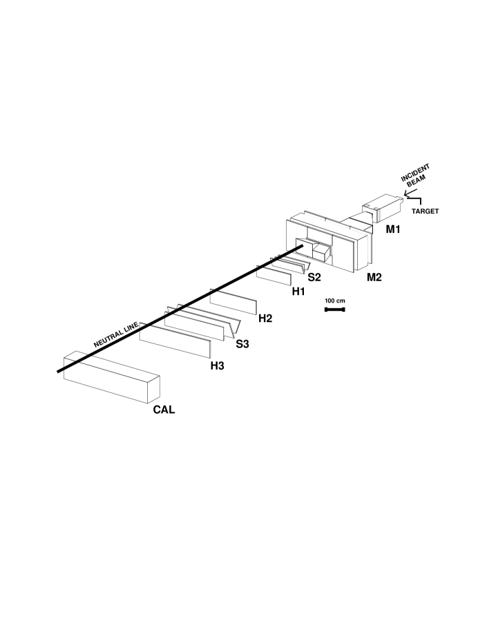
FIG. 1.: Perspective view of the E864 spectrometer. The vacuum tank is not shown.

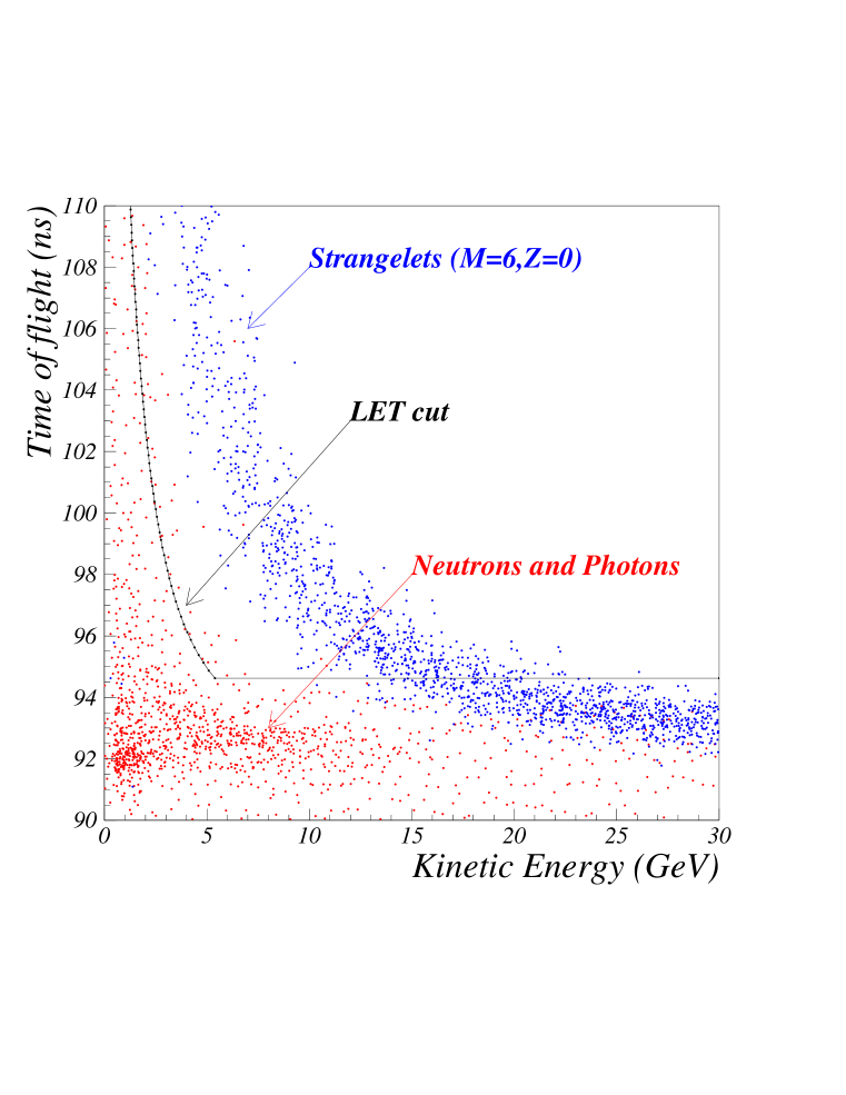
FIG. 2.: Simulation of the distribution of mass 6 uncharged strangelets, protons and neutrons in time versus energy space. The effects of detector resolution have been included. The solid curve illustrates a typical cut using the Late Energy Trigger (LET).

FIG. 3.: Acceptance of the spectrometer in transverse rigidity versus y for ${}^{6}He$ for a 1.5 T field. The acceptances are given in percent.

FIG. 4.: Particle identification using the charged particle tracking system. The average of the charges as determined by the three hodoscopes is plotted versus the mass/charge for positively charged tracks. Clear peaks for abundant particle species are apparent. A $\beta$ cut of $<0.985$ has been applied. The data are from a +1.5 T field run with the LET trigger set to enhance higher mass objects.

FIG. 5.: Single particle mass distributions for +1 charged particles at a 1.5 T field setting. A $\beta$ cut of 0.972 was applied. The data are from the 1996/7 run using the LET.

FIG. 6.: Single particle mass distribution for +2 charged particles at a 1.5 T field setting. The two curves demonstrate the effect of tightening the $\beta$ cut and adding calorimeter cuts.

FIG. 7.: Momentum resolution as a function of p for 0.2 T and 1.5 T magnetic fields.

FIG. 8.: Tracking mass vs. calorimeter mass distribution of charge=+1 candidates with $\beta\leq{0.972}$. Data points in the rectangles are for those candidates with mass greater than $5GeV/c^{2}$.

FIG. 9.: Mass distribution for Z=+3 strangelet candidates

FIG. 10.: 90% C.L. upper limits for the production of strangelets with positive charges per central $Au$ + $Pt$ collision at a beam momentum of 11.5 GeV/c per nucleon.

FIG. 11.: Charge -1 strangelet candidate distribution in calorimeter vs tracking mass. the cut at 5.0 GeV/$c^{2}$ for the minimum tracking mass is shown. The single candidate whose tracking and calorimeter mass agrees is circled

FIG. 12.: Charge -2 strangelet candidate distribution in tracking vs calorimeter mass

FIG. 13.: 90% C.L. upper limits for the production of strangelets with negative charges per central $Au$ + $Pt$ collision at a beam momentum of 11.5 GeV/c per nucleon.

FIG. 14.: Reconstructed mass spectrum of neutral particle candidates.

FIG. 15.: 90% C.L. upper limits for the production of neutral strangelets per central $Au$ + $Pt$ collision at a beam momentum of 11.5 GeV/c per nucleon.

FIG. 16.: Typical branching fraction limits for distillation of charged strangelets from a QGP

FIG. 17.: Branching fraction limits for distillation of neutral strangelets from a QGP.

FIG. 18.: Invariant yields at or near y = 1.9 and $p_{\perp}/A$ = 200 MeV/c as a function of mass number A.

REFERENCES

- [1] Formerly at Yale University and University of California at Los Angeles
- [2] Present address: University of Torino / INFN, Torino, Italy
- [3] Present address: Anderson Consulting, Hartford, CT
- [4] Present address: Univ. of Denver, Denver CO 80208
- [5] Deceased.
- [6] Present address: Cambridge Systematics, Cambridge, MA 02139
- [7] Formerly at Purdue University
- [8] Formerly at Yale University
- [9] Present address: McKinsey & Co., New York, NY 10022
- [10] Present address: Department of Radiation Oncology, Medical College of Virginia, Richmond VA 23298
- [11] Formerly at Yale University
- [12] Present address: University of Tennessee, Knoxville TN 37996
- [13] Present address: Lock Haven University, Lock Haven, PA 17745
- [14] Present address: Institut de Physique Nucleaire, 91406 Orsay Cedex, France
- [15] Present address: Institute for Defense Analysis, Alexandria VA 22311
- [16] Present address: MIT Lincoln Laboratory, Lexington MA 02173
- [17] Present address: Brookhaven National Laboratory, Upton, NY 11973
- [18] Present address: College of William and Mary, Williamsburg, VA 23185
- [19] Experiment E852: G.S. Adams et al., Phys. Rev. Lett. 81, 5760 (1998).
- [20] S. Chin and A. Kerman, Phys. Rev. Lett. 43, 1292 (1979).
- [21] A. Chodos, R.L. Jaffe, K. Johnson, C.B. Thorn and V.F. Weisskopf, Phys. Rev. D 9, 3471 (1974).
- [22] E. Farhi and R. Jaffe, Phys. Rev. D 30, 2379 (1984).
- [23] E. Gilson and R. Jaffe, Phys. Rev. Lett. 71, 332 (1993).
- [24] E. Witten, Phys. Rev. D 30, 272 (1984).
- [25] R.L. Jaffe, Phys. Rev. Lett. 38, 195 (1977).
- [26] J.F. Donoghue, E. Golowich and B.R. Holstein, Phys. Rev. D 34, 3434 (1986).
- [27] X.-D. Li, I. Bombaci, M. Dey, J. Dey and E.P.I. van den Heuvel, Phys. Rev. Lett. 83, 3776 (1999).
- [28] M.S. Berger and R. Jaffe, Phys. Rev. C 35, 213 (1987).
- [29] G.L. Shaw, M. Shin, R.H. Dalitz and M. Desai, Nature (London) 337, 436 (1989).
- [30] J. Schaffner, C.B. Dover, A. Gal, C. Greiner and H. Stocker, Phys. Rev. Lett. 71, 1328 (1993).
- [31] J. Madsen, Phys. Rev. Lett. 70, 391 (1993).
- [32] A.J. Baltz, C.B. Dover, S.H. Kahana, Y. Pang, T.J. Schlagel and E. Schnedermann, Phys. Lett. B 325, 7 (1994).
- [33] P. Braun-Munzinger, J. Stachel, J.P. Wessels, and N. Xu, Phys. Lett. B 365, 1 (1996).
- [34] J. Kapusta, A.P. Vischer and R. Venugopalan, Phys. Rev. C 51, 901 (1995); J. Kapusta and A. Vischer, Phys. Rev. C 52, 2725 (1995).
- [35] C. Greiner, P. Koch and H. Stocker, Phys. Rev. Lett. 58, 1825 (1987); C. Greiner and H. Stocker, Phys. Rev. D 44 3517 (1991).
- [36] H. C. Liu and G.L. Shaw, Phys. Rev. D 30, 1137 (1984).
- [37] H.J. Crawford, M.S. Desai and G.L. Shaw, Phys. Rev. D 45, 857 (1992).
- [38] J. Schaffner-Bielich, C. Greiner, A. Diener and H. Stocker, Phys. Rev. C 55, 3038 (1997).
- [39] T.K. Hemmick et al., Phys. Rev. D 41. 2074 (1990).
- [40] C. Alcock and A. Olinto, Ann. Rev. Nucl. Part. Sci. 38, 161 (1988).
- [41] Experiment E814: J. Barrette et al., Phys. Lett. B 252, 550 (1990).
- [42] Experiment E858: A. Aoki et al., Phys. Rev. Lett. 69, 2345 (1992).
- [43] Experiment NA52: K. Borer et al., Phys. Rev. Lett. 72, 1415 (1994).
- [44] Experiment E878: D. Beavis et al., Phys. Rev. Lett. 75, 3078 (1995); A. Rusek et al., Phys. Rev. C 54, R15 (1996).
- [45] Experiment NA52: G. Applequist et al., Phys. Rev. Lett. 76, 3907 (1996); G. Ambrosini et al., Nucl. Phys. A610, 306c (1996).
- [46] Experiment E836: R.W. Stotzer et al., Phys. Rev. Lett. 78, 3646 (1997).
- [47] Experiment E810: R. Longacre et al., Nucl. Phys. A590, 477c (1995).
- [48] Experiment E888: J. Belz et al., Phys. Rev. Lett. 76, 3277 (1996).
- [49] Experiment KTeV: A. Alavi-Harati et al., Phys. Rev. Lett. 84, 2593 (2000).
- [50] R. Klingenberg, J. Phys. G: Nucl. Part. Phys. 25, R273 (1999).
- [51] T.A. Armstrong et al., Phys. Rev. Lett. 79, 3612 (1997); T.A. Armstrong et al., Nucl. Phys. A625, 494 (1997).
- [52] T.A. Armstrong et al., Phys. Rev. C 59, R1829 (1999).
- [53] T.A. Armstrong et al., Nucl. Instrum. Methods Phys. Res. A 437, 222 (1999).
- [54] P. Haridas et al., Nucl. Instrum. Methods Phys. Res. A 385, 412 (1997).
- [55] T.A. Armstrong et al., Nucl. Instrum. Methods Phys. Res. A 425, 210 (1999).
- [56] D. Acosta et al., Nucl. Instrum. Methods Phys. Res. A 308, 481 (1991); D. Acosta et al., Nucl. Instrum. Methods Phys. Res. A 316, 184 (1992).
- [57] T.A. Armstrong et al., Nucl. Instrum. Methods Phys. Res. A 406, 227 (1998).
- [58] J.G. Lajoie, Ph.D. Thesis, Yale University (1996).
- [59] J.G. Lajoie, Proceedings of the 1995 IEEE Conference on Real-Time Applications in Nuclear, Particle and Plasma Physics.
- [60] J.C. Hill et al., Nucl. Instrum. Methods Phys. Res. A 421, 431 (1999).
- [61] R. Brun et al., GEANT 3.12 User’s Guide, CERN Data Handling Division, DD/EE/84-1.
- [62] A. Chikanian, B.S. Kumar, N. Smirnov and E. O’Brien, Nucl. Instrum. Methods Phys. Res. A 371, 480 (1996).
- [63] M.G. Munhoz, Ph.D. thesis, University of Sao Paulo (1999); H. Jaradat, Ph.D. thesis, Wayne State University (2000).
- [64] G. Ambrosini et al., Nucl. Phys. A610, 306c (1996).
- [65] Z. Xu, Ph.D. thesis, Yale University (1999).
- [66] G.E. Van Buren, Ph.D. thesis, Massachusetts Institute of Technology (1998).
- [67] W.A. Gale and I.M. Duck, Nucl. Phys. B8, 109 (1968).
- [68] G.Kalbermann and J.M. Eisenberg, J. Phys. G 5, 35 (1978).
- [69] T.E.O. Ericson and F. Myhrer, Phys. Lett. B 74, 163 (1978).
- [70] E. Freidman, A. Gal, and V.B. Mandelzweig, Phys. Rev. Lett. 41, 794 (1978).
- [71] H. Garcilazo, Phys. Rev. C 26, 2685 (1982); Phys. Rev. Lett. 50, 1567 (1983).
- [72] F.W.N. de Boer et al,, Phys. Rev. Lett. 53, 423 (1984).
- [73] D. Ashery et al., Phys. Lett. B 215, 41 (1988).
- [74] N. Willis et al., Phys. Lett. B 229, 33 (1989).
- [75] B. Parker, K.K. Seth, C.M. Ginsberg, B. O’Reilly, M. Sarmiento, R. Soundranayagam and S. Trokenheim, Phys. Rev. Lett. 63, 1570 (1989).
- [76] F.W.N. de Boer, Phys. Rev. D 43, 3063 (1991).
- [77] J. Barrette et al., Phys. Rev. C 52, 2679 (1995).
- [78] T. Suzuki, M. Fujimaki, S. Hirenzaki, N. Inabe, T. Kobayahi, T. Kubo, T. Nakagawa, Y. Watanabe, I. Tanihata and S. Shimoura, Phys. Rev. C 47, 2673 (1993).
- [79] D.E. Kahana, S.H. Kahana, Y. Pang, A.J. Baltz, C.B. Dover, E. Schnedermann and T.J. Schagel, Phys. Rev. C 54, 338 (1996).
- [80] T.A. Armstrong et al., Phys. Rev. C, 61, 064908 (2000).
- [81] T.A. Armstrong et al., Phys. Rev. C, to be published.