Pion Imaging at the AGS

Abstract

Source imaging analysis was performed on two-pion correlations in central Au + Au collisions at beam energies between 2 and 8$A$ GeV. We apply the imaging technique by Brown and Danielewicz, which allows a model-independent extraction of source functions with useful accuracy out to relative pion separations of about 20 fm. We found that extracted source functions have Gaussian shapes. Values of source functions at zero separation are almost constant across the energy range under study. Imaging results are found to be consistent with conventional source parameters obtained from a multidimensional HBT analysis.

I Introduction

Measurements of two-particle correlations offer a powerful tool for studies of spatial and temporal behaviour of the heavy-ion collisions. The complex nature of the heavy-ion reactions requires utilization of different probes and different analysis techniques in order to obtaine reliable and complete picture of the system created in the collision.
We will discuss application of imaging technique of Brown-Danielewicz which allows one to reconstruct the entire source function, phase space density and entropy from any like-pair correlations in a model independent way. We will present recent results of the two-pion imaging analysis performed by the E895 Collaboration and discuss natural connection between imaging and traditional HBT.

A E895 Experiment and Analysis Details

Detailed description of the experiment E895 can be found elsewhere [1]. The Au beams of kinetic energy 1.85, 3.9, 5.9 and 7.9$A$ GeV from the AGS accelerator at Brookhaven were incident on a fixed Au target. The analyzed $\pi^{-}$ samples come from the main E895 subsystem — the EOS Time Projection Chamber (TPC) [2], located in a dipole magnetic field of 0.75 or 1.0 Tesla. Results of the E895 $\pi^{-}$ HBT analysis were reported earlier [3], and in this paper, we focus on an application of imaging to the same datasets.

B Source Imaging

In order to obtain the two-pion correlation function $C_{2}$ experimentally, the standard event-mixing technique was used [4]. Negative pions were detected and reconstructed over a substantial fraction of $4\pi$ solid angle in the center-of-mass frame, and simultaneous measurement of particle momentum and specific ionization in the TPC gas helped to separate $\pi^{-}$ from other negatively charge particles, such as electrons, K^- and antiprotons. Contamination from these species is estimated to be under 5%, and is even less at the lower beam energies and higher transverse momenta. Momentum resolution in the region of correlation measurements is better than 3%. Event centrality selection was based on the multiplicity of reconstructed charged particles. In the present analysis, events were selected with a multiplicity corresponding to the upper 11% of the inelastic cross section for Au + Au collisions. Only pions with $p_{T}$ between 100 MeV/$c$ and 300 MeV/$c$ and within $\pm 0.35$ units from midrapidity were used. Another requirement was for each used $\pi^{-}$ track to point back to the primary event vertex with a distance of closest approach (DCA) less than 2.5 cm. This cut removes most pions originating from weak decays of long-lived particles, e.g. $\Lambda$ and K⁰. Monte Carlo simulations based on the RQMD model [5] indicate that decay daughters are present at a level that varies from 5% at 4$A$ GeV to 10% at 8$A$ GeV, and they lie preferentially at $p_{T}<100$ MeV/$c$. Finally, in order to overcome effects of track merging, a cut on spatial separation of two tracks was imposed. For pairs from both “true” and “background” distributions, the separation between two tracks was required to be greater than 4.5 cm over a distance of 18 cm in the beam direction. This cut also suppresses effects of track splitting [3]. Correlation functions were corrected for pion Coulomb interaction [3].

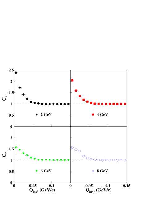
FIG. 1.: Measured two-pion correlation functions for Au + Au central collisions at four beam energies.

Imaging [6, 7] was used to extract quantitative information from the measured correlation functions. It has been shown [8] that imaging allows robust reconstruction of the source function for systems with non-zero lifetime, even in the presence of strong space-momentum correlations. The main features of the method are outlined below; see Refs [6, 7, 9] for more details. The two-particle correlation function may be expressed as follows:

$$C_{\bf P}({\bf Q})-1=\int d{\bf r}\,K({\bf Q},{\bf r})\,S_{\bf P}({\bf r})\,,$$ (1)

where $K=|\Phi_{\bf Q}^{(-)}({\bf r})|^{2}-1$ and $\Phi_{\bf Q}^{(-)}$ is the relative wavefunction of the pair. The source function, $S_{\bf P}({\bf r})$, is the distribution of relative separations of emission points for the two particles in their center-of-mass frame. The total momentum of the pair is denoted by ${\bf P}$, the relative momentum by ${\bf Q}={\bf p_{1}}-{\bf p_{2}}$, and the relative separation by ${\bf r}$. Since the correlation data is already Coulomb corrected, we may approximate the relative wavefunction of the pions with a noninteracting spin-0 boson wavefunction:

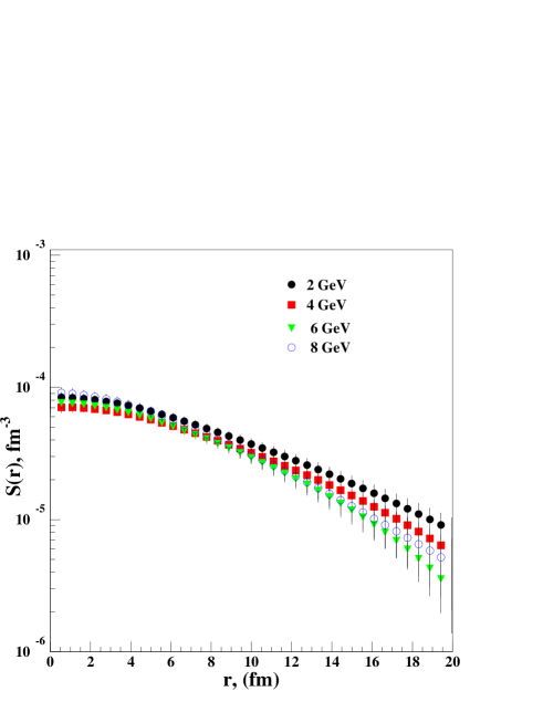
FIG. 2.: Relative source functions extracted from the pion correlation data at 2, 4, 6 and 8$A$ GeV.

$$\Phi_{{\bf Q}}^{(-)}({\bf r})=\frac{1}{\sqrt{2}}\left(e^{i{\bf Q}/2\cdot{\bf r}}+e^{-i{\bf Q}/2\cdot{\bf r}}\right).$$ (2)

The goal of imaging is the determination of the relative source function ($S_{\bf P}({\bf r})$ in Eq. (1)), given $C_{\bf P}({\bf Q})$. The problem of imaging then becomes the problem of inverting $K({\bf q},{\bf r})$ [10]. For pions, one might think that because Eq. 1 is a Fourier cosine transform it may be inverted analytically [6] to give the source function directly in terms of the correlation function:

TABLE I.: Radius parameters of Gaussian fits to the extracted source ($R_{S}$) functions and measured correlation functions($R_{C2}$) for different energies.

$E_{b}$ (AGeV)	2	4	6	8
$R_{S}$(fm)	6.70$\pm$0.04	6.35$\pm$0.03	5.56$\pm$0.03	5.53$\pm$0.05
$R_{C2}$ (fm)	6.39$\pm$0.2	6.05$\pm$0.1	5.51$\pm$0.15	5.61$\pm$0.28

$$S_{\bf p}({\bf r})=\frac{1}{(2\pi)^{3}}\int d^{3}{Q}\,\cos{({\bf Q}\cdot{\bf r})}\left(C_{\bf p}({\bf Q})-1\right).$$ (3)

While this might work for vanishing experimental uncertainty, for realistic situations, this is a poor way to perform the inversion. When Fourier transforming, it is impossible to distinguish between statistical noise and real structure in the data [11]. Instead, we proceed as in [13] and expand the source in a Basis Spline basis: $S({\bf r})=\sum_{j}S_{j}B_{j}({\bf r})$. With this, Eq. (1) becomes a matrix equation $C_{i}=\sum_{j}K_{ij}S_{j}$ with a new kernel:

$$K_{ij}=\int d{\bf r}K({\bf Q}_{i},{\bf r})B_{j}({\bf r}).$$ (4)

Imaging reduces to finding the set of source coefficients, $S_{j}$, that minimize the $\chi^{2}$. Here, $\chi^{2}=\sum_{i}(C_{i}-\sum_{j}K_{ij}S_{j})^{2}/\Delta^{2}C_{i}$.
This set of source coefficients is $S_{j}=\sum_{i}[(K^{T}(\Delta^{2}C)^{-1}K)^{-1}K^{T}B]_{ji}(C_{i}-1)$ where $K^{T}$ is the transpose of the kernel matrix. The uncertainty of the source is the square-root of the diagonal elements of the covariance matrix of the source, $\Delta^{2}S=(K^{T}(\Delta^{2}C)^{-1}K)^{-1}$. It has been shown [9] that for the case of noninteracting spin-zero bosons with Gaussian correlations, there is a natural connection between the imaged sources and “standard” HBT parameters. Indeed, the source is a Gaussian with the “standard” HBT parameters as radii:

$$S({\bf r})=\frac{\lambda}{(2\sqrt{\pi})^{3}\sqrt{\det{[R^{2}]}}}\exp{\left(-\frac{1}{4}r_{i}r_{j}[R^{2}]^{-1}_{ij}\right)}\,,$$ (5)

where $\lambda$ is a fit parameter traditionally called the chaoticity or coherence factor in HBT analyses. Here, $[R^{2}]$ is the real symmetric matrix of radius parameters

$$[R^{2}]=\left(\begin{array}[]{ccc}R_{o}^{2}&R_{os}^{2}&R_{o\ell}^{2}\\ R_{os}^{2}&R_{s}^{2}&R_{s\ell}^{2}\\ R_{o\ell}^{2}&R_{s\ell}^{2}&R_{\ell}^{2}\end{array}\right).$$ (6)

Eq. (5) is the most general Gaussian one may use, but usually one assumes a particular symmetry of the single particle source so that there is only one non-vanishing non-diagonal element $R_{ol}^{2}$. The asymptotic value of the relative source function at zero separation $S({\bf r}\rightarrow 0)$ is related to the inverse effective volume of particle emission, and has units of fm^-3:

$$S({\bf r}\rightarrow 0)=\frac{\lambda}{(2\sqrt{\pi})^{3}\sqrt{\det{[R^{2}]}}}\,.$$ (7)

As it was shown in [9] $S({\bf r}\rightarrow 0)$ is an important parameter needed to extract the space-averaged phase-space density. Figure 1 shows measured angle-averaged two-pion correlation functions for central Au + Au collisions at 2, 4, 6 and 8$A$ GeV. Figure 2 shows relative source functions $S(r)$ obtained by applying the imaging technique to the measured two-pion correlation functions. Note that the plotted points are for representation of the continuous source function and hence are not statistically independent of each other as the source functions are expanded in Basis Splines [13]. Since the source covariance matrix is not diagonal, the coefficients of the Basis spline expansion are also not independent which is taken into account during $\chi^{2}$ calculations.

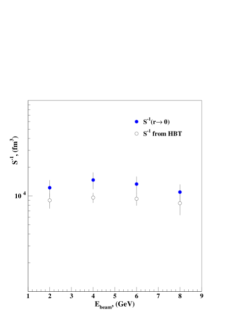
FIG. 3.: Values of inverse relative source functions at zero separation as a function of beam energy, obtained using imaging (solid circles) and HBT (open circles).

TABLE II.: Fit parameters for the Bertsch-Pratt HBT parameterization of the pion correlation functions for E895 beam energies used for evaluation of $S(r\rightarrow 0)$.

$E_{b}$ (AGeV)	2	4	6	8
$\lambda$	0.99$\pm$0.06	0.74$\pm$0.03	0.65$\pm$0.03	0.65$\pm$0.05
$R_{o}$ (fm)	6.22$\pm$0.26	5.79$\pm$0.16	5.76$\pm$0.23	5.49$\pm$0.31
$R_{s}$ (fm)	6.28$\pm$0.20	5.37$\pm$0.11	5.05$\pm$0.12	4.83$\pm$0.21
$R_{l}$ (fm)	5.15$\pm$0.19	5.15$\pm$0.14	4.72$\pm$0.18	4.64$\pm$0.24
$R_{ol}^{2}$ (fm)	-2.43$\pm$1.71	0.43$\pm$1.03	2.17$\pm$1.20	-0.65$\pm$1.85

With this technique, we may reconstruct the distribution of relative pion separations with useful accuracy out to $r\sim 20$ fm. The images obtained at each of the four E895 beam energies are rather similar in shape, and upon fitting with a Gaussian function, values of $\chi^{2}$ per degree of freedom between 0.9 and 1.2 are obtained. Results of fits to the source function and correlation functions are shown in Table I. One can see that source radii extracted via both techniques are similar, further confirming the validity of a Gaussian source hypothesis. Figure 3 compares values related to effective volumes of pion emission inferred from the standard Bertsch-Pratt pion HBT parametrization (open circles) with the effective volumes derived from the image source functions shown in Fig. 2 (solid circles). Essentially, this figure plots the inverse of the left- and right-hand sides of Eq. 7. Results of the multidimensional Bertsch-Pratt fit to the pion correlation data have already been published in Ref. [3] and are reproduced in Table II. It can be seen from Fig. 3 that the agreement between imaging and the HBT parametrization is fairly good. Values of source functions at zero separations estimated via either technique are approximately constant within errors across the 2 to 8$A$ GeV beam energy range.
In summary, we present measurements of one-dimensional correlation functions for negative pions emitted at mid-rapidity from central Au + Au collisions at 2, 4, 6 and 8$A$ GeV. These correlation functions are analyzed using the imaging technique of Brown and Danielewicz. It is found that relative source functions $S(r)$ have rather similar shapes and zero-separation intercepts $S(r\rightarrow 0)$. Distributions of relative separation have been measured out to 20 fm, and the extracted source functions are approximately Gaussian. We have performed the first experimental check of the predicted connection between imaging and traditional meson interferometry techniques and found that the two methods are in good agreement. This agreement paves the way for applications of the imaging method to the interpretation of pair correlations among strongly interacting particle such as protons, antiprotons, etc. Values of source functions at zero separation which are related to the pion effective volumes of emission are almost constant across the range of bombarding energies under study.

REFERENCES

- [1] G. Rai et al., proposal LBL-PUB-5399 (1993).
- [2] G. Rai et al., IEEE Trans. Nucl. Sci. 37, 56 (1990).
- [3] E895 Collaboration, M.A. Lisa et al., Phys. Rev. Lett. 84, 2798 (2000).
- [4] G. Kopylov, Phys. Lett. 50B, 472 (1974).
- [5] H. Sorge, Phys. Rev. C 52, 3291 (1995).
- [6] D.A. Brown and P. Danielewicz, Phys. Lett. B398, 252 (1997).
- [7] D.A. Brown and P. Danielewicz, Phys. Rev. C57, 2474 (1998).
- [8] S.Y. Panitkin and D.A. Brown, Phys. Rev. C61, 021901 (2000).
- [9] D.A. Brown, S.Y. Panitkin and G.F. Bertsch, Phys. Rev. C62, 014904 (2000).
- [10] A. Tarantola, Inverse Problem Theory, Elsevier, (1987).
- [11] D. Brown, nucl-th/9904063.
- [12] D.A. Brown, nucl-th/0003021.
- [13] D.A. Brown and P. Danielewicz, in preparation; C. de Boor, A Practical Guide to Splines, Springer-Verlag, (1978).