Monitoring of the accelerator beam distributions for internal target facilities

Abstract

We describe a direct method for monitoring the geometrical dimensions of a synchrotron beam at the target position for internal target installations. The method allows for the observation of the proton beam size as well as the position of the beam relative to the target. As a first demonstration of the technique, we present results obtained by means of the COSY-11 detection system installed at the cooler synchrotron COSY. The influence of the stochastic cooling on the COSY proton beam dimensions is also investigated.

, , , , , , , , , , , , , , , , , , , , ,

1 Introduction

Internal cluster target facilities – such as COSY-11 [1] installed at the cooler synchrotron COSY-Jülich [2] – permit the study of the production of mesons in the proton-proton interaction with high luminosity ($10^{~{}31}$ cm^-2 s^-1) in spite of very low target densities ($\approx 10^{~{}14}$ atoms cm^-2). Such conditions minimize changes in the ejectiles’ momentum vectors due to secondary scattering in the target, and hence facilitate the precise study of reactions with cross section values at the nanobarn level.

An exact extraction of absolute cross sections from the measured data demands a reliable estimation of the acceptance of the detection system. This in turn crucially depends on the accuracy of the determination of the position and dimensions of both the beam and the target. Using the COSY–11 detection system [1] as illustration, we will describe a method for estimating the dimensions of the proton beam, based on the momentum distribution for elastically scattered protons, which can be measured simultaneously with the investigated reaction.

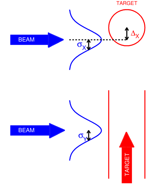
Figure 2: Schematic depiction of the relative beam and target setting. Seen from above (upper part), and from aside (lower part), $\sigma_{X}$ and $\sigma_{Y}$ denote the horizontal and vertical standard deviation of the assumed Gaussian distribution of the proton beam density, respectively. The distance between the centres of the proton and the target beam is described as $\Delta_{X}$.

At the COSY–11 facility (see Fig. 1) the production of short-lived uncharged mesons ($\eta$, $\omega$, $\eta^{\prime}$, or $\phi$) and hyperons ($\Lambda$ and $\Sigma^{0}$) is investigated by means of the missing mass technique via the $pp\rightarrow ppX$ and $pp\rightarrow pK^{+}Y$ reactions, respectively [3, 4, 5]. In this way, the four-momenta of positively charged particles are fully determined experimentally. The accuracy of the extracted missing mass value determines whether the signal from the given meson is visible over a background and depends on the precision of the momentum reconstruction of the registered protons or kaons. Consequently, it varies with the detector resolution, the momentum spread and the geometrical spread of the accelerator proton beam interacting with the internal cluster target beam. The momentum reconstruction is performed by tracing back trajectories from drift chambers through the dipole magnetic field to the target (Fig. 1,[1]), which is an infinitely thin vertical line in the ideal case. In reality, however, the reactions take place in a region of finite dimensions where the beam and the target overlap (see Fig. 2). Assuming an infinitesimal target, our analysis shows a smearing out of the momentum vectors and hence of the resolution of the missing mass signal. However, if the target and beam dimensions are known it is possible to determine the average smearing of the missing mass originating from this effect and hence to infer for example the natural width of the measured mesons, provided that the beam momentum spread is known as well.

2 Description of the method

Part of the COSY–11 detection setup used for the registration of elastically scattered protons is shown in Figure 1. Trajectories of protons scattered in the forward direction are measured by means of two drift chambers (D1 and D2) and a scintillator hodoscope (S1), whereas the recoil protons are registered in coincidence with the forward ones using a silicon pad detector arrangement (Si) and a scintillation detector (S4). The two–body kinematics gives an unambiguous relation between the scattering angles $\Theta_{1}$ and $\Theta_{2}$ of the recoil and forward protons (see Fig. 1). Therefore, as seen in Figure 3, events of elastically scattered protons can be identified from the correlation line formed between the position in the silicon pad detector Si, and the scintillator hodoscope S1, the latter measured by the two drift chamber stacks. For those protons which are elastically scattered in the forward direction and deflected in the magnetic field of the dipole, the momentum vector at the target point can be determined. According to two–body kinematics, momentum components parallel and perpendicular to the beam axis form an ellipse. A section of this ellipse is shown as a solid line in Figure 4a superimposed on the data which were selected according to the correlation criterion from Figure 3 for elastically scattered events.

In Figures 3 and Figure 4a, the elastically scattered events stand out clearly against a low level background. But more importantly the mean of the elastically scattered data is significantly shifted from the expected line, indicating that the reconstructed momenta are on average larger than expected. This discrepancy is difficult to explain in terms of the uncertainties of either the proton beam momentum or the proton beam angle. For instance, to account for this discrepancy, the beam momentum must be changed by more than 120 MeV/c (dashed line in Figure 4a), which is 40 times larger than the conservatively estimated error of the absolute beam momentum ($\pm$ 3 MeV/c) [6, 7]. Similarly, the effect could have been corrected by changing the beam angle by 40 mrad (see dotted line in Figure 4a), which exceeds the uncertainty of the beam angle ($\pm$ 1 mrad [6]) by at least a factor of 40.

A reasonable agreement is obtained, however, by shifting the assumed reaction point relative to the nominal value by $-0.2$ cm perpendicular to the beam axis towards the center of the COSY–ring, along the X-axis defined in Figure 1. The experimentally extracted momentum components obtained in this manner are shown in Figure 4b, together with the expectation depicted by the solid line. There is good agreement and the data are now spread symmetrically around the ellipse. This spread is essentially due to the finite extensions of the cluster target and the proton beam overlap (about $\pm 0.2$ cm as inferred from the shift in the target position required). Other contributions, including the spread of the beam momentum and still some multiple scattering events, appear to be negligible. We now consider in more detail the influence of the effective target dimensions and the spread of the COSY beam.

We assume the target beam to be described by a cylindrical pipe, with a diameter of 9 mm, homogeneously filled with protons [8, 9]. Furthermore, the COSY proton beam density distribution is described by Gaussian functions with standard deviations $\sigma_{X}$ and $\sigma_{Y}$ for the horizontal and vertical directions (see Fig. 2), respectively [10, 11]. Monte–Carlo calculations are performed varying the distance between the target and the beam centres ($\Delta_{X}$), and the horizontal proton beam extension ($\sigma_{X}$).

In order to account for the angular distribution of the elastically scattered protons, an appropriate weight $w$ was assigned to each generated event according to the differential distributions of the cross sections measured by the EDDA collaboration [12]. The generated events were analyzed in the same way as the experimental data. A comparison of the data from Figure 4a (data analyzed using the nominal interaction point) with the corresponding simulated histograms allows both $\sigma_{X}$ and $\Delta_{X}$ to be determined. For finding an estimate of the parameters $\sigma_{X}$ and $\Delta_{X}$ we construct the $\chi^{2}$ statistic according to the method of least squares:

$$\chi^{2}=\sum_{i}\,\frac{\left(\alpha N_{i}^{s}+b_{i}-N_{i}^{e}\right)^{2}}{\alpha^{2}\displaystyle\sum_{i^{th}bin}w^{2}+N_{i}^{e}+b_{i}},$$ (1)

where $N_{i}^{e}$ and ${\displaystyle N_{i}^{s}=\sum_{i^{th}bin}w}$ denote the content of the $i^{th}$ bin of the P_⟂–versus–P_∥ spectrum determined from experiment (Fig. 4a) and simulations, respectively. The background events $b_{i}$ in the i^th bin amount to less than one per cent of the data [13] and were estimated by linear interpolations between the inner and outer part of a broad distribution surrounding the expected ellipse originating from elastically scattered protons. The free parameter $\alpha$ allows adjustment of the overall scale of the fitted Monte–Carlo histograms. Thus, by varying the $\alpha$ parameter, the $\chi^{2}_{min}$ for each pair of $\sigma_{X}$ and $\Delta_{X}$ was established as a minimum of the $\chi^{2}(\alpha)$ distribution.

The results of the Monte–Carlo calculations are shown in Figure 5.
Figure 5a shows the logarithm of $\chi^{2}_{min}$ as a function of the values of $\sigma_{X}$ and $\Delta_{X}$. The $\chi^{2}_{min}$ function has a valley identifying a minimum and allowing the unique determination of the varied parameters $\sigma_{X}$ and $\Delta_{X}$. The overall minimum of the $\chi^{2}_{min}(\sigma_{X},\Delta_{X})$–distribution, at $\sigma_{X}$ = 0.2 cm and $\Delta_{X}$ = - 0.2 cm is more evident in Figures 5b and 5c, which show the projections of the valley line onto the respective axis.

The same results were obtained when employing the Poisson likelihood $\chi^{2}$ derived from the maximum likelihood method [14, 15]

$$\chi^{2}=2\cdot\sum_{i}\,[\alpha N_{i}^{s}+b_{i}-N_{i}^{e}+N_{i}^{e}\,ln(\frac{N_{i}^{e}}{\alpha N_{i}^{s}+b_{i}})],$$ (2)

The vertical beam extension of $\sigma_{Y}$ = 0.51 cm was established directly from the distribution of the vertical component of the particle trajectories at the centre of the target. This is possible, since for the momentum reconstruction only the origin of the track in the horizontal plane is used, while the vertical component remains a free parameter. As shown in Figure 6, the reconstructed distribution of the vertical component of the reaction points indeed can be described well by a Gaussian distribution with the $\sigma$ = 0.53 cm. The width of this distribution is primarily due to the vertical spread of a proton beam. The spread caused by multiple scattering and drift chambers resolution was determined to be about 0.13 cm (standard deviation) [13]. Therefore, $\sigma_{Y}~{}=~{}\displaystyle\sqrt{\displaystyle 0.53^{2}-0.13^{2}}~{}\approx$ 0.51 cm.

The effect of a possible drift chamber misalignment, i. e. an inexactness of the angle $\beta$ in Figure 1, was estimated to cause a shift in the momentum plane by 0.15 cm for $\Delta_{X}$. This gives a rather large systematical bias in the estimation of the absolute value of $\Delta_{X}$, but it does not affect the parameter $\sigma_{X}$, and still allows for the determination of relative beam shifts $\Delta_{X}$ during the measurement cycle.

3 Monitoring of the beam geometry during the measurement cycle

It is possible to use the method described here to control the size and position of the beam relative to the target. This was demonstrated during the experimental run performed in February 1998 [5], when for the first time longitudinal and horizontal stochastic cooling were used at the COSY accelerator.
The horizontal stochastic cooling [10] is used to squeeze the proton beam in the horizontal direction until the beam reaches the equilibrium between the cooling and the heating due to the target. The size of an uncooled beam increases during the cycle, as can be seen in Figure 7a, which shows the spreading of the beam in the vertical plane during the 60 minutes cycle. This was expected since stochastic cooling in the vertical plane was not used in this case. The influence of the applied cooling in the horizontal plane is clearly visible in Figure 7b. During the first five minutes of the cycle the horizontal size of the beam of about $2\cdot 10^{10}$ protons was reduced by a factor of 2, reaching the equilibrium conditions, and remaining constant for the rest of the COSY cycle.

Figure 8 depicts the accuracy of the momentum reconstruction, reflected in the spread of the data, which is mainly due to the finite horizontal size of the beam and target overlap. The upper and lower panel correspond to the first and the last minute of the measurement cycle, respectively. The data were analyzed correcting for the relative target and beam shifts $\Delta_{X}$ as determined by the method discussed above. The movement of the beam relative to the target during the cycle is quantified in Figure 7c. The shift of the beam denotes also changes of the average beam momentum, due to the nonzero dispersion at the target position. The beam reaches stability after some minutes. This can be understood as the equilibration between the energy losses when crossing $1.6\cdot 10^{6}$ times per second through the $H_{2}$ cluster target, and the power of the longitudinal stochastic cooling which can not only diminish the spread of the beam momentum but also shifts it as a whole.

4 Conclusions

We presented a method which allows the proton beam dimensions and its position relative to the target to be controlled for internal beam experimental facilities. The technique is based on the measurements of the momentum distribution of elastically scattered protons and its comparison with the distributions simulated with different beam and target conditions. We demonstrated the applicability of the method in controlling the proton beam during measurement when stochastic cooling was used at the synchrotron COSY for the first time.

Acknowledgements
One of the authors (P.M.) acknowledges hospitality and financial support from the Forschungszentrum Jülich. We appreciate the careful reading of the manuscript by J.N. Tan.
This research project was supported in part by the BMBF (06MS881I), the Bilateral Cooperation between Germany and Poland represented by the Internationales Büro DLR for the BMBF (PL-N-108-95) and by the Polish State Committee for Scientific Research, and by FFE grants (41266606 and 41266654) from the Forschungszentrum Jülich.

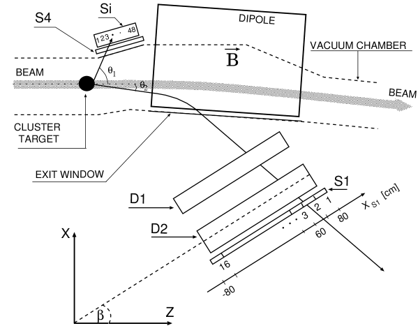
Figure 1: Schematic diagram of the COSY–11 detection setup. Only detectors used for the measurement of elastically scattered protons are shown. Numbers used on the silicon pad detector (Si) and below the scintillator hodoscope (S1) indicate the order of segments. D1 and D2 denote drift chambers. The X_S1 axis is defined such that the first segment of the S1 ends at 80 cm and the sixteenth ends at -80 cm. The proton beam, depicted by a shaded line, circulates in the ring and crosses each time the $H_{2}$ cluster target installed in front of one of the bending dipole magnets of the COSY accelerator.

Figure 3: Identification of elastically scattered protons from the correlation of hits in the silicon detector Si and the S1 scintillator hodoscope. Note that the number of entries per bin is given in a logarithmic scale, ranging from 1 (smallest box) to 19000 (largest box).

Figure 4: a)   Perpendicular versus parallel momentum components with respect to the beam direction of particles registered at a beam momentum of 3.227 GeV/c. The number of entries per bin is shown logarithmically. The solid line corresponds to the momentum ellipse expected for elastically scattered protons at a beam momentum of 3.227 GeV/c, the dashed line refers to a beam momentum of 3.350 GeV/c, and the dotted line shows the momentum ellipse obtained for a proton beam inclined by 40 mrad.
b )    The same data as shown in a) but analyzed with the target point shifted by -0.2 cm perpendicularly to the beam direction (along the X-axis in Figure 1). The solid line shows the momentum ellipse at a beam momentum of 3.227 GeV/c.

Figure 5: a) $\chi^{2}_{min}$ as a function of $\sigma_{X}$ and $\Delta_{X}$. The number of entries is shown in a logarithmic scale.   b) $\chi^{2}_{min}$ as a function of $\Delta_{X}$.    c) $\chi^{2}_{min}$ as a function of $\sigma_{X}$.  The minimum value of $\chi^{2}_{min}$ is larger than two. However, it decreases when only a part of the 60 minutes long COSY cycle is taken into account (see section 3). This is due to the fact that the beam changes during the cycle and its form, when integrated over the whole cycle time, does not suit perfectly to the form assumed in Monte–Carlo simulations.

Figure 6: Distribution of the vertical component of the reaction points determined by tracing back trajectories from the drift chambers through the dipole magnetic field to the centre of the target (in the horizontal plane). “Tails” are due to secondary scattering on the vacuum chamber and were parametrized by a polynomial of second order. The solid line shows the simultaneous fit of the Gaussian distribution and the polynomial of second order.

Figure 7: The vertical a) and horizontal b) beam width (one standard deviation) determined for each five minutes partition of the COSY cycle.
Note that the beam width $\sigma_{X}$ determined for each five minutes period is smaller than the $\sigma_{X}$ averaged over the whole cycle (compare Figure 5c). This is due to the beam shift relative to the target during the experimental cycle as shown in the panel on the bottom left.
c) Relative settings of the COSY proton beam and the target centre versus the time of the measurement cycle. d) Changes of the luminosity during the cycle. A steep decrease on the beginning is caused by the movement of the beam out from the target centre.
The vertical error bars in pictures b) and c) denote the size of the step used in the Monte-Carlo simulations ($\pm$ 0.025 cm ; the bin width of Figures 5b and 5c).

Figure 8: Perpendicular versus parallel momentum components with respect to the beam direction of particles registered at a beam momentum of 3.227 GeV/c, as measured during the first minute (a), and the last minute (b) of the 60 minutes long COSY cycle. The data at the first minute were analyzed with $\Delta_{X}$ = -0.15 cm, and the data of the 60’s minute with $\Delta_{X}$ = -0.25 cm, see figure 7c. The number of entries per bin is shown on a logarithmic scale. The solid line corresponds to the momentum ellipse expected for protons scattered elastically at a beam momentum of 3.227 GeV/c.

References

- [1] S. Brauksiepe et al., Nucl. Instr. & Meth. A 376 (1996) 397.
- [2] R. Maier, Nucl. Instr. Meth. A 390 (1997) 1.
- [3] S. Sewerin et al., Phys. Rev. Lett. 83 (1999) 682.
- [4] J. Smyrski et al., Phys. Lett. B 474 (2000) 182.
- [5] P. Moskal et al., Phys. Lett. B 474 (2000) 416.
- [6] D. Prasuhn, R. Stassen, private communications.
-
[7]
P. Moskal et al., Annual Report 1997, IKP, FZ Jülich,
Jül-3505 (1998) 41.
http://ikpe1101.ikp.kfa-juelich.de/
/cosy-11/pub/ListofPublications.htmlreps - [8] H. Dombrowski et al., Nucl. Instr. & Meth. A 386 (1997) 228.
- [9] A. Khoukaz et al., Eur. Phys. J. D 5 (1999) 275.
- [10] D. Prasuhn et al., Nucl. Instr. & Meth. A 441 (2000) 167.
-
[11]
M. Schulz-Rojahn, doctoral thesis,
Rheinische Friedrich-Wilhelm-Universität Bonn (1998). - [12] D. Albers et al., Phys. Rev. Lett. 78 (1997) 1652.
-
[13]
P. Moskal, doctoral thesis, Jagellonian University, Cracow 1998,
IKP FZ Jülich, Jül-3685, August 1999, http://ikpe1101.ikp.kfa-juelich.de/ - [14] S. Baker, R.D. Cousins, Nucl. Instr. & Meth. 221 (1984) 437.
- [15] G.J. Feldman, R.D. Cousins, Phys. Rev. D 57 (1998) 3873.