Measurement of the charged pion electromagnetic form factor

Abstract

Separated longitudinal and transverse structure functions for the reaction ¹H$(e,e^{\prime}\pi^{+})n$ were measured in the momentum transfer region $Q^{2}$ = 0.6 - 1.6 $\text{(GeV}/c\text{)}^{2}$ at a value of the invariant mass $W=1.95$ GeV. New values for the pion charge form factor were extracted from the longitudinal cross section by using a recently developed Regge model. The results indicate that the pion form factor in this region is larger than previously assumed and is consistent with a monopole parameterization fitted to very low $Q^{2}$ elastic data.

The pion occupies an important place in the study of the quark-gluon structure of hadrons. This is exemplified by the many calculations that treat the pion as one of their prime examples [1] –[8]. One of the reasons is that the valence structure of the pion, being $\langle q\bar{q}\rangle$, is relatively simple. Hence it is expected that the value of the four-momentum transfer squared $Q^{2}$, down to which a pQCD approach to the pion structure can be applied, is lower than e.g. for the nucleon. Furthermore, the asymptotic normalization of the pion wave function, in contrast to that of the nucleon, is known from the pion decay.

The charge form factor of the pion, $F_{\pi}(Q^{2})$, is an essential element of the structure of the pion. Its behaviour at very low values of $Q^{2}$, which is determined by the charge radius of the pion, has been determined up to $Q^{2}$=0.28 $\text{(GeV}/c\text{)}^{2}$ from scattering high-energy pions from atomic electrons [9]. For the determination of the pion form factor at higher values of $Q^{2}$ one has to use high-energy electroproduction of pions on a nucleon, i.e., employ the ¹H$(e,e^{\prime}\pi^{+})n$ reaction. For selected kinematical conditions this process can be described as quasi-elastic scattering of the electron from a virtual pion in the proton. In the t-pole approximation the longitudinal cross section $\sigma_{\mathrm{L}}$ is proportional to the square of the pion form factor. In this way the pion form factor has been studied for $Q^{2}$ values from 0.4 to 9.8 $\text{(GeV}/c\text{)}^{2}$ at CEA/Cornell [10] and for $Q^{2}$ = 0.7 $\text{(GeV}/c\text{)}^{2}$ at DESY [11]. In the DESY experiment a longitudinal/transverse (L/T) separation was performed by taking data at two values of the electron energy. In the experiments done at CEA/Cornell this was done in a few cases only, and even then the resulting uncertainties in $\sigma_{\mathrm{L}}$ were so large that the L/T separated data were not used. Instead for the actual determination of the pion form factor $\sigma_{\mathrm{L}}$ was calculated by subtracting from the measured (differential) cross section a $\sigma_{\mathrm{T}}$ that was assumed to be proportional to the total virtual photon cross section. No uncertainty in $\sigma_{\mathrm{T}}$ was included in this subtraction. This means that existing values of $F_{\pi}$ above $Q^{2}$ = 0.7 $\text{(GeV}/c\text{)}^{2}$ are not based on L/T separated cross sections. This, together with the already relatively large statistical (and systematic) uncertainties of those data, precludes a meaningful comparison with theoretical calculations in that region.

Because of the excellent properties of the electron beam and experimental setup at CEBAF it is now possible to determine L/T separated cross sections with high accuracy and thus to study the pion form factor in the regime of $Q^{2}$ = 0.5 - 3.0 $\text{(GeV}/c\text{)}^{2}$. Using the High Momentum Spectrometer and the Short Orbit Spectrometer of Hall C and electron energies between 2.4 and 4.0 GeV, data for the reaction ¹H$(e,e^{\prime}\pi^{+})n$ were taken for central values of $Q^{2}$ of 0.6, 0.75, 1.0 and 1.6 $\text{(GeV}/c\text{)}^{2}$, at a central value of the invariant mass $W$ of 1.95 GeV.

The cross section for pion electroproduction can be written as

$$\frac{d^{3}\sigma}{dE^{\prime}d\Omega_{e^{\prime}}d\Omega_{\pi}}=\Gamma_{V}\frac{d^{2}\sigma}{dtd\phi},$$ (1)

where $\Gamma_{V}$ is the virtual photon flux factor, $\phi$ is the azimuthal angle of the outgoing pion with respect to the electron scattering plane and $t$ is the Mandelstam variable $t=(p_{\pi}-q)^{2}$. The two-fold differential cross section can be written as

$$2\pi\frac{d^{2}\sigma}{dtd\phi} = \epsilon\hskip 1.42262pt\frac{d\sigma_{\mathrm{L}}}{dt}+\frac{d\sigma_{\mathrm{T}}}{dt}+\sqrt{2\epsilon(\epsilon+1)}\hskip 2.84526pt\frac{d\sigma_{\mathrm{LT}}}{dt}\cos{\phi}$$ (3)

$$+\epsilon\hskip 1.42262pt\frac{d\sigma_{\mathrm{TT}}}{dt}\hskip 1.42262pt\cos{2\phi},$$

where $\epsilon$ is the virtual-photon polarization parameter. The cross sections $\sigma_{X}\equiv\frac{d\sigma_{\mathrm{X}}}{dt}$ depend on $W$, $Q^{2}$ and $t$. The longitudinal cross section $\sigma_{\mathrm{L}}$ is dominated by the t-pole term, which contains $F_{\pi}$. The $\phi$ acceptance of the experiment allowed the interference terms $\sigma_{\mathrm{LT}}$ and $\sigma_{\mathrm{TT}}$ to be determined. Since data were taken at two energies at every $Q^{2}$, $\sigma_{\mathrm{L}}$ could be separated from $\sigma_{\mathrm{T}}$ by means of a Rosenbluth separation.

The analysis of the experimental data included the following [12]. Electron identification in the Short Orbit Spectrometer was done by using the combination of lead glass calorimeter and gas Cerenkov containing Freon-12 at atmospheric pressure. Pion identification in the High Momentum Spectrometer was largely done using time of flight between two scintillating hodoscope arrays. A small contamination by real electron-proton coincidences at the highest $Q^{2}$ setting was removed by a single beam-burst cut on $e-\pi^{+}$ coincidence time. Then $Q^{2}$, $W$, $t$, and the mass of the undetected neutron were reconstructed. Cuts on the latter excluded additional pion production. Backgrounds from the aluminum target window and random coincidences were subtracted. Yields were determined after correcting for tracking efficiency, pion absorption, local target-density reduction due to beam heating, and dead times. Cross sections were obtained from the yields using a detailed Monte Carlo (MC) simulation of the experiment, which included the magnets, apertures, detector geometries, realistic wire chamber resolutions, multiple scattering in all materials, reconstruction matrix elements, pion decay, muon tracking, and internal and external radiative processes.

Calibrations with the overdetermined ¹H$(e,e^{\prime}p)$ reaction were critical in several applications. The beam momentum and the spectrometer central momenta were determined absolutely to 0.1%, while the incident beam angle and spectrometer central angles were absolutely determined to better than 1 mrad. The spectrometer acceptances were checked by comparison of data to MC simulations. Finally, the overall absolute cross section normalization was checked. The calculated yields for $e+p$ elastics agreed to better than 2% with predictions based on a parameterization of the world data [13].

In the pion production reaction the experimental acceptances in $W$, $Q^{2}$ and $t$ were correlated. In order to minimize errors resulting from averaging the measured yields when calculating cross sections at average values of $W$, $Q^{2}$ and $t$, a phenomenological cross section model [12] was used in the simulation program. In this cross section model the terms representing the $\sigma_{X}$ of Eqn. (3) were optimized in an iterative fitting procedure to globally follow the $t-$ and $Q^{2}$-dependence of the data. The dependence of the cross section on $W$ was assumed to follow the phase space factor $(W^{2}-M^{2}_{p})^{-2}$.

The experimental cross sections can then be calculated from the measured and simulated yields via the relation

$$\left(\frac{d\sigma(\bar{W},{\bar{Q}}^{2},t)}{dt}\right)_{\mathrm{exp}}=\frac{\langle Y_{\mathrm{exp}}\rangle}{\langle Y_{\mathrm{MC}}\rangle}\left(\frac{d\sigma(\bar{W},{\bar{Q}}^{2},t)}{dt}\right)_{\mathrm{MC}}.$$ (4)

This was done for five bins in $t$ at the four $Q^{2}$-values. Here, $\langle Y\rangle$ indicates that the yields were averaged over the $W$ and $Q^{2}$ acceptance, $\bar{W}$ and ${\bar{Q}}^{2}$ being the acceptance weighted average values for that $t$-bin. Even while the average values of $W$ and $Q^{2}$ differed slightly at high and low $\epsilon$, the use of Eq. (4) with a MC cross section that globally reproduces the data allows one to take a common average $(\bar{W},\bar{Q}^{2})$ value.

A representative example of the cross section as function of $\phi$ is given in Figure 1. The dependence on $\phi$ was used to determine the interference terms $\sigma_{\mathrm{LT}}$ and $\sigma_{\mathrm{TT}}$  after which the combination $\sigma_{\mathrm{uns}}=\sigma_{\mathrm{T}}+\epsilon\sigma_{\mathrm{L}}$ was obtained at both the high and low electron energy in each $t$ bin for each $Q^{2}$ point. The statistical uncertainty in these cross sections ranges from 2 to 5%. Furthermore, there is a total systematic uncertainty of about 3%, the

FIG. 1.: $\phi$ dependence of $\frac{d^{2}\sigma}{dtd\phi}$ at $Q^{2}$=1.0 $\text{(GeV}/c\text{)}^{2}$ for high and low $\epsilon$ (filled and empty circles, resp.). The curves represent the results of the fits.

most important contributions being: simulation of the detection volume (2%), dependence of the extracted cross sections on the MC cross section model (typically less than 2%), target density reduction (1%), pion absorption (1%), pion decay (1%), and the simulation of radiative processes (1%) [12]. Since the same acceptances in $W$ and $Q^{2}$ and the same average values $\bar{W}$ and ${\bar{Q}}^{2}$ were used at both energies, $\sigma_{\mathrm{L}}$ and $\sigma_{\mathrm{T}}$ could be extracted via a Rosenbluth separation.

These cross sections are displayed in Figure 2. The error bars represent the combined statistical and systematic uncertainties. Since the uncertainties that are uncorrelated in the measurements at high and low electron energies are enlarged by the factor 1/($\Delta\epsilon$) in the Rosenbluth separation, where $\Delta\epsilon$ is the difference (typically 0.3) in the photon polarization between the two measurements, the total error bars on $\sigma_{\mathrm{L}}$ are typically about 10%.

The experimental data were compared to the results of a Regge model by Vanderhaeghen, Guidal and Laget (VGL) [14]. In this model the pion electroproduction process is described as the exchange of Regge trajectories for $\pi$ and $\rho$ like particles. The only free parameters are the pion form factor and the $\pi\rho\gamma$ transition form factor. The model globally agrees with existing pion photo- and electroproduction data at values of $W$ above 2 GeV. The VGL model is compared to the data in Figure 2. The value of $F_{\pi}$ was adjusted at every $Q^{2}$ to reproduce the $\sigma_{\mathrm{L}}$ data at the lowest value of $t$. The transverse cross section $\sigma_{\mathrm{T}}$ is underestimated, which can possibly be attributed to resonance contributions at $W=1.95$ GeV that are not included in the Regge model. Varying the $\pi\rho\gamma$ transition form factor within reasonable bounds changes $\sigma_{\mathrm{T}}$ by up to 30%, but has a negligible influence on $\sigma_{\mathrm{L}}$, which is completely determined by the $\pi$ trajectory. This t-pole dominance was checked by studying the reactions ²H$(e,e^{\prime}\pi^{+})nn$ and ²H$(e,e^{\prime}\pi^{-})pp$, which gave within the uncertainties a ratio of unity for the longitudinal cross

FIG. 2.: Separated cross sections $\sigma_{\mathrm{L}}$ and $\sigma_{\mathrm{T}}$ (full and open symbols, resp.) compared to the Regge model (full curve for L, dashed curve for T). The $Q^{2}$ values are in units of $\text{(GeV}/c\text{)}^{2}$.

sections. Hence the VGL model is still considered to be a good starting point for determining $F_{\pi}$.

The comparison with the $\sigma_{\mathrm{L}}$ data shows that the $t$ dependence in the VGL model is less steep than that of the experimental data. As suggested by the analysis [15] of older data, where a similar behaviour was observed, we attributed the discrepancy between the data and VGL to the presence of a negative background contribution to the longitudinal cross section, presumably again due to resonances. Since virtually nothing is known about the effect of these resonances on $\sigma_{\mathrm{L}}$, we proceeded on two paths to determine a trustworthy value of $F_{\pi}$. First we fitted the VGL prediction for $\sigma_{\mathrm{L}}$ to the data by adjusting $F_{\pi}$ at the lowest $|t|$ bin, as shown in Fig. 2, where it is assumed to be most reliable, owing to the dominant $t$ pole behaviour. However, since there is no reason to believe that the (negative) background is zero at the lowest $-t$, the result is an underestimate for $F_{\pi}$. Secondly, $F_{\pi}$ was determined adding a $Q^{2}$ dependent negative background to $\sigma_{\mathrm{L}}$(VGL) and fitting it together with the value of $F_{\pi}$. The background term was taken to be independent of $t$. This was suggested by looking at the ’missing background’ in $\sigma_{\mathrm{T}}$, i.e., the difference between the data and VGL for $\sigma_{\mathrm{T}}$. That background is almost constant or slightly rising with $|t|$. Then, assuming that the background in $\sigma_{\mathrm{L}}$ has a similar $t$-dependence, a constant background leads to an overestimate of $F_{\pi}$. Our best estimate for $F_{\pi}$ is taken as the average of the two results. The model uncertainty (in relative units) is taken to be the same for the four $Q^{2}$ points, and equal to one half of the average of the (relative) differences. The results are listed in Table I and shown in the form of $Q^{2}$$F_{\pi}$ in Fig. 3. The error bars were propagated from the statistical and systematic uncertainties on the cross section data. The model uncertainty is displayed as the gray bar. The fact that the value of $F_{\pi}$ at $Q^{2}$ = 0.6 $\text{(GeV}/c\text{)}^{2}$ is close to the extrapolation of the model independent data from [9], and that the value of the background term is lower at higher $W$ (see below), gives some confidence in the procedure used to determine $F_{\pi}$.

For consistency we have re-analysed the older L/T separated data at $Q^{2}$ = 0.7 $\text{(GeV}/c\text{)}^{2}$ and $W=2.19$ GeV from DESY [11]. We took the published cross sections and treated them in the same way as ours. The background term in $\sigma_{\mathrm{L}}$ was found to be smaller than in the Jefferson Lab data, presumably because of the larger value of $W$ of the DESY data, and hence the model uncertainty is smaller, too. The resulting best value for $F_{\pi}$, also shown in Fig. 3, is larger by 12% than the original result, which was obtained by using the Born term model by Gutbrod and Kramer [15]. Here it should be mentioned that those authors used a phenomenological $t$-dependent function, whereas the Regge model by itself gives a good description of the $t$-dependence of the (unseparated) data from Ref. [10].

The data for $F_{\pi}$ in the region of $Q^{2}$ up to 1.6 $\text{(GeV}/c\text{)}^{2}$ globally follow a monopole form obeying the pion charge radius [9]. It should be mentioned that the older Bebek data in this region suggested lower $F_{\pi}$ values. However, as mentioned, they did not use L/T separated cross sections, but took a prescription for $\sigma_{\mathrm{T}}$. Our measured data for $\sigma_{\mathrm{T}}$ indicate that the values used were too high, so that the values for $F_{\pi}$ came out systematically low.

In Fig. 3 the data are also compared to theoretical calculations. The model by Maris and Tandy [16] provides a good description of the data. It is based on the Bethe-Salpeter equation with dressed quark and gluon propagators, and includes parameters that were determined without the use of $F_{\pi}$ data. The data are also well described by the QCD sum rule plus hard scattering estimate of Ref. [2]. Other models [5, 7] were fitted to the older $F_{\pi}$ data and therefore underestimate the present data. Figure 3 also includes the results from perturbative QCD calculations [3].

In summary, new accurate separated cross sections for the ¹H$(e,e^{\prime}\pi^{+})n$ reaction have been determined in a kine-

TABLE I.: Best values for $F_{\pi}$ from the present data and from the re-analyzed data from Ref. [11]. The total (systematic and statistical) experimental uncertainty is given first, and second the model uncertainty.

$Q^{2}$ $\text{(GeV}/c\text{)}^{2}$	$W$ (GeV)	$F_{\pi}$
0.60	1.95	0.493 $\pm$ 0.022 $\pm$ 0.040
0.75	1.95	0.407 $\pm$ 0.031 $\pm$ 0.036
1.00	1.95	0.351 $\pm$ 0.018 $\pm$ 0.030
1.60	1.95	0.251 $\pm$ 0.016 $\pm$ 0.021
0.70	2.19	0.471 $\pm$ 0.032 $\pm$ 0.037

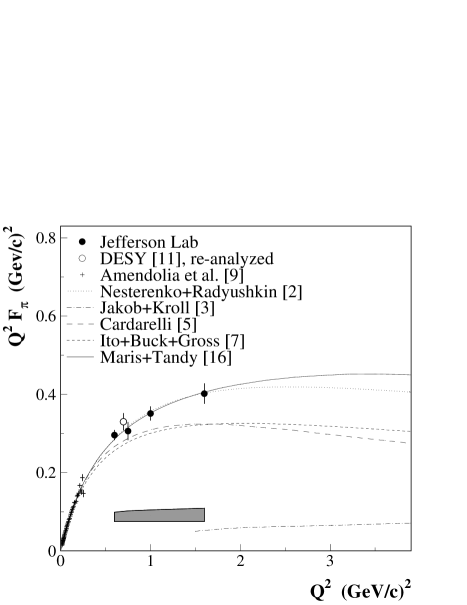
FIG. 3.: The Jefferson Laboratory and reanalyzed DESY values for $F_{\pi}$ in comparison to the results of several calculations. The model uncertainty is represented by the gray area. The (model-independent) data from Ref. [9] are also shown. A monopole behaviour of the form factor obeying the measured charge radius is almost identical to the Maris and Tandy curve.

matical region where the t-pole process is dominant. Values for $F_{\pi}$ were extracted from the longitudinal cross section using a recently developed Regge model. Since the model does not give a perfect description of the $t$-dependence of the data, our results for $F_{\pi}$ contain a sizeable model uncertainty. Improvements in the theoretical description of the ¹H$(e,e^{\prime}\pi^{+})n$ reaction hopefully will reduce those. The data globally follow a monopole form obeying the pion charge radius, and are well above values predicted by pQCD calculations.

The authors would like to thank Drs. Guidal, Laget and Vanderhaeghen for stimulating discussions and for making their computer program available to us. This work is supported by DOE and NSF (USA), FOM (Netherlands), NSERC (Canada), KOSEF (South Korea), and NATO.

REFERENCES

- [1] H.-N. Li and G. Sterman, Nucl. Phys. B381 (1992) 129
- [2] V. A. Nesterenko and A. V. Radyushkin, Phys. Lett. B115 (1982) 410; A.V. Radyushkin, Nucl. Phys. A532 (1991) 141
- [3] R. Jakob and P. Kroll, Phys. Lett. B315 (1993) 463
- [4] V.M. Braun, A. Khodjamirian and M. Maul, Phys. Rev. D 61 (2000) 073004
- [5] F. Cardarelli et al., Phys. Lett. B332 (1994) 1; Phys. Lett. B357 (1995) 267
- [6] N.G. Stefanis, W. Schroers and H.-Ch. Kim, Phys. Lett. B449 (1999) 299 and hep-ph/0005218
- [7] H. Ito, W. W. Buck and F. Gross, Phys. Rev. C 45 (1992) 1918
- [8] P. Maris and C. D. Roberts, Phys. Rev. C 58 (1998) 3659
- [9] S. R. Amendolia et al., Nucl. Phys. B277 (1986) 168
- [10] C. J. Bebek et al., Phys. Rev. D 17 (1978) 1693
- [11] P. Brauel et al., Z. Phys. C3 (1979) 101
- [12] J. Volmer, PhD thesis, Vrije Universiteit, Amsterdam (2000), unpublished
- [13] P. E. Bosted, Phys. Rev. C 51 (1995) 409
- [14] M. Vanderhaeghen, M. Guidal and J.-M. Laget, Phys. Rev. C 57 (1998) 1454; Nucl. Phys. A627 (1997) 645
- [15] F. Gutbrod and G. Kramer, Nucl. Phys. B49 (1972) 461
- [16] P. Maris and P. C. Tandy, preprint nucl-th/0005015