Crossing the dripline to ¹¹N using elastic resonance scattering

Abstract

The level structure of the unbound nucleus ¹¹N has been studied by ¹⁰C+p elastic resonance scattering in inverse geometry with the LISE3 spectrometer at GANIL, using a ¹⁰C beam with an energy of 9.0 MeV/u. An additional measurement was done at the A1200 spectrometer at MSU. The excitation function above the ¹⁰C+p threshold has been determined up to 5 MeV. A potential-model analysis revealed three resonance states at energies 1.27${}^{+0.18}_{-0.05}$ MeV ($\Gamma$=1.44$\pm$0.2 MeV), 2.01${}^{+0.15}_{-0.05}$ MeV, ($\Gamma$=0.84$\pm$0.2 MeV) and 3.75$\pm$0.05 MeV, ($\Gamma$=0.60$\pm$ 0.05 MeV) with the spin-parity assignments I^π=1/2⁺, 1/2^-, 5/2⁺, respectively. Hence, ¹¹N is shown to have a ground state parity inversion completely analogous to its mirror partner, ¹¹Be. A narrow resonance in the excitation function at 4.33$\pm$0.05 MeV was also observed and assigned spin-parity 3/2^-.

PACS number(s): 21.10.Hw, 21.10.Pc, 25.40.Ny, 27.20.+n

]

I Introduction

The exploration of exotic nuclei is one of the most intriguing and fastest expanding fields in modern nuclear physics. The research in this domain has introduced many new and unexpected phenomena of which a few examples are halo systems, intruder states, soft excitation modes and rare $\beta$-delayed particle decays. To comprehend the new features of the nuclear world that are revealed as the drip-lines are approached, reliable and unambiguous experimental data are needed. Presently available data for nuclei close to the driplines mainly give ground-state properties as masses, ground state $I^{\pi}$ and beta-decay half-lives. Also information on energies, widths and quantum numbers $I^{\pi}$ of excited nuclear levels are vital for an understanding of the exotic nuclei but are to a large extent limited to what can be extracted from $\beta$ decays. Nuclear reactions can give additional information, in particular concerning unbound nuclear systems. However, the exotic species are mainly produced in complicated reactions between stable nuclei. These processes are normally far too complex to allow for spin-parity assignments of the populated states, and hence are of limited use for spectroscopic investigations. Instead of using complex reactions between stable nuclei, the driplines can be approached in simple reactions involving radioactive nuclei. An example is given in this paper where elastic resonance scattering of a ¹⁰C beam on a hydrogen target was used to study the unbound nucleus ¹¹N. With heavy ions as beam and light particles as target, the technique employed here is performed in inverse geometry. The use of a thick gas target instead of a solid target is another novel approach. This technique has been developed at the Kurchatov Institute [1] where it has been employed to study unbound cluster states with stable beams [2]. The perspectives of using radioactive beams in inverse kinematics reactions to study exotic nuclei are discussed in [3] and the method was used in [4]. Resonance elastic scattering in inverse kinematics using radioactive beams and a solid target has been used at Louvain-la-Neuve [5, 6].

This experiment is part of a large program for investigating the properties of halo states in nuclei [7]. A well studied halo nucleus is ¹¹Be where experiments have demonstrated that the ground state halo mainly consists of an $1s_{1/2}$ neutron coupled to the deformed ¹⁰Be core [8, 9], in contradiction to shell-model which predicts that the odd neutron should be in a $0p_{1/2}$ state. The $0p_{1/2}$ level is in reality the first excited state, while the ground state is a $1s_{1/2}$ intruder level [10]. This discovery has been followed by numerous papers investigating the inversion, e. g. references [11, 12]. The mirror nucleus of ¹¹Be, ¹¹N, should have a 1/2⁺ ground state with the odd proton being mainly in the $1s_{1/2}$ orbit, if the symmetry of mirror pairs holds. However, ¹¹N is unbound with respect to proton emission which means that all states are resonances that can be studied in elastic scattering reactions. The first experiment devoted to a study of the properties of the low-energy structure of ¹¹N used the three-nucleon transfer-reaction ¹⁴N(³He,⁶He)¹¹N. The results indicated a resonant state at 2.24 MeV [13] which was interpreted as the first excited 1/2^- state rather than the 1/2⁺ ground state.

In this paper we present excitation functions at laboratory (lab.) angles of 0^∘ measured at GANIL [4] and MSU, and at 12.5^∘ with respect to the beam direction measured at GANIL. A thorough analysis, using a potential model as well as a simplified R-matrix treatment, gives unambiguous determination of the quantum structure of the three lowest resonances in the ¹⁰C+p system.

II Elastic resonance scattering: method and formalism

The first description of elastic resonance scattering was given by Breit and Wigner [14], and it is now a theoretically well understood reaction mechanism [15, 16]. Traditionally, elastic resonance scattering experiments have been performed by bombarding a thin target with a light ion beam, narrow in space and time. To obtain an excitation function the beam energy then had to be changed in small steps of the order of the experimental resolution. The need for a radioactive target severely limits the applicability of this method to investigations in regions close to $\beta$ stability. However, it is possible to produce dripline species in simple reactions involving radioactive nuclei. When using this approach, the beam is composed of radioactive ions and the target of light nuclei, eliminating the need for a radioactive target. Since this is the inverse setup to the one traditionally used in scattering experiments, the method is usually denoted as elastic scattering in inverse geometry.

The advantage of using gas instead of a solid target is twofold. Firstly, the thickness of a gas target can be changed continuously and easily by adjusting the gas pressure, and secondly the target is very homogeneous. The beam parameters of radioactive ion beams (RIB’s) are limited; the spread in both energy and space are much larger than what can be obtained for stable beams, and the intensities are of course much smaller. As will be seen below, the beam properties are not of great importance in the experimental approach used here. Elastic resonance scattering is characterized by large cross sections and is therefore well suited for use with low-intensity RIB’s. These and several other features of the elastic resonance scattering in inverse geometry on thick targets will be illuminated in the following subsections.

The expressions for elastic cross section in the case of proton scattering on spin-less nuclei, eqs. 1 and 2, can for example be found in [16],

$$\frac{d\sigma}{d\Omega}=\left|A(\theta)\right|^{2}+\left|B(\theta)\right|^{2},$$ (1)

where

$$\begin{split}A(\theta)=\frac{zZ}{2\mu v\sin^{2}(\theta/2)}e^{\frac{i\hbar}{\mu v}\ln\frac{1}{\sin^{2}(\theta/2)}}+\\ \frac{1}{2ik}\sum_{\ell=0}^{\infty}\left[(\ell+1)(e^{2i\delta^{+}_{\ell}}-1)+\ell(e^{2i\delta^{-}_{\ell}}-1)\right]\\ e^{2i\sigma_{\ell}}P_{\ell}(\cos\theta)\end{split}$$ (2)

and

$$B(\theta)=\frac{i}{2k}\sum_{\ell=0}^{\infty}\left(e^{2i\delta^{+}_{\ell}}-e^{2i\delta^{-}_{\ell}}\right)e^{2i\sigma_{\ell}}P^{1}_{\ell}(\cos\theta)$$ (3)

where $e^{2i\sigma_{\ell}}$ is defined by

$$e^{2i\sigma_{\ell}}=\frac{\Gamma\left(\ell+1+\frac{i}{k}\right)}{\Gamma\left(\ell+1-\frac{i}{k}\right)}$$ (4)

Symbols introduced here are defined as: ^±: denotes states with $j$ = $\ell\pm\frac{1}{2}$ $z$: charge of the proton $Z$: charge of the spin-zero particle $\mu$: reduced mass $v$: the relative velocity of the particles $k$: the magnitude of the wave vector $\sigma_{\ell}$: the Coulomb phase shift $P_{\ell}(cos\theta)$: Legendre polynomial $P^{1}_{\ell}(cos\theta)$: associated Legendre polynomial

The first term in $A(\theta)$ represents the Coulomb scattering. The other terms in $A(\theta)$ and $B(\theta)$ express scattering due to nuclear forces. The phase shift $\delta_{\ell}$ is the sum of the phase shift from hard sphere scattering, $-\phi_{\ell}$, and the resonant nuclear phase shift, $\beta_{\ell}$,:

$$\delta^{+}_{\ell}=\beta^{+}_{\ell}-\phi_{\ell},\quad\delta^{-}_{\ell}=\beta^{-}_{\ell}-\phi_{\ell}$$ (5)

The differential cross-section has its maximum in the vicinity of the position where the phase shift passes through $(n+\frac{1}{2})\pi$. Therefore, a frequently used definition of the resonance energy is where $\delta$ = $(n+\frac{1}{2})\pi$, see section IV. It is favourable to study resonance scattering at 180^∘ c.m. where eq. 1 is simplified. At this angle, only $m=0$ sub-states contribute to the cross section and both potential and Coulomb scattering are minimal. An advantage of the inverse geometry setup is its possibility to measure at 180^∘ c.m.

A Kinematical relations

We define the laboratory energies of the bombarding particles before the interaction in inverse (E) and conventional (T) geometry as $E_{0}$ and $T_{0}$, respectively. The notation used mainly follows ref. [17], primed energies being in the c.m. system:

$m$,$M$: mass of the light and heavy particles $E_{M}$, $T_{M}$: heavy particle $M$ laboratory energies after interaction $E_{m}$, $T_{m}$: light particle $m$ laboratory energies after interaction $\theta_{lab.}$: scattering angle of the light particle in the laboratory system

The relations between laboratory energy of the beam and the c.m. energy of the heavy nucleus:

$${T_{M}^{{}^{\prime}}}=T_{0}\frac{mM}{\left({M}+m\right)^{2}}\Leftrightarrow{E_{M}^{{}^{\prime}}}={E_{0}\left(\frac{m}{{M}+m}\right)^{2}}$$ (6)

The expressions for the lab. energies of the light particle $m$ that will be detected after scattering:

$$\begin{split}{T_{m}}={T_{0}}\Big{(}\frac{m}{{M}+m}\Big{)}^{2}\big{(}\cos{\theta_{lab.}}+\sqrt{K^{2}-\sin^{2}{\theta}}\big{)}^{2}\\ \Leftrightarrow{E_{m}}={E_{0}}\frac{4mM}{({M}+m)^{2}}\cos^{2}\theta_{lab.}\end{split}$$ (7)

In the equation above, $K$ is the ratio of the masses ($E_{0}$/$T_{0}$=$M/m=K$ since ${E_{M}^{{}^{\prime}}}={T_{M}^{{}^{\prime}}}$). Inserting $\theta_{lab.}=0^{\circ}$ in eq. 7 leads to the following ratio between the energy of the measured particle in conventional and inverse geometry:

$$\frac{E_{m}}{T_{m}}=4\frac{K^{2}}{(1+K)^{2}}\sim 4$$ (8)

As is seen from eq. 8, the detected energy of the light particles is close to 4 times higher for inverse kinematics as compared to the conventional geometry at the same c.m. energy. This is an important gain for the study of resonant states near the threshold. The excitation energy in the ${M}+m$ compound system is obtained as the sum of the c.m. energies for particles $m$ and $M$:

$$\begin{split}{T_{ex}}={T_{0}}\frac{M}{{M}+m}\Leftrightarrow{E_{ex}}={E_{0}}\frac{m}{{M}+m}\end{split}$$ (9)

Using eq. 7, this can be expressed in terms of the measured particle energy $E_{m}$. In case of inverse kinematics, the excitation energy of the compound system becomes:

$$E_{ex}=\frac{{M}+m}{4M\cdot cos^{2}(\theta_{lab.})}E_{m}$$ (10)

Because of the low energies involved, a non-relativistic expression can be used.

B General set-up of elastic scattering in inverse geometry

The basic experimental setup consists of a radioactive ion beam which is incident on a scattering chamber filled with gas. The thickness of the gas target is adjusted to be slightly greater than the range of the beam ions. Charged-particle detectors are placed at and around the beam direction, i.e. 180^∘ c.m., as shown in Figure 1. As they are continuously slowed down in the gas, the beam ions effectively scan the energy region from the beam energy down to zero, giving a continuous excitation function in this interval. When the energy of the heavy ion corresponds to a resonance in the compound system, the cross section for elastic scattering increases dramatically and can exceed 1 b, making it possible to neglect the non-resonant contributions which are on the order of mb. For the ideal case of a mono-energetic beam, each interaction point along the beam direction in the chamber corresponds uniquely to one resonance energy and, as we study elastic scattering, to a specific proton energy for each given angle. Because the distance from the detector is different for each proton energy, the solid angle also varies with proton energy and is quite different for low and high energy resonances.

The high efficiency of the method is mainly a result of the large investigated energy region. If we compare the scanned region of 5-10 MeV with the typical energy step of $\approx$10-20 keV in conventional scattering measurements, the gain is 250-1000 times.

C Energy resolution

The initial energy spread of our ¹⁰C beam was 1.5% of the total energy, which naturally increased along the beam path in the gas. The energy spread of the beam results in excitation of the same resonance at different distances from the detector. Assuming that ${\Delta}E$ is the energy spread at some point in the gas, this distance interval ${\Delta}x$ is given by

$${\Delta}x=\frac{{\Delta}E}{(\frac{dE}{dx})_{M}}$$ (11)

where $(\frac{dE}{dx})_{M}$ is the specific energy loss of the beam nuclei in the gas. Due to the protons energy loss in the gas, the measured proton energies corresponding to the same resonance are slightly different. The resulting spread of proton energies, ${\varepsilon}$, corresponding to the interval ${\Delta}x$ will be

$$\varepsilon={\Delta}E\frac{(\frac{dE}{dx})_{m}}{(\frac{dE}{dx})_{M}}$$ (12)

Here, $(\frac{dE}{dx})_{m}$ denotes the specific energy loss of the recoil nuclei (protons) in the gas. Taking into account the different velocities of the beam ions and the scattered protons as well as the Bethe-Bloch expression for specific energy loss, one finds:

$${\varepsilon}{\sim}\frac{{\Delta}E}{4}\frac{z^{2}}{Z^{2}}$$ (13)

In the case of ¹⁰C+p interaction, eq. 13 becomes ${\varepsilon}{\sim}\frac{{\Delta}E}{144}$. Hence, for $\Delta$E = 5 MeV a lab. energy resolution of 35 keV is expected. The effective c.m. energy resolution will be about four times better than the resolution in the lab. frame, see eq. 8. Thus it is clearly shown that the energy spread of the radioactive beam does not restrict the applicability of the method. Many other factors influence the final resolution, for example the size of the beam spot and detectors, the detector resolution, the angular divergence of the beam and straggling of light particles in the gas. These factors can be taken into account by Monte Carlo simulations. In reality, an effective energy resolution of 20 keV in the c.m. frame is feasible. At angles other than 180^∘ the resolution deteriorates, mainly due to kinematical broadening of the energy signals for protons scattered at different angles. This contribution to the resolution could be reduced by tracking the proton angles.

D Background sources

A cornerstone of the described experimental approach is that elastic resonance scattering dominates over other possible processes. The competing reaction channel which has to be treated for each specific case is inelastic resonance scattering, as it is a resonant process which produces the same recoil particles as the elastic scattering. However, the elastic and inelastic resonance scattering reactions can be distinguished from each other. The energy of the scattered nuclei from inelastic resonance scattering at 0^∘ is given by eq. 14 if $E^{*}/E_{0}{\ll}$ 1, where $E^{*}$ is the excitation energy of the beam nucleus [17].

$$E_{m}\ {\approx}\ 4\frac{mM}{({M}+m)^{2}}\Big{(}E_{0}-{\frac{E^{*}}{2}}{\frac{{M}+m}{m}}\Big{)}$$ (14)

Comparing this with eq. 10, one sees that the energy of heavy ions has to be larger by an amount $\mathcal{E}$ for the inelastic scattering to obtain the same energy of a light recoil from the elastic and inelastic scattering reactions, when $\mathcal{E}$ is defined in eq. 15 .

$$\mathcal{E}{\approx}\frac{\mathnormal{E}^{*}}{\mathrm{2}}\mathnormal{{\frac{{M}+m}{m}}}$$ (15)

For the ¹⁰C+p case, where $E^{*}$(¹⁰C(2${}^{+}_{1}$)) = 3.35 MeV, eq. 15 shows that the inelastic resonance scattering should take place at about 20 MeV higher energy than the elastic one for the two processes to mix in the elastic scattering excitation function. The inelastic resonance reaction thus has to take place further from the detectors, closer to the entrance window, in order to produce a scattered particle with the same energy as the corresponding elastic process. The two processes in question hence can give the same energies of the recoil protons but their ToF (window-detector) will differ. The time difference between the two types of events will be on the order of a few ns, and can thus be separated in the analysis. No such events were seen in our data.

Other scattering reactions contribute very little to the spectrum, especially at 180^∘ c.m., the exception being low energies where the Coulomb scattering cross sections increases. However, this scattering is well understood and can be included in the data treatment. Additional sources of background are $\beta$ particles from decaying radioactive ions in the gas, beam ions which penetrate the gas target, and particles scattered in the entrance window.

III Experimental procedure

The first experiment was performed using the LISE3 spectrometer at the GANIL heavy-ion facility. The secondary ¹⁰C beam was produced by a 75 MeV/u ¹²C⁶⁺ beam with an intensity of 2$\cdot$10¹² ions/s which bombarded a 8 mm thick, rotating Be target and a fixed 400 $\mu$m Ta target. The ¹⁰C fragments were selected in the LISE3 spectrometer, using an achromatic degrader at the intermediate focal plane (Be, 220 $\mu$m thick) and the Wien-filter after the last dipole. The 50 cm long scattering chamber was placed at the final focal plane. Immediately before the 80 $\mu$m thick kapton entrance window, a PPAC (Parallel Plate Avalanche Counter) registered the position of the incoming ions. The intensity of the secondary beam, measured by the PPAC, was approximately 7000 ions/s, and due to the degrader and Wien filter a very low degree of contamination was achieved. The efficiency of the PPAC at this intensity and ion charge is close to 100%, which makes it easy to use the PPAC count rate to obtain absolute cross-sections. The scattering chamber was filled with CH₄ gas, acting as a thick proton target for the incoming ¹⁰C ions. The gas pressure was adjusted to 816$\pm$5 mbar, which was the pressure required to stop the incoming beam just in front of the central detector. It is desirable to stop the beam close to the detectors in order to avoid loosing any protons scattered from a possible low-lying resonance in ¹¹N. In the far end of the chamber an array of Si-detectors was placed. The detectors had diameters of 20 mm and thickness of 2.50 mm, corresponding to the range of 20 MeV protons. The time between the radio frequency (RF) from the cyclotron and the PPAC gave one time-of-flight signal (ToF), while the time difference of the PPAC and detector signal gave additional ToF-information. The complete setup is shown in Figure 1.

As a first measurement, a low intensity ¹⁰C beam was sent into the evacuated scattering chamber to get the total energy and spread of the secondary beam after the foil, and this was determined to be 90 MeV with a FWHM = 1.5 MeV. For background measurements, the scattering chamber was filled with CO₂ gas at 450$\pm$5 mbar and bombarded with ¹²C and ¹⁰C beams, respectively. For our purposes, we assume that ¹⁶O and ¹²C behave similarly in proton scattering reactions. The measurements with the CO₂ target would reveal any background stemming from the carbon nuclei in the CH₄ target gas or from the kapton window. Beam contaminations would also be present in these runs, and those background sources can subsequently be subtracted from the experimental excitation functions.

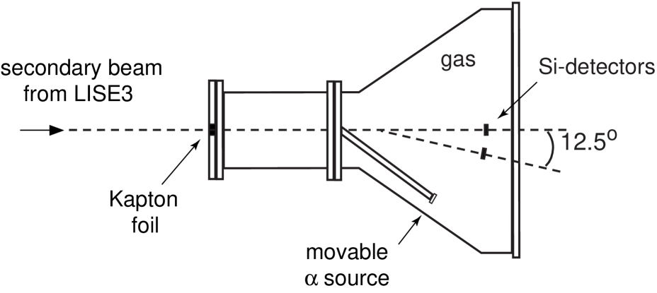
FIG. 1.: A schematic view of the scattering chamber and Si-detectors. The 12.5^∘ detector has this angle to the middle of the chamber. The interaction position and the corresponding angle is calculated for each event when analyzing the data.

The standard beam diagnostics observed admixtures of d, $\alpha$ and ⁶Li with the same velocity as the ¹²C secondary beam, while no contaminant particles could be seen in the ¹⁰C beam. The ¹⁰C+CO₂ spectrum showed no prominent structure and was found to contribute less than 10% to the total cross section. This background spectrum was subtracted from the ¹⁰C+CH₄ spectrum before transformation to the c.m. system.

Since ¹⁰C is a $\beta^{+}$ emitter with a half life of 19.3 s, it is necessary to discriminate the positron signals from the protons. This was done by selecting the protons in a two-dimensional spectrum showing ToF (PPAC to Si-detector) versus detected energy, where the positrons are clearly distinguished from protons both by their uniform time distribution and their maximum energy of 1.93 MeV. A positron with energy in this interval has a maximum energy loss of 1.25 MeV in 2.50 mm Si, which simulates a scattered proton energy of 0.344 MeV in the excitation function of ¹¹N. Since the positron energies are small enough to lie in the energy range of Coulomb scattered protons, cutting away all events below this energy does not distort the interesting parts of the proton spectrum, as is seen in the inset in Figure 3.

In this paragraph we justify our ignoring the background contributions to our spectra from inelastic scattering of ¹⁰C on hydrogen with excitation of the particle stable 2⁺ level at 3.35 MeV in ¹⁰C. The contribution from inelastic scattering has been estimated using available data on inelastic scattering of protons on a ¹⁰Be target [18] and a DWBA extrapolation to the whole investigated interval of energies. This shows that the contribution from inelastic scattering does not exceed 1% of the observed cross section.

The energy calibration of the Si detectors was done with a triple $\alpha$-source (²⁴⁴Cm, ²⁴¹Am and ²³⁹Pu) which was placed on a movable arm inside the chamber. Another calibration, and at the same time a performance check of the setup, was done by investigating known resonances in ¹³N. The primary ¹²C beam, degraded to 6.25 MeV/u, was scattered on the methane target using a gas pressure of 240$\pm$5 mbar. The resulting proton spectrum clearly shows the two closely lying resonances in ¹³N (3.50 MeV, width 62 keV, and 3.55 MeV, width 47 keV, [19]), as can be seen in Figure 2.

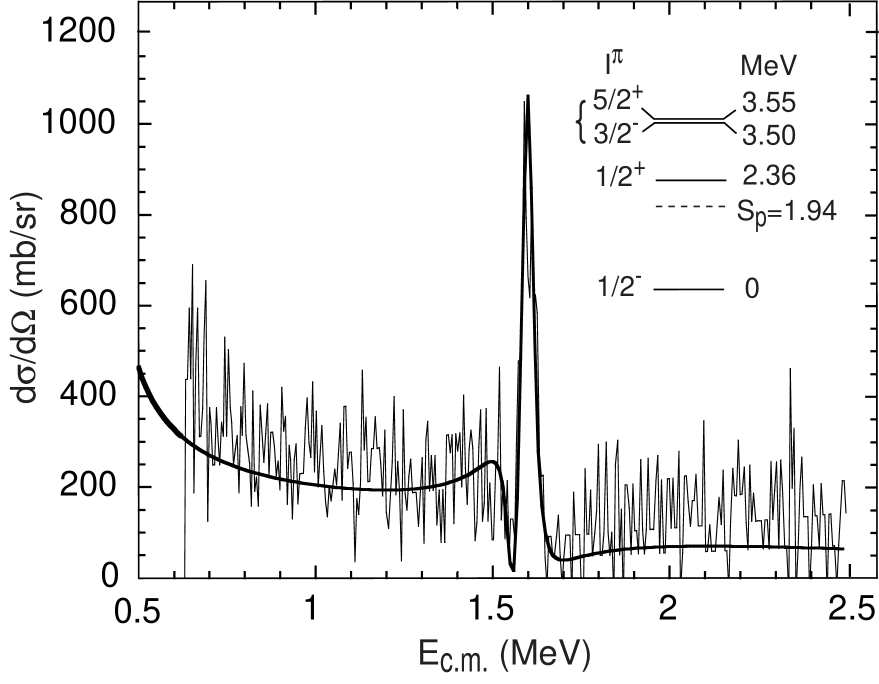
FIG. 2.: Experimental spectrum of protons from the scattering of ¹²C. The energy is given as c.m. energy of ¹³N. The peaks are fitted with two coherently added resonances as described in the text.

These resonances are overlapping and the width of the peak is 50 keV. The solid curve in Figure 2 is a fit obtained by coherently adding two curves in order to take interference into account. The 5/2⁺ resonance at 3.55 MeV has single particle (SP) nature [19] and was described using the potential model outlined in section IV, while a Breit-Wigner curve was used for the 3/2^- state at 3.50 MeV. The resonant 1/2⁺ state in ¹³N, 420 keV above the ¹²C+p threshold, is not seen as it is overlapping the Coulomb scattering which dominates below 0.5 MeV. From the calibration measurements described above an energy resolution of 100 keV in the lab. frame was deduced, mainly determined by the detector resolutions and proton straggling in the gas.

The experimental proton spectrum was, after subtraction of the measured carbon background, transformed into differential cross-section as a function of the excitation energy of ¹¹N, in the following referred to as the excitation function of ¹¹N. Since each interaction point along the beam direction ideally corresponds to a specific resonance energy, the measured proton energy can, after correction for its energy loss in the gas, be used to find the resonance energy in ¹¹N in the c.m. system. The inset in Figure 3 shows the experimental data as measured proton energy versus counts at 0^∘ before the corrections for solid angle was made. Comparing this pictures to the one obtained after transformation to the c.m. system clearly shows the effect of differing solid angles for different proton energies. The cross sections in the high energy part increases relative to the low energy part, as is clearly seen when comparing the inset to the transformed spectrum in Figure 3.

Extracting the cross section from the data is straightforward, and the transformation to c.m. is done using eq. 16.

$$\Big{(}\frac{d\sigma}{d\Omega}\Big{)}_{c.m.}=\frac{1}{4cos(\theta_{lab.})}\Big{(}\frac{d\sigma}{d\Omega}\Big{)}_{lab.}$$ (16)

The relation between the scattering angle in the lab. and c.m. systems is simply $\theta_{c.m.}$=180^∘-2$\theta_{lab.}$. The excitation function obtained after background subtraction and transformation into the c.m. system is shown in Figure 3.

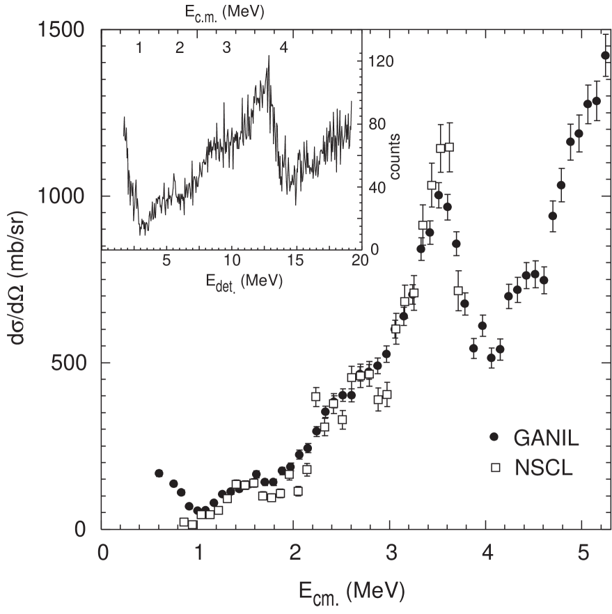
FIG. 3.: The excitation function of ¹¹N is shown after background subtraction and transformation to the c.m. system. The filled black circles represent the GANIL data, and the white squares show the result of the MSU experiment. The inset shows the raw data in the lab. system. The upper scale in the inset is a rough calibration to c.m. energy, shown for comparison, while the lower scale is the detected proton energy.

The more detailed analysis now performed revises the absolute cross section to a larger value from what was previously published in [4].

A second independent measurement of ¹⁰C+p elastic scattering using the same method was made at NSCL where the A1200 spectrometer delivered the ¹⁰C beam. The experimental conditions were the same as in the GANIL experiment, except that at NSCL a $\Delta$E-E telescope was placed at 0^∘ and no Wien-filter was used. The energy of the ¹⁰C beam after the foil was 7.4 MeV/u and the beam intensity was 2000 pps. The data from these two experiments are overlaid in Figure 3 where it is seen that the structures and the absolute cross sections coincide.

IV Analysis and results

The excitation function, shown in Figure 3, reveals structure in the region from 1 MeV to 4 MeV that could be due to interfering broad resonances. A reasonable first assumption is that the structure corresponds to the three lowest states in ¹¹N. This assumption is justified by the closed proton $p_{3/2}$ sub-shell in ¹⁰C and agrees with the known predominantly single particle nature of the lowest states in ¹¹Be [20], the mirror nucleus of ¹¹N. Taking this as a starting point, we assume that the observed levels in ¹¹N are mainly of SP nature. The SP assumption validates the use of a shell-model potential to describe the experimental data of ¹¹N.

A Analysis of the three lowest levels in ¹¹N

The ¹¹N states are all in the continuum and the aim of the analysis was to obtain $I^{\pi}$ and other resonance parameters as it can be done in the framework of the optical model. Because of the absence of other scattering processes than the elastic scattering channel, no imaginary part is included in the potential. The potential has a common form consisting of a Woods-Saxon central potential and a spin-orbit term with the form of a derivative of a Woods-Saxon potential. The Woods-Saxon ($\ell$s) term has the usual parameters $V_{0}$ ($V_{{\ell}s}$), $r_{0}$ ($r_{{\ell}s}$) and $a_{0}$ ($a_{{\ell}s}$) for well depth, radius and diffusity, respectively. Centrifugal and Coulomb terms were also included in the potential. The Coulomb term has the shape of a uniformly charged sphere with radius $r_{c}$. The full potential is given in eq. 17, where $\mu$ is the reduced mass of the system and $\lambda_{\pi}$ denotes the pion Compton wavelength.

$$\begin{split}V_{0}=\frac{V_{\ell}}{1+e^{\frac{r-R_{0}}{a_{0}}}}+{\bf\ell\cdot s}\frac{V_{\ell s}(\lambda_{\pi}/2\pi)^{2}}{a_{\ell s}}\times\\ \frac{e^{\frac{r-R_{\ell s}}{a_{\ell s}}}}{\left(1+e^{\frac{r-R_{\ell s}}{a_{\ell s}}}\right)^{2}}+\quad\frac{\ell(\ell+1)\hbar^{2}}{2{\mu}r^{2}}+V_{c}\end{split}$$ (17)

$$V_{c} = \begin{cases}\frac{zZ}{2}\frac{e^{2}}{4{\pi}{\epsilon_{0}}R_{c}}\left(3-\frac{r^{2}}{R_{c}^{2}}\right)&:\quad r<R_{c}\\ \frac{zZe^{2}}{r}&:\quad r>R_{c}\end{cases}$$ (18)

$$R_{0}=r_{0}A^{1/3},\ R_{c}=r_{c}A^{1/3},\ R_{\ell s}=r_{0}A^{1/3}$$ (19)

As a starting point, standard values of the potential parameters were chosen [21] and the well depths were varied separately for each partial wave ($\ell$=0,1,2), see Table I:a. The cross-section of the experimental data at 180^∘ was found to be larger than predicted by the potential model. As can be seen in the experimental spectrum, Figure 3, there is substantial amount of cross section above 4 MeV, indicating additional resonances in this energy region.

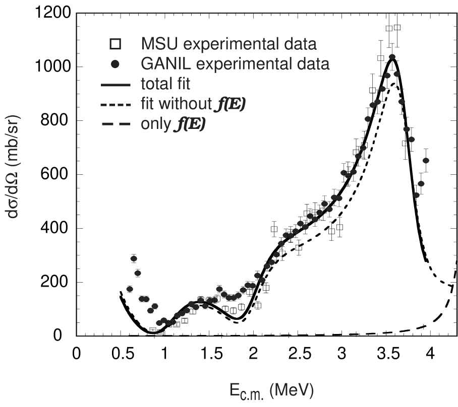
FIG. 4.: Experimental excitation function of ¹¹N together with the best fit from the SP-model program. The energy is given as excitation energy of ¹¹N. The fit is made using a potential with parameters shown in Table I:c. The underestimation of the cross section around 1.8 MeV is the only failure of the potential model. This part is better described when the influence of higher resonances are taken into account, see Figure 9.

The underestimation of the potential model can thus be attributed to influence of higher lying resonances. To simulate the presence of those highly excited states, an amplitude $f$ was added to the amplitude calculated from the potential model. The form of this extra amplitude was $f=\frac{b}{E_{0}-E}$, where $E_{0}$ was taken as a constant (4.5 MeV) and $b$ was used as a parameter. As is seen in Figure 4, the introduced amplitude is small in comparison with the measured cross sections, but it nonetheless was useful in the fitting procedure. A more sophisticated way to include the influence of higher resonances is to use an R-matrix procedure, and some attempts in this way were also made, see sec. IV B.

The best fit for conventional parameter values, only varying $V_{\ell}$ is obtained for the level ordering $1s_{1/2}$, $0p_{1/2}$, and $0d_{5/2}$, and the corresponding parameters are given in Table I:a. The curve resulting from these parameters does not differ significantly from the one obtained using the parameter set Table I:c.

A potential with conventional parameters and the same well depth for all $\ell$ will generate single particle levels in the order $0p_{1/2}$, $1s_{1/2}$ and $0d_{5/2}$ above the $0p_{3/2}$ sub-shell. However, all attempts to describe the experimental data keeping this ordering of the levels failed. A typical example of a calculated excitation function with this level sequence is shown in Figure 5, with parameters in Table I:b. This result is not surprising when considering the well known level inversion in ¹¹Be.

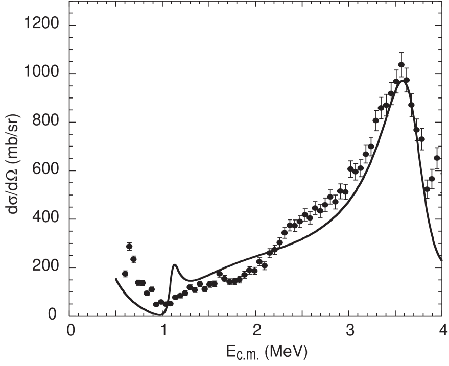
FIG. 5.: A typical fit of the experimental data when the 1/2^- state is assumed to be the ground state of ¹¹N. It is evident that the excitation function is not well described. Putting the $p$ state this low makes it too narrow, at the same time as the $s$ state becomes very broad since it is now well above the Coulomb barrier.

For the potential in Table I:c, the cross section of each partial wave is shown in Figure 6 together with the total calculated curve. Comparing the partial cross sections with the total cross section, it is clear that interference between the partial waves determine the shape of the total curve. The corresponding phase shifts are shown in Figure 7. The most common definition of resonance energy is where the phase shift $\delta_{\ell}$ passes $\pi$/2. As is seen in Figure 7, the phase of the 1/2⁺ resonance, which is the broadest level, does not reach $\pi$/2. Therefore, we have defined the resonance energy as where the partial-wave amplitude calculated at r = 1 fm has its maximum. The width is defined as the FWHM of the partial wave. One can note that for the 1/2^- and 5/2⁺ levels, the same resonance energies are obtained by our definition and $\delta_{\ell}$ = $\pi$/2. All attempts to change the resonance spins and parities or the order of the levels resulted in obvious disagreement with the experimental data. We thus conclude that the unambiguous spin-parity assignments for the lowest states in ¹¹N are a 1/2⁺ ground state, a first excited 1/2^- level and a 5/2⁺ second excited state. All further fitting procedures were performed with the aim to obtain more exact data on the positions and widths of the resonances.

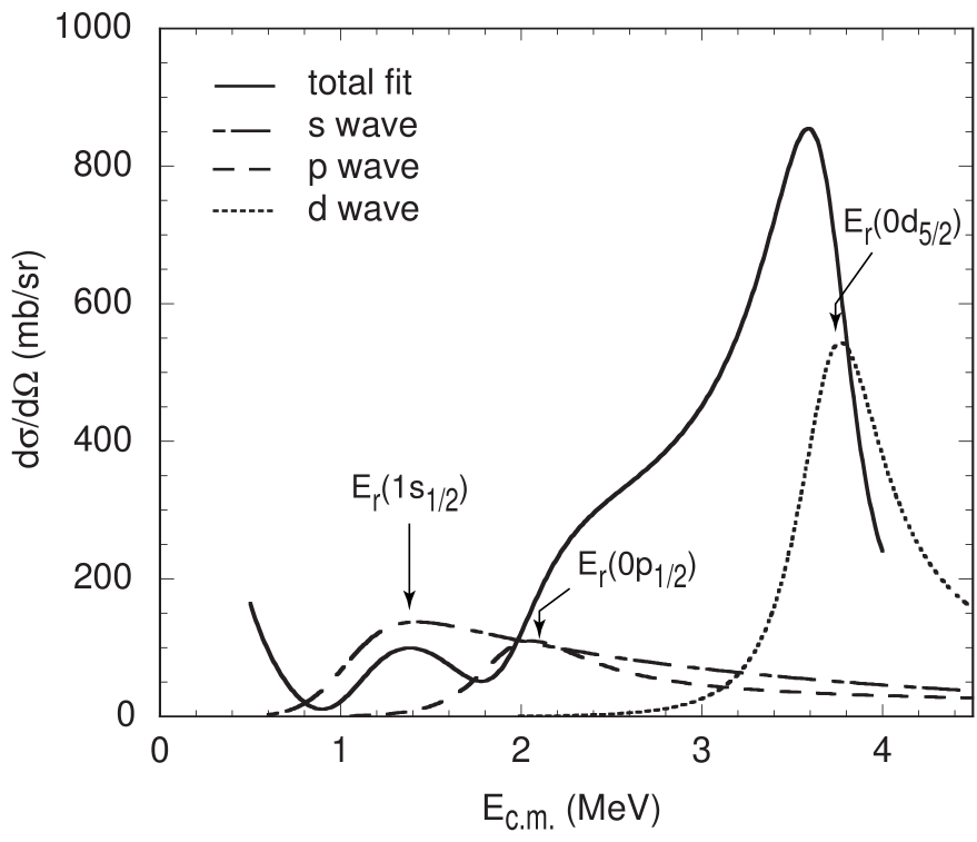
FIG. 6.: The partial waves $s_{1/2}$, $p_{1/2}$ and $d_{5/2}$ together with the total calculated excitation function for the best fit to the experimental data (Table I:c).

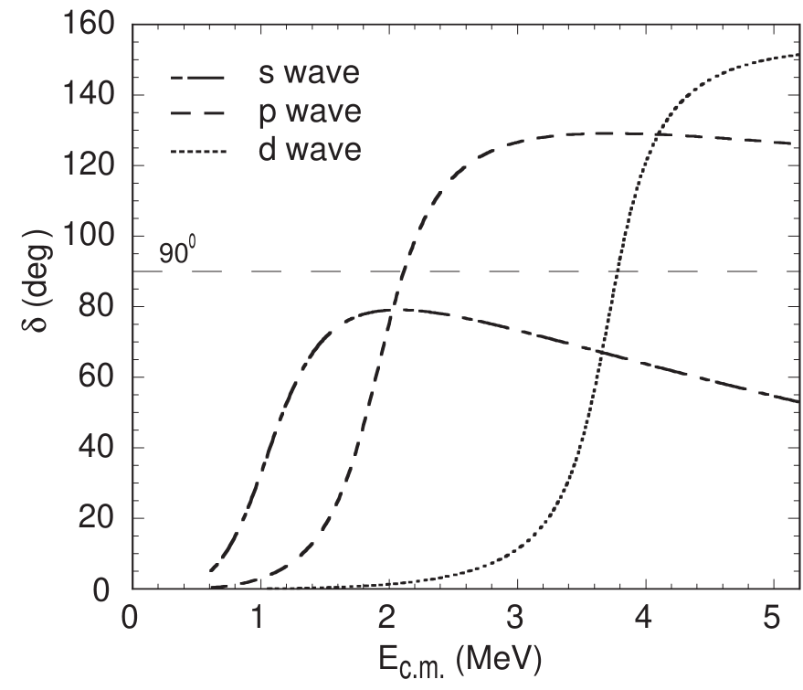
FIG. 7.: The phase shifts from the theoretically calculated curve which is the best fit to the experimental data (Table I:c).

A disadvantage of the potential model is that it produces resonances with single-particle widths. In general, the nature of the states is more complicated and their widths can be smaller than what is predicted by the potential model. To investigate how changing the resonance widths would affect the overall fit, we changed the radius parameter $r_{0}$, and fitted new well depths to get the best possible agreement with the data. It was evident that the widths obtained with $r_{0}$ = 1.4 fm are too large for the 1/2^- and 5/2⁺ resonances, while $r_{0}$ = 1.0 fm makes these levels too narrow.

TABLE I.: The sets of potential parameters used to obtain the best fits of the experimental data, and the resulting resonance parameters. $V_{\ell s}$=5.5 MeV is kept the same in all fits. The change of this parameter gave only minor modifications. The parameter $b$ given in the footnotes is the value used in $f(E)$=b/(4.5-E).

		Potential parameters				Resonance
		$V_{\ell}$	$r_{0}$, $r_{\ell s}$, $r_{c}$	$a_{0}$	$a_{\ell s}$	$E_{r}$	$\Gamma_{r}$
		(MeV)	(fm)	(fm)	(fm)	(MeV)	(MeV)
a	$1s_{1/2}$	-66.066	1.20	0.53	0.53	1.30	1.24
	$0p_{1/2}$	-42.336	1.20	0.53	0.53	1.96	0.65
	$0p_{3/2}$	-42.084	1.20	0.53	0.53	-1.06	-
	$0d_{3/2}$	-78.792	1.20	0.53	0.53	4.40	0.90
	$0d_{5/2}$	-64.092	1.20	0.53	0.53	3.72	0.61
b	$1s_{1/2}$	-45.360	1.40	0.65	0.30	1.70	3.49
	$0p_{1/2}$	-33.474	1.40	0.28	0.30	1.11	0.11
	$0p_{3/2}$	-32.340	1.40	0.53	0.30	-1.22	-
	$0d_{3/2}$	-58.086	1.40	0.53	0.30	4.45	1.23
	$0d_{5/2}$	-45.570	1.40	0.35	0.30	3.75	0.60
c	$1s_{1/2}$	-47.544	1.40	0.65	0.30	1.27	1.44
	$0p_{1/2}$	-31.500	1.40	0.55	0.30	2.01	0.84
	$0p_{3/2}$	-32.592	1.40	0.53	0.30	-1.33	-
	$0d_{3/2}$	-57.960	1.40	0.53	0.30	4.5	1.27
	$0d_{5/2}$	-45.570	1.40	0.35	0.30	3.75	0.60
d	$1s_{1/2}$	-56.280	1.20	0.75	0.30	1.32	1.76
	$0p_{1/2}$	-42.420	1.20	0.55	0.30	2.14	0.88
	$0p_{3/2}$	-42.210	1.20	0.53	0.30	-1.33	-
	$0d_{3/2}$	-78.960	1.20	0.53	0.30	5.0	1.39
	$0d_{5/2}$	-62.874	1.20	0.50	0.30	3.79	0.59
e	$1s_{1/2}$	-66.066	1.20	0.53	0.53	1.30	1.24
	$0p_{1/2}$	-42.084	1.20	0.53	0.53	2.04	0.72
	$0p_{3/2}$	-42.084	1.20	0.53	0.53	-1.06	-
	$0d_{3/2}$	-64.092	1.20	0.53	0.53	9.87	4.53
	$0d_{5/2}$	-64.092	1.20	0.53	0.53	3.72	0.61
f	$1s_{1/2}$	-46.074	1.40	0.70	0.30	1.27	1.56
	$0p_{1/2}$	-30.492	1.40	0.70	0.30	2.01	1.09
	$0p_{3/2}$	-32.550	1.40	0.53	0.30	-1.31	-
	$0d_{3/2}$	-57.960	1.40	0.53	0.30	4.50	1.27
	$0d_{5/2}$	-42.378	1.40	0.70	0.30	3.75	1.08
a $r_{0}$=1.2 fm, only varying $V_{\ell}$ (b=1.25)
b No level inversion (b=1.25)
c $r_{0}$=1.4 fm, varying $a$ and $V_{\ell}$ (b=1.25):
the best fit to the data
d $r_{0}$=1.2 fm, varying $a$ and $V_{\ell}$ (b=2.4)
e The parameters used in [4] (b=0)
f The parameters used to obtain the widths in
the single particle limit.

As the 1/2⁺ state is least affected by the change of radius the conclusion for this level is difficult, but the largest obtained width seemed most appropriate. Therefore, the radii parameters $r_{0}$, $r_{{\ell}s}$ and $r_{c}$ were chosen as 1.4 fm, and the well depths and diffusities were varied separately for each $\ell$ to obtain the best fit of the experimental data up to 4 MeV. An additional argument for choosing the larger radius was the fact that this parameter value gives a good simultaneous description of the mirror pair ¹¹Be and ¹¹N [4]. The curve obtained in this way that agreed best with the experimental excitation function is shown in Figure 4, and the corresponding potential parameters and resonance energies and widths are shown in Table I:c. For comparison, the values for $r_{0}$=$r_{{\ell}s}$=$r_{c}$=1.2 fm are also given in Table I:d.

The extracted resonance parameters show a remarkable stability against changes in the potential parameter sets, meaning that different sets of parameters that fit the data give similar resonance energies and widths. This is seen in Table I, comparing different sets of parameters. The final energies and widths are listed in table IV. The error bars include systematic errors and are dominated by a contribution from the spread in results from different parameter sets. Contributions from background subtraction and solid angle corrections will be much smaller than those sources.

The SP reduced widths could be extracted for the three lowest levels where the only possible decay channel is one-proton emission to the ground state of ¹⁰C. The values of reduced widths are usually presented as a ratio to the Wigner limit, which serves as a measure of the single particle width [14]. In our case we have a way to give a more exact evaluation of the reduced widths as the ratio of the widths obtained from the shell-model potential that fits the data (Table I:c) to the widths calculated from a true shell-model potential. These ratios are free from the uncertainties related with different definitions of the level widths.

Since the true shell model potential is not known for ¹¹N, and we approximated this potential with the parameters shown in Table I:f.

TABLE II.: Reduced widths for the observed states obtained from the ratio of the widths from parameter sets c (experimental widths) and f (single particle widths) in Table I.

Level Iπ	Reduced width $\Gamma_{exp}$/$\Gamma_{SP}$
1/2+	0.92$\pm$0.2
1/2-	0.77$\pm$0.2
5/2+	0.56$\pm$0.2
3/2-	0.15$\pm$0.2

Justification for using this particular set as shell model potential is that it simultaneously reproduces the level positions in both ¹¹Be and ¹¹N and gives a width of the 1/2⁺ state that is larger than for the parameters in Table I:c. The reduced widths obtained in this way are given in Table II.

The potential parameters for the fit of the data at 180^∘ (parameter set c in I) were used to describe the excitation function obtained by a detector at 12.5^∘ relative to the center of the chamber. The experimental data from this case are shown in Figure 8 together with the theoretical curve without the scaling amplitude $f$. Comparing the experimental excitation functions in Figures 4 and 8, rather big differences are seen.

This reflects the fact that the laboratory angle depends on the interaction point in the chamber. The angular range goes from $\theta_{c.m.}$=150^∘ for protons from higher resonances to $\theta_{c.m.}$=93^∘ for low energy protons. This is taken into account in the calculation of the excitation function, and from Figure 8 it is evident that the potential model describe the observed changes in the excitation function with angle, a fact which supports our interpretation.

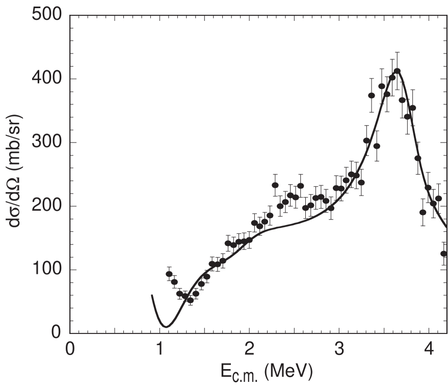
FIG. 8.: Experimental spectrum of protons in the detector placed at 12.5^∘ relative to the center of the chamber. The full drawn curve is the result from the potential model using the parameters given in Table I:c.

B Analysis of the full excitation function

In an attempt to investigate the influence of higher lying states on the cross section in the lower part of the experimental spectrum, a simplified R-matrix approach was used. For ¹¹Be, about 10 levels are predicted in the energy region 2.7 MeV to 5.5 MeV [22], but only four resonances have been experimentally found [20]. The knowledge of the levels in ¹¹N is even more incomplete, and our experimental data are not sufficient for a detailed R-matrix analysis. Therefore, the treatment described below was performed rather to outline possible questions than to give definite answers. The analysis was made using the potential model and adding resonances at energies above 4 MeV according to eq. 20.

$$\begin{split}\frac{d\sigma}{d\Omega}\bigg{(}\theta=180^{\circ}\bigg{)}=\\ \Bigg{|}A_{pot}-\frac{i}{2k}\sum_{n_{\ell}}^{+}\bigg{[}({\ell}+1)\ \left(e^{2i\beta_{\ell}^{+}}-1\right)\ e^{2i(\phi_{\ell}^{+}+\sigma_{{\ell}})}\bigg{]}\\ -\frac{i}{2k}\sum_{n_{\ell}^{-}}\bigg{[}{\ell}\ \left(e^{2i\beta_{\ell}^{-}}-1\right)\ e^{2i(\phi_{\ell}^{-}+\sigma_{{\ell}})}\bigg{]}\Bigg{|}^{2}\end{split}$$ (20)

Two known levels in ¹¹Be (2.69 MeV, $\Gamma$ = 200 keV, and 3.41 MeV, $\Gamma$ = 125 keV) were taken into account. The energy of those resonances in ¹¹N were determined by calculating the Coulomb differences between the mirror nuclei using the potential model. To fit the experimental data, the resonance energies were varied around the value determined from the Coulomb-energy calculation. The values finally used in the R-matrix fit are shown in Table III.

±:	stands for states with $j=\ell\pm$1/2, resp.
$A_{pot}$:	potential model amplitude at 180∘,
	using the potential in eq. 17
$\beta_{\ell}^{\pm}$:	resonance phase
$n_{\ell}^{\pm}$:	number of resonances
$\phi_{\ell}^{\pm}$:	phase relative to the hard sphere scattering
	for a particular resonance
$\sigma_{\ell}$:	Coulomb phase of wave $\ell$

The estimates of the widths of these states in ¹¹N are based on the known widths of the analog states

TABLE III.: The resonances used in the simplified R-matrix treatment.

Potential model fit
	Potential parameters			Resonance
	$V_{\ell}$	$r_{0}$=rℓs=rc	$a_{0}$=aℓs	$E_{r}$	$\Gamma_{r}$
	(MeV)	(fm)	(fm)	(MeV)	(MeV)
1/2+	-66.554	1.2	0.5	1.45	1.56
1/2-	-41.286	1.2	0.6	2.13	0.89
5/2+	-64.801	1.205	0.38	3.74	0.45
Resonances added in the R-matrix fit
∗3/2+				3.94	0.58
3/2-	Mirror of 2.69 MeV level 11Be			4.33	0.27
${}^{*}($5/2${}^{+})$	Mirror of 3.41 MeV level 11Be			4.81	0.40
${}^{*}($7/2${}^{-})$				5.4	0.25
∗ The parameters for these states are only suggestions
which reproduce the observed cross section.

in ¹¹Be. Inclusion of these states already accounts for the missing cross section up to 3.7 MeV, but the part above 3.7 MeV is still underestimated.

In particular, the energy region around 1.8 MeV is now better reproduced, indicating that interference of higher lying states indeed give the cross section that is not reproduced by the potential model in this region. Inclusion of a 3/2⁺ state at 3.94 MeV and a high-spin state improves the description also at energies above 4 MeV, as is seen in Figure 9. The parameters for the potential and included resonances are given in Table III.

The conclusion drawn from comparing the results in Table I and Table III is that the positions and widths obtained using only the potential model are rather insensitive to the inclusion of higher states, which only modifies the absolute cross section.

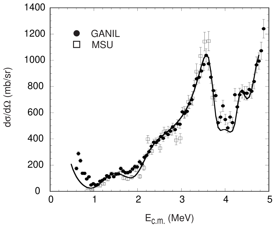
FIG. 9.: The fit of the potential model with added resonances. The full drawn curve includes the two known resonances in ¹¹Be plus a broad 3/2⁺ level around 4 MeV and a high-spin state at 5.4 MeV, which gives a good description of the full excitation function up to 4.7 MeV. Especially it should be noted that the theoretical curve now better reproduces the data at 1.6-2.0 MeV.

Of the three resonances included in the calculations, only the one at 4.33 MeV is distinctly seen in the excitation function, see Figure 9. Its position corresponds to the 3/2^- state at 2.69 MeV in ¹¹Be within 150 keV, and the cross section supports a spin of 3/2 for this resonance. The obtained width of 270 keV also agrees with the width of the 2.69 MeV level in ¹¹Be if decay by a $\ell$=1 proton is assumed. We thus conclude that the narrow resonance at 4.33 MeV in ¹¹N is the mirror of the 2.69 MeV state in ¹¹Be, both having $I^{\pi}$=3/2^-. The other resonances above 4 MeV are introduced in order to reproduce the cross section at higher energies. The experimental data is not sufficient to give conclusive determination of any parameters of these states, but the existence of resonances above 4.4 MeV is necessary to reproduce the measured cross section.

V Discussion

A The three lowest resonances in ¹¹N.

Table I presents the parameters used in different fits of the deduced excitation function in the ¹⁰C+p system. The fits were all made under the assumption of three low-lying resonances. From these data we conclude that the three lowest states in ¹¹N have I^π= 1/2⁺, 1/2^- and 5/2⁺. This is the first time all these states are identified in one single experiment. However, there have been indications of them in other reaction experiments. In the pioneering work on ¹¹N by Benenson et al. [13], where the ¹⁴N(³He,⁶He) reaction was studied, it was proposed that the resonance observed at 2.24 MeV ($\Gamma$=740 keV) was a 1/2^- state. This conclusion was based on the reaction mechanism in their experiment. Our data confirms this result and both position and width are within the experimental errors of the two experiments. The difference may probably be attributed to different approaches in extracting the resonance parameters. In a recent paper by Lepine-Szily et al. [23], a state at 2.18 MeV was observed and interpreted as a 1/2^- state, but with a width that was considerably narrower than in our work or that of Ref. [13].

The state at 1.27 MeV, which we interpret as a 1/2⁺ state, could not be seen in the two experiments in Refs. [13, 23], as the selected reactions quench the population of this state considerably. It could, however, be observed in an experiment performed at MSU where Azhari et al. [24] studied proton emission from ¹¹N produced in a ⁹Be(¹²N,¹¹N) reaction. They found indications of a double peak at low energies and by fixing the upper part of it to the parameters from Ref. [13] they arrived at an excitation energy of 1.45 MeV.

The 5/2⁺ (3.75 MeV) state was discussed in [4]. The experiment presented in [23] showed a state at 3.63 MeV with a width about 400 keV. The position of the resonance is close to ours but again the width is smaller in [23].

As well as for the 1/2⁺ and 1/2^- states, the spin value for the 5/2⁺ resonance does not leave any doubt that it is the mirror state of the 5/2⁺ level at 1.78 MeV in ¹¹Be ($\Gamma$ = 100 keV). The potential model with the parameters used for ¹¹N and given in Table I:c agrees very well for the width while the excitation energy becomes 1.63 MeV. Still we consider this as an additional support for our interpretation.

Fortune et al. [25] have predicted the splitting between $0d_{5/2}$ and $1s_{1/2}$ states in ¹¹N from the systematics of this energy difference for light nuclei, mainly assuming isobaric spin conservation. Their results can therefore be considered as a direct extrapolation of experimental data. The energy difference obtained in our work (${\Delta}E$=2.48 MeV) is close to the prediction of 2.3 MeV in [25]. The energy difference between the $1s_{1/2}$ and $0p_{1/2}$ was calculated using the complex scaling method in [26] and the value of 830 keV agrees with our data which gives 740 keV.

B Resonances above 4 MeV

We interpret the structure around 4.3 MeV as due to a sharp resonance in ¹¹N, which is the mirror state of the 2.69 MeV level in ¹¹Be, Table III. Several different experiments (see for example [22]) give the spin-parity for this ¹¹Be level as 3/2^-. The negative parity is well established from measurements of the ¹¹Li beta-decay [27, 28, 29], and by measurements of the ⁹Be(t,p)¹¹Be reaction [22]. There is also good agreement between the Cohen-Kurath prediction for the spectroscopic factor and the reduced single particle widths of these mirror states. We found very good agreement between the widths if the states undergo nucleon decay with $\ell\!=\!1$ ($j\!=\!3/2$). If the states decay with orbital momentum, $\ell\!=\!2$ ($j=3/2$), the state in ¹¹N will be at least twice as broad, and in the case of $\ell\!=\!3$ ($j\!=\!5/2$) it would be at least 3 times broader. Also, for $\ell\!=\!3$ the reduced single particle width will be too large, contradicting [30]. Using the simplified R-matrix approach, the position of the 3/2^- level was determined as 4.33 MeV. The observed cross section for the population of this state is also in accordance with a 3/2^- assignment. The calculations further indicate that about one third of the width of the 4.33 MeV state is due to the proton decay to the first excited state in ¹⁰C. Even a small branch of this decay results in a large reduced width. This indicates a large coupling of 3/2^- state to the first excited state of the core, as was recently predicted by Descouvemont [31]. In [4] we proposed a different structure for the 3/2^- state (two particles in the $1s$ state) because preliminary treatment resulted in a too small width (70 keV) for the state.

In the present experiment there is an experimental cutoff at 5.4 MeV (see Figure 3) and the excitation function increases towards this high-energy end. This is most likely due to higher-lying states but we cannot make any assignments for them based on our data. However the authors [24] had to introduce a broad ($\Gamma$= 500-1000 keV) state in the energy region around 4.6 MeV to explain the spectrum from ¹¹N decay. They proposed the broad state to be a 3/2^- state. Our data show that the 3/2^- state in ¹¹N is rather narrow, and therefore another state has to be assumed in order to explain the data in [24]. This is also a justification for the inclusion of the 3/2⁺ resonance is our R-matrix fit.

Various theoretical calculations (for recent references see [32]) have attempted to reproduce the level sequence in ¹¹Be. Most models emphasize the role of coupling between the valence neutron and the first excited 2⁺ state in ¹⁰Be in generating the parity inversion. It is well known that model assumptions influence the wave functions more than their energy eigenvalues and thus models giving the correct level sequence predict very different core excitation admixtures. For the ground state in ¹¹Be, the admixtures given by theoretical calculations vary from 7% [31, 33] to 75% [34]. Theoretical results are frequently compared to spectroscopic factors obtained from nucleon transfer reactions. The single-particle spectroscopic factors for ¹¹Be have been obtained from ¹⁰Be(d,p) reactions [30]. Even if the theory of stripping reactions is very well developed, many parameters are involved in the extraction of these results from the data. Evaluating single-particle nucleon widths using a potential model involves fewer parameters. For the lowest states of ¹¹N we obtained the reduced widths given in Table II. For the s_1/2 state we have a reduced width of $\approx$1 which, taking the 15% experimental error in the width into account, indicates that no large core-excitation admixtures are needed to describe the ground states of ¹¹N and ¹¹Be.

VI Summary

The excitation function in the ¹⁰C+p system has been studied using elastic resonance scattering. The low-energy part was analyzed in a potential model while the high-energy part was described in a simplified R-matrix approach. The ground state and the first two excited states in the unbound nucleus ¹¹N was found to have the spin-parity sequence of 1/2⁺, 1/2^- and 5/2⁺ which is identical to that found in its mirror partner ¹¹Be. A narrow 3/2^- state at 4.33 MeV was identified as the mirror state of the 2.69 MeV state in ¹¹Be. The energies and widths of the observed states are listed in Table IV. The agreement among experiments as well as between our results and theoretical calculations

[

TABLE IV.: A summary of all experimental and theoretical results on ¹¹N. $E_{r}$ and $\Gamma_{r}$ denote the resonance energy and the width of the resonance, respectively. The error bars in this work include the systematic errors (25 keV in the c.m. frame) as well as the spread in results obtained for different potential parameters that all fit the data.

	1/2+		1/2-		5/2+
Ref.	$E_{r}$	$\Gamma_{r}$	$E_{r}$	$\Gamma_{r}$	$E_{r}$	$\Gamma_{r}$
Experimental papers
This work	$1.27^{+0.18}_{-0.05}$	$1.44\pm 0.2$	$2.01^{+0.15}_{-0.05}$	$0.84\pm 0.2$	$3.75\pm 0.05$	$0.60\pm 0.05$
[13]	-	-	$2.24\pm 0.1$	$0.74\pm 0.1$	-	-
[23]	-	-	$2.18\pm 0.05$	$0.44\pm 0.08$	$3.63\pm 0.05$	$0.40\pm 0.08$
[24]a	$1.45\pm 0.40$	$>0.4$	$2.24\pm 0.1$	$0.74\pm 0.1$	-	-
Theoretical papers
[35]a	1.54	0.62	$2.24\pm 0.1$	$0.74\pm 0.1$	3.74	0.3
[25]	$1.60\pm 0.22$	$2.1^{+1.0}_{-0.7}$	2.49	1.45	3.90	0.88
[36]b	1.4	1.31	2.21	0.91	3.88	0.72
[31]	1.1	0.9	1.6	0.3	3.8	0.6
[37]	1.2	1.2	2.1	1.0	3.7	1.0
aFor the $1/2^{-}$ state the results from [13].
bThe results obtained with $r_{0}=1.45$ fm is presented.

] are very satisfactory.

The quasi-stationary character of ¹¹N states was used to evaluate the reduced single-particle widths for the identified states. This result indicates small coupling between the valence nucleon in the ground state ¹¹N and the first excited 2⁺ state in ¹⁰C, and the same conclusion should be valid for ¹¹Be.

The experimental technique to use elastic-resonance scattering with radioactive beams has proven to be a very efficient tool for investigations beyond the dripline.

VII Acknowledgments

The authors thank Prof. M. Zhukov and Prof. F. Barker for valuable discussions. The work was partially supported by the National Science Foundation under grant PHY95-28844. The work was also partly supported by a grant from RFBR. S. B. acknowledges the support of the REU program under grant PHY94-24140.

REFERENCES

- [1] K. P. Artemov et al., Sov. J. Nucl. Phys. 52, 634 (1990).
- [2] V. Z. Gol’dberg et al., Phys. At. Nucl. 60, 1061 (1997).
- [3] V. Z. Goldberg and A. E. Pakhomov, Phys. At. Nucl. 56, 1167 (1993).
- [4] L. Axelsson et al., Phys. Rev. C 54, R1511 (1996).
- [5] R. Coszach et al., Phys. Rev. C 50, 1695 (1994).
- [6] M. Benjelloun et al., Nucl. Instr. and Meth. in Phys. Res. A 321, 521 (1992).
- [7] B. Jonson and K. Riisager, Phil. Trans. R. Soc. Lond. A. 356, 2063 (1998).
- [8] R. Anne et al., Phys. Lett. B 304, 55 (1993).
- [9] F. M. Nunes, I. J. Thompson, and R. C. Johnson, Nucl. Phys. A 596, 171 (1996).
- [10] D. J. Millener, J. W. Olness, E. K. Warburton, and S. S. Hanna, Phys. Rev. C 28, 497 (1983).
- [11] I. Talmi and I. Unna, Phys. Rev. Lett. 4, 469 (1960).
- [12] H. Sagawa, B. A. Brown, and H. Esbensen, Phys. Lett. B 309, 1 (1993).
- [13] W. Benenson et al., Phys. Rev. C 9, 2130 (1974).
- [14] G. Breit and E. Wigner, Phys. Rep. 49, 519 (1936).
- [15] P. E. Hodgson, E. Gadioli, and E. Gadioli Erba, Introductory nuclear physics (Oxford science publications, Oxford, 1997).
- [16] R. A. Laubenstein and M. J. W. Laubenstein, Phys. Rev. 84, 18 (1951).
- [17] J. B. Marion and F. C. Young, Nuclear reaction analysis (graphs and tables) (North-Holland Publishing company, Amsterdam, 1968).
- [18] D. L. Auton, Nucl. Phys. A 157, 305 (1970).
- [19] H. L. Jackson and A. I. Galonsky, Phys. Rep. 89, 370 (1953).
- [20] F. Ajzenberg-Selove, Nucl. Phys. A 506, 1 (1990).
- [21] K. S. Krane, Introductory Nuclear Physics (John Wiley and Sons, New York, 1988).
- [22] G.-B. Liu and H. T. Fortune, Phys. Rev. C 42, 167 (1990).
- [23] A. Lépine-Szily et al., Phys. Rev. Lett. 80, 1601 (1998).
- [24] A. Azhari et al., Phys. Rev. C 57, 628 (1998).
- [25] H. T. Fortune, D. Koltenuk, and C. K. Lau, Phys. Rev. C 51, 3023 (1995).
- [26] A. Aoyama, N. Itagaki, K. Kato, and K. Ikeda, Phys. Rev. C 57, 975 (1998).
- [27] N. Aoi et al., Nucl. Phys. A 616, 181c (1997).
- [28] D. J. Morrisey et al., Nucl. Phys. A 627, 222 (1997).
- [29] I. Mukha et al., To be published.
- [30] B. Zwieglinski, W. Benenson, and R. H. G. Robertson, Nucl. Phys. A 315, 124 (1979).
- [31] P. Descouvemont, Nucl. Phys. A 615, 261 (1997).
- [32] S. Fortier et al., Phys. Lett. B 461, 22 (1999).
- [33] N. Vinh Mau, Nucl. Phys. A 592, 33 (1995).
- [34] I. Ragnarsson, in Proc. of the Int. Workshop on The Science of Intense Radioactive Beams, LA-11964-c (, Los Alamos, 1990), p. 199.
- [35] R. Sherr, Coulomb shifts in A=11 quartet (IMME), Private communication, 1995.
- [36] F. C. Barker, Phys. Rev. C 53, 1449 (1996).
- [37] S. Grévy, O. Sorlin, and N. Vinh Mau, Phys. Rev. C 56, 2885 (1997).