Toward a phenomenological approach to the clustering of heavy particles in turbulent flows

Abstract

A simple model accounting for the ejection of heavy particles from the vortical structures of a turbulent flow is introduced. This model involves a space and time discretization of the dynamics and depends on only two parameters: the fraction of space-time occupied by rotating structures of the carrier flow and the rate at which particles are ejected from them. The latter can be heuristically related to the response time of the particles and hence measure their inertia. It is shown that such a model reproduces qualitatively most aspects of the spatial distribution of heavy particles transported by realistic flows. In particular the probability density function of the mass $m$ in a cell displays an power-law behavior at small values and decreases faster than exponentially at large values. The dependence of the exponent of the first tail upon the parameters of the dynamics is explicitly derived for the model. The right tail is shown to decrease as $\exp(-Cm\log m)$. Finally, the distribution of mass averaged over several cells is shown to obey rescaling properties as a function of the coarse-grain size and of the ejection rate of the particles. Contrarily to what has been observed in direct numerical simulations of turbulent flows (Bec et al., nlin.CD/0608045), such rescaling properties are only due in the model to the mass dynamics of the particles and do not involve any scaling properties in the spatial structure of the carrier flow.

1 Introduction

Understanding the dynamics of small-size tracer particles or of a passive field transported by an incompressible turbulent flow plays an important role in the description of several natural and industrial phenomena. For instance it is well known that turbulence has the property to induce an efficient mixing over the whole range of length and time scales spanned by the turbulent cascade of kinetic energy (see e.g. [1]). Describing quantitatively such a mixing has consequences in the design of engines, in the prediction of pollutant dispersion or in the development of climate models accounting for transport of salinity and temperature by large-scale ocean streams.

However, in some settings, the suspended particles have a finite size and a mass density very different from that of the fluid. Thus they can hardly be modeled by tracers because they have inertia. In order to fully describe the dynamics of such inertial particles, one has to consider many forces that are exerted by the fluid even in the simple approximation where the particle is a hard sphere much smaller than the smallest active scale of the fluid flow [2]. Nevertheless the dynamics drastically simplifies in the asymptotics of particles much heavier than the carrier fluid. In that case, and when buoyancy is neglected, they interact with the flow only through a viscous drag, so that their trajectories are solutions to the Newton equation :

$$\frac{d^{2}\bm{X}}{dt^{2}}=-\frac{1}{\tau}\left[\frac{d\bm{X}}{dt}-\bm{u}(\bm{X},t)\right]\,,$$ (1)

where $\bm{u}$ denotes the underlying fluid velocity field and $\tau$ is the response time of the particles. Even if the carrier fluid is incompressible, the dynamics of such heavy particles lags behind that of the fluid and is not volume-preserving. At large times particles concentrate on singular sets evolving with the fluid motion, leading to the appearance of strong spatial inhomogeneities dubbed preferential concentrations. At the experimental level such inhomogeneities have been known for a long time (see [3] for a review). At present the statistical description of particle concentration is a largely open question with many applications. We mention the formation of rain droplets in warm clouds [4], the coexistence of plankton species [5], the dispersion in the atmosphere of spores, dust, pollen, and chemicals [6], and the formation of planets by accretion of dust in gaseous circumstellar disks [7].

The dynamics of inertial particles in turbulent flows involves a competition between two effects: on the one hand particles have a dissipative dynamics, leading to the convergence of their trajectories onto a dynamical attractor [8], and on the other hand, the particles are ejected from the coherent vortical structures of the flow by centrifugal inertial forces [9]. The simultaneous presence of these two mechanisms has so far led to the failure of all attempts made to obtain analytically the dynamical properties or the mass distribution of inertial particles. In order to circumvent such difficulties a simple idea is to tackle independently the two aspects by studying toy models, either for the fluid velocity field, or for the particle dynamics that are hopefully relevant in some asymptotics (small or large response times, large observation scales, etc.). Recently an important effort has been made in the understanding of the dynamics of particles suspended in flows that are $\delta$-correlated in time, as in the case of the well-known Kraichnan model for passive tracers [10]. Such settings, which describe well the limit of large response time of the particles, allows one to obtain closed equations for density correlations by Markov techniques. The $\delta$-correlation in time, of course, rules out the presence of any persistent structure in the flow; hence any observed concentrations can only stem from the dissipative dynamics. Most studies in such simplified flows dealt with the study of the separation between two particles [11, 12, 13, 14, 15].

Recent numerical studies in fully developped turbulent flows [16] showed that the spatial distribution of particles at lengthscales within the inertial range are strongly influenced by the presence of voids at all active scales spanned by the turbulent cascade of kinetic energy. The presence of these voids has a noticeable statistical signature on the probability density function (PDF) of the coarse-grained mass of particles which displays an algebraic tail at small values. To understand at least from a qualitative and phenomenological viewpoint such phenomena, it is clearly important to consider flows with persistent vortical structures which are ejecting heavy particles. For this purpose, we introduce in this paper a toy model where the vorticity field of the carrier flow is assumed piecewise constant in both time and space and takes either a finite fixed value $\omega$ or vanishes. In addition to this crude simplification of the spatial structure of the fluid velocity field we assume that the particle mass dynamics obeys the following rule: during each time step there is a mass transfer between the cells having vorticity $\omega$ toward the neighboring cells where the vorticity vanishes. The amount of mass escaping to neighbors is at most a fixed fraction $\gamma$ of the mass initially contained in the ejecting cell. We show that such a simplified dynamics reproduces many aspects of the mass distribution of heavy particles in incompressible flow. In particular, we show that the PDF of the mass of inertial particles has an algebraic tail at small values and decreases as $\exp(-A\,m\,\log m)$ when $m$ is large. Analytical predictions are confirmed by numerical experiments in one and two dimensions.

In section 2 we give some heuristic motivations for considering such a model and a qualitative relation between the ejection rate $\gamma$ and the response time $\tau$ of the heavy particles. Section 3 consists in a precise definition of the model in one dimension and in its extension to higher dimensions. Section 4 is devoted to the study in the statistical steady state of the PDF of the mass in a single cell. In section 5 we study the mass distribution averaged over several cells to gain some insight on the scaling properties in the mass distribution induced by the model. Section 6 encompasses concluding remarks and discussions on the extensions and improvements of the model that are required to get a more quantitative insight on the preferential concentration of heavy particles in turbulent flows.

2 Ejection of heavy particles from eddies

The goal of this section is to give some phenomenological arguments explaining why the model which is shortly described above, might be of relevance to the dynamics of heavy particles suspended in incompressible flows. In particular we explain why a fraction of the mass of particles exits a rotating region and give a qualitative relation between the ejection rate $\gamma$ and the response time $\tau$ entering the dynamics of heavy particles. For this we focus on the two-dimensional case and consider a cell of size $\ell$ where the fluid vorticity $\omega$ is constant and the fluid velocity vanishes at the center of the cell. This amounts to considering that the fluid velocity is linear in the cell with a profile given to leading order by the strain matrix. Having a constant vorticity in a two-dimensional incompressible flow means that we focus on cases where the two eigenvalues of the strain matrix are purely imaginary complex conjugate. The particle dynamics reduces to the second-order two-dimensional linear system

$$\frac{d^{2}\bm{X}}{dt^{2}}=-\frac{1}{\tau}\,\frac{d\bm{X}}{dt}+\frac{\omega}{\tau}\left[\!\!\!\begin{array}[]{rl}0&1\\ -1&0\end{array}\right]\,\bm{X}\,.$$ (2)

It is easily checked that the four eigenvalues of the evolution matrix are the following complex conjugate

$$\lambda_{\pm,\pm}=\frac{-1\pm\sqrt{1\pm 4i\tau\omega}}{2\tau}\,.$$ (3)

Only $\lambda_{+,-}$ and $\lambda_{+,+}$ have a positive real part which is equal to

$$\mu=\frac{-1+\frac{1}{2}\sqrt{2\sqrt{1+16\tau^{2}\omega^{2}}+2}}{2\tau}\,.$$ (4)

This means that the distance of the particles to the center of the cell increases exponentially fast in time with a rate $\mu$. If we now consider that the particles are initially uniformly distributed inside the cell, we obtain that the mass of particles remaining in it decreases exponentially fast in time with a rate equal to $-2\mu$. Namely the mass of particles which are still in the cell at time $T$ is

$$m(T)=m(0)\,(1-\gamma)=m(0)\,\exp\!\!\left[-\frac{T}{\tau}\!\left(-1+\frac{1}{2}\sqrt{2\sqrt{1+16\tau^{2}\omega^{2}}+2}\right)\!\right]\!\!.$$ (5)

The rate $\gamma$ at which particles are expelled from the cell depends upon the response time $\tau$ of the particles and upon two characteristic times associated to the fluid velocity. The first is the time length $T$ of the ejection process which is given by the typical life time of the structure with vorticity $\omega$. The second time scale is the turnover $\omega^{-1}$ which measures the strength of the eddy. There are hence two dimensionless parameters entering the ejection rate $\gamma$: the Stokes number ${\mbox{\it St}}=\tau\omega$ giving a measure of inertia and the Kubo number ${\mbox{\it Ku}}=T\omega$ which is the ratio between the correlation time of structures and their eddy turnover time. One hence obtain the following estimate of the ejection rate

$$\gamma=1-\exp\!\!\left[-\frac{{\mbox{\it Ku}}}{{\mbox{\it St}}}\,\left(-1+\frac{1}{2}\sqrt{2\sqrt{1+16{\mbox{\it St}}^{2}}+2}\right)\!\right]\!\!.$$ (6)

The graph of the fraction of particles ejected from the cell as a function of the Stokes number is represented in figure 1 for three different values of the Kubo number. The function goes to zero as Ku St in the limit ${\mbox{\it St}}\to 0$ and as ${\mbox{\it Ku}}\,{\mbox{\it St}}^{-1/2}$ in the limit ${\mbox{\it St}}\to\infty$. It reaches a maximum which is an indication of a maximal segregation of the particles, for ${\mbox{\it St}}\approx 1.03$ independently of the value of Ku.

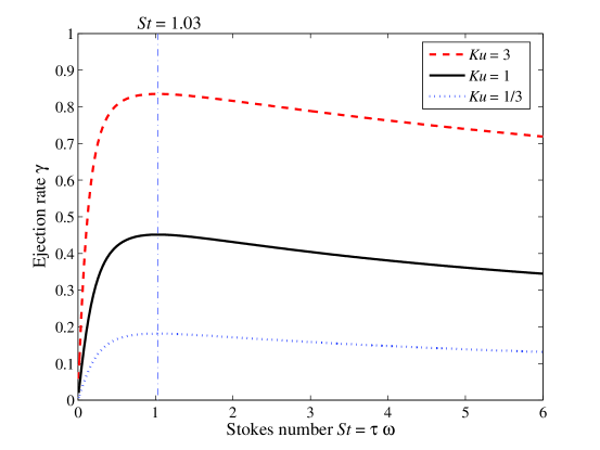
Figure 1: Fraction of the mass of particles that are uniformly distributed and ejected from an eddy of arbitrary size $\ell$ as a function of the Stokes number ${\mbox{\it St}}=\tau\omega$. The various curves refer to different values of the Kubo number Ku as labeled.

In three dimensions, one can extend the previous approach to obtain an ejection rate for cells with a uniform rotation, i.e. a constant vorticity $\bm{\omega}$. There are however two main difficulties. The first is that in three dimensions the eigenvalues of the strain matrix in rotating regions are not anymore purely imaginary but have a real part given by the opposite of the rate in the stretching direction. Such a vortex stretching has to be considered to match observation in real flows. The second difficulty stems from the fact that the vorticity is now a vector and has a direction, so that ejection from the cell can be done only in the directions perpendicular to the direction of $\bm{\omega}$. These two difficulties imply that the spectrum of possible ejection rates is much broader than in the two-dimensional case. However the rough qualitative picture is not changed.

3 A simple mass transport model

We here describe with details the model in one dimension and mention at the end of the section how to generalize it to two and higher dimensions. Let us consider a discrete partition of an interval in $N$ small cells. Each of these cell is associated to a mass which is a continuous variable. We denote by $m_{j}(n)$ the mass in the $j$-th cell at time $t=n$. At each integer time we choose randomly $N$ independent variables; $\Omega_{j}=1$ with probability $p$ and $\Omega_{j}=0$ with probability $1-p$. The evolution of mass between times $n$ and $n+1$ is given by:

$$m_{j}(n+1)=\left\{\begin{array}[]{ll}m_{j}(n)-\frac{\gamma}{2}\,\left[2-\Omega_{j-1}-\Omega_{j+1}\right]\,m_{j}(n)&\mbox{if }\Omega_{j}=1\,,\\ m_{j}(n)+\frac{\gamma}{2}\,\left[\Omega_{j-1}\,m_{j-1}(n)+\Omega_{j+1}\,m_{j+1}(n)\right]&\mbox{if }\Omega_{j}=0\,.\end{array}\right.$$ (7)

In other terms, when $\Omega_{j}=1$, the $j$-th cell looses mass if $\Omega_{j-1}=0$ or $\Omega_{j+1}=0$, and when $\Omega_{j}=0$, it gains mass if $\Omega_{j-1}=1$ or $\Omega_{j+1}=1$. The flux of mass between the $j$-th and the $(j+1)$-th cell is proportional $\Omega_{j}-\Omega_{j+1}$ (see figure 2).

Figure 2: Sketch of the dynamics in the one-dimensional case: the fluxes of mass are represented as arrows. A cross means no flux.

In particular, if $\Omega_{j}=\Omega_{j+1}$, no mass is transfered between cells. When the system is supplemented by periodic boundary conditions between the cells $N$ and 1, it is clear that the total mass is conserved. Hereafter we assume that the mass is initially $m_{j}=1$ in all cells., so that the total mass is $\sum_{j}m_{j}=N$. Spatial homogeneity of the random process $\Omega_{j}$ implies that $\langle m_{j}\rangle=1$ for all later times, where the angular brackets denote average with respect to the realizations of the $\Omega_{j}$’s.

A noticeable advantage of such a model for mass transportation is that the mass field $\bm{m}=(m_{1},\dots,m_{N})$ defines a Markov process. Its probability distribution $p_{N}(\bm{m},n+1)$ at time $n+1$, which is the joint PDF of the masses in all cells, is related to that at time $n$ by a Markov equation, which under its general form can be written as

$$p_{N}(\bm{m},n+1) = \int d^{N}\!m^{\prime}\,p_{N}(\bm{m}^{\prime},n)\,P[\bm{m}^{\prime}\to\bm{m}]$$ (8)

$$= \int d^{N}\!m^{\prime}\,p_{N}(\bm{m}^{\prime},n)\int d^{N}\!\Omega\,\,p(\bm{\Omega})\,P[\bm{m}^{\prime}\to\bm{m}|\bm{\Omega}],$$

where $P[\bm{m}^{\prime}\to\bm{m}|\bm{\Omega}]$ denotes the transition probability from the field $\bm{m}^{\prime}$ to the field $\bm{m}$ conditioned on the realization of $\bm{\Omega}=(\Omega_{1},\dots,\Omega_{N})$. In our case it takes the form

$$P[\bm{m}^{\prime}\to\bm{m}|\bm{\Omega}]=\prod_{j=1}^{N}\delta[m_{j}-(m_{j}^{\prime}+\mu_{j-1}(n)-\mu_{j}(n))]\,.$$ (9)

The variable $\mu_{j}$ denotes here the flux of mass between the $j$-th and the $(j+1)$-th cell. It is a function of $\Omega_{j}$, $\Omega_{j+1}$, and of the mass contained in the two cells. It can be written as

$$\mu_{j}(n)=\frac{\gamma}{2}\!\left[\Omega_{j}(n)(1-\Omega_{j+1}(n))m^{\prime}_{j}(n)-\Omega_{j+1}(n)(1-\Omega_{j}(n))m^{\prime}_{j+1}(n)\right]\!.$$ (10)

In the particular case we are considering, the joint probability of the $\Omega_{j}$’s factorizes and we have

$$p(\Omega_{j})=p\,\delta(\Omega_{j}-1)+(1-p)\,\delta(\Omega_{j})\,,$$ (11)

so that the Markov equation (8) can be written in a rather explicit and simple manner.

The extension of the model to two dimensions is straightforward. The mass transfer out from a rotating cell can occur to one, two, three or four of its direct nearest neighbors (see figure 3 left). One can similarly derive a Markov equation which is similar to (8) for the joint PDF $p_{N,N}(\mathbb{M},n)$ at time $n$ of the mass configuration $\mathbb{M}=\{m_{i,j}\}_{1\leq i,j\leq N}$. The transition probability reads in that case

$$P[\mathbb{M}^{\prime}\to\mathbb{M}|\bm{\Omega}]=\prod_{i=1}^{N}\prod_{j=1}^{N}\delta[m_{i,j}-(m_{i,j}^{\prime}+\mu^{(1)}_{i-1,j}-\mu^{(1)}_{i,j})+\mu^{(2)}_{i,j-1}-\mu^{(2)}_{i,j})]\,.$$ (12)

where the fluxes now take the form

$$\mu^{(1)}_{i,j}=\frac{\gamma}{4}\left[\Omega_{i,j}(1-\Omega_{i+1,j})\,m^{\prime}_{i,j}-\Omega_{i+1,j}(1-\Omega_{i,j})\,m^{\prime}_{i+1,j}\right]$$ (13)

and $\mu^{(2)}_{i,j}$ defined by inverting $i$ and $j$ in the definition of $\mu^{(1)}_{i,j}$.

After a large number of time steps, a statistically steady state is reached. The stationary distribution is obtained assuming that $p_{N,N}(\mathbb{M},n)=p_{N,N}(\mathbb{M})$ is independent of $n$ in the Markov equation (8). In this stationary state the mass fluctuates around its mean value $1$ corresponding to a uniform distribution; strong deviations at small masses can be qualitatively observed (see figure 3 right).

     

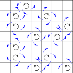
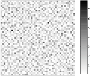
Figure 3: Left: sketch of the ejection model in two dimensions; the rotating cells are designated by small eddies; the flux of mass (blue arrows) is from the rotating cells to those without any eddy. Right: snapshot of the distribution of mass in the statistically steady regime for a domain of $50^{2}$ cells with $p=0.75$; white squares are almost empty cells and the darker regions correspond to cells where the mass is concentrated.

The model can be easily generalized to arbitrary space dimension. However, as we have seen in previous section, besides its interest from a purely theoretical point of view, the straightforward extension to the three-dimensional case might not be relevant to describe concentrations of inertial particles in turbulent flows.

4 Distribution of mass

Let us consider first the one-dimensional case in the statistically stationary regime. After integrating (8), one can express the single-point mass PDF $p_{1}$ in terms of the three-point mass distribution $p_{3}$ at time $n$

$$p_{1}(m_{j}) = \int\!\!dm^{\prime}_{j-1}\,dm^{\prime}_{j}\,dm^{\prime}_{j+1}\,p_{3}(m^{\prime}_{j-1},m^{\prime}_{j},m^{\prime}_{j+1})\int\!\!d\Omega_{j-1}\,d\Omega_{j}\,d\Omega_{j+1}\times$$ (14)

$$\quad p(\Omega_{j-1})\,p(\Omega_{j})\,p(\Omega_{j+1})\,\delta[m_{j}-(m^{\prime}_{j}+\mu_{j-1}-\mu_{j})]\,.$$

We then explicit all possible fluxes, together with their probabilities, by considering all possible configurations of the spin vorticity triplet $(\Omega_{j-1},\Omega_{j},\Omega_{j+1})$. The results are summarized in table 1. This leads to rewrite the one-point PDF as

$$p_{1}(m) = \left[p^{3}+(1-p)^{3}\right]\,p_{1}(m)+\frac{2p^{2}\,(1-p)}{1-\gamma/2}\,p_{1}\!\left(\frac{m}{1-\gamma/2}\right)+$$ (15)

$$+ \frac{p\,(1-p)^{2}}{1-\gamma}\,p_{1}\!\left(\frac{m}{1-\gamma}\right)+2p\,(1-p)^{2}\!\int_{0}^{2m/\gamma}\!\!\!\!\!\!\!\!\!\!dm^{\prime}\,p_{2}\!\left(m^{\prime},m-\frac{\gamma}{2}m^{\prime}\right)+$$

$$+ p^{2}(1-p)\!\int_{0}^{2m/\gamma}\!\!\!\!\!\!\!\!\!\!dm^{\prime}\!\!\!\int_{0}^{2m/\gamma-m^{\prime}}\!\!\!\!\!\!\!\!\!\!\!\!\!\!\!\!\!\!dm^{\prime\prime}\,p_{3}\!\left(m^{\prime},m-\frac{\gamma}{2}(m^{\prime}+m^{\prime\prime}),m^{\prime\prime}\right).$$

The first term on the right-hand side comes from realizations with no flux. The second term is ejection to one neighbor and the third to two neighboring cells. The fourth term involving an average over the two-cell distribution is related to events when mass is transfered from a single neighbor to the considered cell. Finally, the last term accounts for transfers from the two direct neighbors. Note that, in order to write (15), we made use of the fact that $p_{2}(x,y)=p_{2}(y,x)$.

Table 1: Enumeration of all possible configurations of the spin vorticity $\Omega$ in three neighboring cells, together with their probabilities and the associated mass fluxes.

• $\Omega_{j-1}$	$\Omega_{j}$	$\Omega_{j+1}$	Prob	$\mu_{j-1}$	$\mu_{j}$
  0	0	0	$(1-p)^{3}$	0	0
  0	0	1	$p\,(1-p)^{2}$	0	$-\gamma m^{\prime}_{j+1}/2$
  0	1	0	$p\,(1-p)^{2}$	$-\gamma m^{\prime}_{j}/2$	$\gamma m^{\prime}_{j}/2$
  0	1	1	$p^{2}\,(1-p)$	$-\gamma m^{\prime}_{j}/2$	0
  1	0	0	$p\,(1-p)^{2}$	$\gamma m^{\prime}_{j-1}/2$	0
  1	0	1	$p^{2}\,(1-p)$	$\gamma m^{\prime}_{j-1}/2$	$-\gamma m^{\prime}_{j+1}/2$
  1	1	0	$p^{2}\,(1-p)$	0	$\gamma m^{\prime}_{j}/2$
  1	1	1	$p^{3}$	0	0

Numerical simulations of this one-dimensional mass transport model are useful to grab qualitative information on $p_{1}$. Figure 4 represents the functional form of $p_{1}$ in the stationary regime for various values of the ejection rate $\gamma$ and for $p=1/2$. The curves are surprisingly similar to measurements of the spatial distribution of heavy particles suspended in homogeneous isotropic turbulent flows [3, 16]. This gives strong evidence that, on a qualitative level, the model we consider reproduces rather well the main mechanisms of preferential concentration. More specifically, a first observation is that in both settings the probability density functions display an algebraic behavior for small masses. This implies that the ejection from cells with vorticity one has a strong statistical signature. A second observation is that at large masses, the PDF decays faster than exponentially, as also observed in realistic flows. As we will now see these two tails can be understood analytically for the model under consideration.

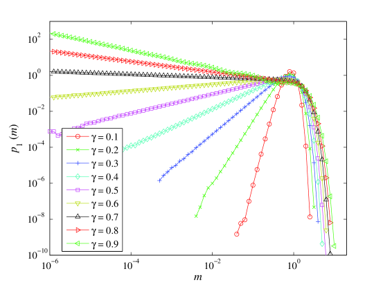
Figure 4: Log-log plot of the one-point PDF of the mass in one dimension for $p=1/2$ and different values of the parameter $\gamma$ as labeled. The integration was done on a domain of $2^{16}=65536$ cells and time average wee performed during $10^{6}$ time steps after a statistical steady state is reached.

We here first present an argument explaining why an algebraic tail is present at small masses. For this we exhibit a lower bound of the probability $P^{<}(m)$ that the mass in the given cell is less than $m$. Namely, we have

$$P^{<}(m)={\rm Prob}(m_{j}(n)<m)\geq{\rm Prob}\,(\mathcal{A})\,,$$ (16)

where $\mathcal{A}$ is a set of space-time realizations of $\Omega$ such that the mass in the $j$-th cell at time $n$ is smaller than $m$. For instance we can choose the set of realizations which are ejecting mass in the most efficient way: during a time $N$ before $n$, the $j$-th cell has spin vorticity 1 and its two neighbors have 0. The mass at time $n$ is related to the mass at time $n-N$ by

$$m_{j}(n)=(1-\gamma)^{N}m_{j}(n-N)\,,\ \mbox{ that is }\ N=\frac{\log[m_{j}(n-N)/m_{j}(n)]}{\log(1-\gamma)}\,.$$ (17)

The probability of such a realization is clearly $p^{N}\,(1-p)^{2N}$. Replacing $N$ by the expression obtained in (17), we see that

$${\rm Prob}\,(\mathcal{A})=\left[\frac{m_{j}(n)}{m_{j}(n-N)}\right]^{\beta}\mbox{ with }\beta=\frac{\log[p(1-p)^{2}]}{\log(1-\gamma)}.$$ (18)

After averaging with respect to the initial mass $m_{j}(n-N)$, one finally obtains

$$P^{<}(m)\geq A\,m^{\beta}.$$ (19)

Hence the cumulative probability of mass cannot have a tail faster than a power law at small arguments. It is thus reasonable to make the ansatz that $p_{1}(m)$ have an algebraic tail at $m\to 0$, i.e. that $p_{1}(m)\simeq Cm^{\alpha}$. To obtain how the exponent $\alpha$ behaves as a function of the parameters $\gamma$ and $p$, this ansatz is injected in the stationary version of the Markov equation (15). One expects that the small-mass behavior involves only the terms due to ejection from a cell, namely the three first terms in the r.h.s. of (15), and that the terms involving averages of the two-point and three-point PDFs give only sub-dominant contributions. This leads to

$$Cm^{\alpha} \approx C\left[p^{3}+(1-p)^{3}\right]m^{\alpha}+C\,\frac{2p^{2}(1-p)}{1-\gamma/2}\left[\frac{m}{1-\gamma/2}\right]^{\alpha}+$$ (20)

$$+C\,\frac{p(1-p)^{2}}{1-\gamma}\left[\frac{m}{1-\gamma}\right]^{\alpha}\,.$$

Equating the various constants we finally obtain that the exponent $\alpha$ satisfies

$$\frac{2p}{(1-\gamma/2)^{\alpha+1}}+\frac{(1-p)}{(1-\gamma)^{\alpha+1}}=3\,.$$ (21)

Note that the actual exponent $\alpha$ given by this relation is different from the lower-bound $\beta+1$ obtained above in (18) and (19). However it is easily checked that $\alpha$ approach the lower bound when $p\to 0$. As seen from figure 5, formula (21) is in good agreement with numerics.

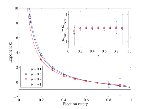
Figure 5: Scaling exponent $\alpha$ as a function of the ejection rate $\gamma$ for three different values of $p$ as labeled. The solid lines represents the prediction given by (21); the error bars are estimated from the maximal deviation of the logarithmic derivative from the estimated value. Inset: difference between the numerical estimation and the value predicted by theory.

Note that the large error bars obtained for $p$ small and $\gamma$ large are due to the presence of logarithmic oscillations in the left tail of the PDF of mass. This log periodicity is slightly visible for $\gamma=0.9$ in figure 4. It occurs when the spreading of the distribution close to the mean value $m=1$ is much smaller than the rate at which mass is ejected. This results in the presence of bumps in the PDF at values of $m$ which are powers of $1-2\gamma$. Notice that for all values of $p$, one has $\alpha\leq 0$ when $\gamma\geq 2/3$. However, according to the estimate (6), values of the ejection rate larger than $2/3$ can be attained only for large enough Kubo numbers. This is consistent with the fact that power-law tails with a negative exponent were not observed in the direct numerical simulations of turbulent fluid flows [16] where ${\mbox{\it Ku}}\approx 1$.

It is much less easy to get from numerics the behavior of the right tail of the mass PDF $p_{1}(m)$. As seen from figure 4, there was no events recorded where the mass is larger than roughly ten times its average. We however present now an argument suggesting that the tail is faster than exponential, and more particularly that $\log p_{1}(m)\propto-m\,\log m$ when $m\gg 1$. We first observe that in order to have a large mass in a given cell, one needs to transfer to it the mass coming form a large number $M$ of neighboring cells. Estimating the probability of having a large mass is equivalent to understand the probability of such a transfer. For moving mass from the $j$-th cell to the $(j-1)$-th cell, the best configuration is clearly $(\Omega_{j-1},\Omega_{j},\Omega_{j+1})=(0,1,1)$. After $N$ time steps with this configuration, the fraction of mass transfered is $1-(1-\gamma/2)^{N}$. This process is then repeated for moving mass to the second neighbor, and so on. After order $M$ iterations, the mass in the $M$-th neighbor is

$$m=\frac{1-\left[1-(1-\gamma/2)^{N}\right]^{M}}{(1-\gamma/2)^{N}}\,.$$ (22)

This means that

$$M=M(m,N)=\frac{\log\left[1-m(1-\gamma/2)^{N}\right]}{\log\left[1-(1-\gamma/2)^{N}\right]}\,,$$ (23)

with the condition that $N>-(\log m)/[\log(1-\gamma/2)]$. The probability of this whole process of mass transfer is

$$\mathcal{P}=\left[p^{2}(1-p)\right]^{N\,M}=\exp\left[\log(p^{2}(1-p))\,N\,M(m,N)\right]\,.$$ (24)

All the processes of this type will contribute terms in the right tail of the mass PDF. The dominant behavior is given by choosing $N=N^{\star}$ such that $N^{\star}\,M(m,N^{\star})$ is minimal. Such a minimum cannot be written explicitly. One however notices that, on the one hand, if $N$ is much larger than its lower bound (i.e. $N\gg-(\log m)/[\log(1-\gamma/2)]$), then $N\,M(m,N)\gg-m(\log m)/[\log(1-\gamma/2)]$. On the other hand when $N$ is chosen of the order of $\log m$, then $N\,M(m,N)\propto m\,\log m$. This suggests that the minimum is attained for $N^{\star}\propto\log m$. Finally, such estimates lead to predict that the right tail of the mass probability density function behaves as

$$p_{1}(m)\propto\exp\left[-C\,m\,\log m\right]\,,$$ (25)

where $C$ is a positive constant that depends upon the parameters $p$ and $\gamma$. As seen in figure 6, such a behavior is confirmed by numerical experiments.

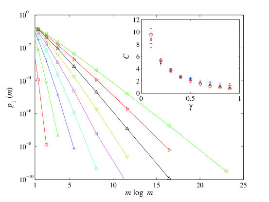
Figure 6: Lin-log plot of the one-point PDF of the mass $m$ in one dimension represented as a function of $m\log m$ for $p=1/2$ and various values of the parameter $\gamma$ as labeled; the different colors and symbols are the same as those used in figure 4. Inset: behavior of the constant $C$ appearing in (25) as a function of the ejection rate $\gamma$ for three different values of the fraction of space $p$ occupied by eddies (blue crosses: $p=0.1$, black times: $p=0.5$, red circles: $p=0.9$).

The estimations of the left and right tails of the distribution of mass in a given cell can be extended to the two-dimensional case. The results do not qualitatively change. The exponent $\alpha$ of the algebraic behavior at small masses is given as a solution of

$$\frac{4p^{3}}{(1-\gamma/4)^{\alpha+1}} + \frac{6p^{2}(1-p)}{(1-\gamma/2)^{\alpha+1}}+\frac{4p(1-p)^{2}}{(1-3\gamma/4)^{\alpha+1}}+$$ (26)

$$+ \frac{(1-p)^{3}}{(1-\gamma)^{\alpha+1}}=5(1-p+p^{2})\,.$$

By arguments which are similar to the one-dimensional case and which are not detailed here, one obtains also that $\log p_{1}(m)\propto-m\,\log m$. Numerical experiments in two dimensions confirm these behaviors of the mass probability distribution. As seen from figure 7 an algebraic behavior of the left tail of the PDF of $m$ is observed and the value of the exponent is in good agreement with (26).

Figure 7: Log-log plot of the one-point PDF of the mass in two dimensions for $p=1/2$ and various values of the parameter $\gamma$; the symbols and color refer to the same values of $\gamma$ as in figure 4. The integration was done on a domain of $1024^{2}$ cells and time average were performed during $3\times 10^{4}$ time steps after a statistical steady state is reached. Inset: exponent $\alpha$ of the algebraic left tail as a function of the ejection rate $\gamma$ for three different values of $p$ (blue crosses: $p=0.1$, black times: $p=0.5$, red circles: $p=0.9$). The solid lines shows the analytic values obtained from (26).

5 Coarse-grained mass distribution

We investigate in this section the probability distribution of the mass coarse-grained on a scale $L$ much larger than the box size $\ell$, which is defined as

$$\bar{m}_{L}=\frac{\ell}{L}\sum_{j=-K}^{K}m_{j}\ \mbox{ where }K=L/2\ell.$$ (27)

As seen from the numerical results presented on figure 8, the functional form of the PDF $p_{L}(\bar{m})$ is qualitatively similar to that of the mass in a single cell. In particular for various values of $L$ it also displays an algebraic tail at small arguments with an exponent which depends both on $L$ and on the parameters of the model. We here present some heuristic arguments for the behavior of the exponent.

For this, we consider the cumulative probability $P^{<}_{L}(\bar{m})$ to have $\bar{m}_{L}$ smaller than $\bar{m}$. We first observe that in order to have $\bar{m}_{L}$ small, the mass has to be transfered from the bulk of the coarse-grained cell to its boundaries. Assume we start with a mass order unity in each of the $2K+1$ sub-cells. The best realization to transfer mass is to start with ejecting an order-unity fraction of the mass contained in the central cell with index $j=0$ to its two neighbors. For this the three central cells must have vorticities $(\Omega_{-1},\Omega_{0},\Omega_{1})=(0,1,0)$, respectively, during $N$ time steps. After that the second step consists in transferring the mass toward the next neighbors; the best realization is then to have during $N$ time steps $(\Omega_{-2},\Omega_{-1},\Omega_{0},\Omega_{1},\Omega_{2})=(0,1,1,1,0)$. The transfer toward neighbors is repeated recursively. At the $j$-th step, the best transfer is given by choosing $(\Omega_{-j-1},\Omega_{-j},\Omega_{-j+1})=(0,1,1)$ and $(\Omega_{j-1},\Omega_{j},\Omega_{j+1})=(1,1,0)$ during a time $N$. One can easily check that for large $N$ and after repeating $K$ times this procedure, the mass which remains in the $2K+1$ cells forming the coarse-grained cell is $\bar{m}_{L}\simeq(1-\gamma/2)^{N}$. The total probability of this process is $\left[p^{4}(1-p)^{2}\right]^{KN}$,which leads to estimate the cumulative probability of $\bar{m}_{L}$ as

$$P^{<}_{L}(\bar{m})\propto\bar{m}^{\alpha_{L}}\,,\ \ \mbox{ with }\ \alpha_{L}\approx\frac{1}{2}\,\frac{L}{\log(1-\gamma/2)}\log\left[p^{4}(1-p)^{2}\right]\,.$$ (28)

This approach guarantees that the probability density function $p_{L}(\bar{m})=dP^{<}_{L}/d\bar{m}$ of the coarse-grained mass $\bar{m}$ behaves as a power law at small values. Note that only the contribution from realizations with an optimal mass transfer is here evaluated and the actual value of the exponent should take into account realizations of the vorticity which may lead to a lesser mass transfer. However we expect the estimation given by (28) to hold for $L$ sufficiently large, because the contribution from realizations with a sub-dominant mass transfer become negligible in this limit.

As to the right tail of $p_{L}(\bar{m})$, one expects a behavior similar to that obtained in the case of the one-cell mass distribution, namely $\log p_{L}(\bar{m})\propto-\bar{m}\,\log\bar{m}$ for $\bar{m}\gg 1$. Indeed, the probability of having a large mass in a coarse-grained cell should clearly be of the same order as the probability of having a large mass in a single cell. This, together with the estimates (28) for the exponent of the left tail, gives a motivation for looking, at least in some asymptotics, for possible rescaling behaviors of $p_{L}(\bar{m})$ as a function of $L$ and of the ejection rate $\gamma$. For instance one can argue whether the limits $L\to\infty$ and $\gamma\to 0$ are equivalent. The estimation (28) suggests that the exponent $\alpha_{L}$ depends only on the ratio $\kappa=L/\log(1-\gamma/2)$. Note that the limit of small $\gamma$ should mimic that of small response time of the heavy particles. Rescaling of the distribution of the coarse-grained mass was observed in direct numerical simulations of heavy particles in turbulent homogeneous isotropic flows [16].

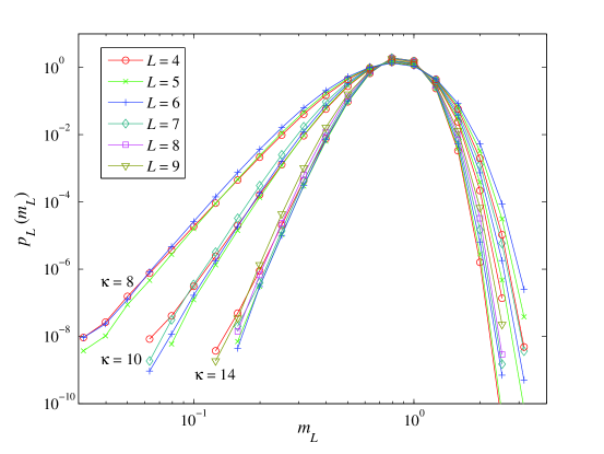
Figure 8: Log-log plot of the PDF of the coarse-grained mass $\bar{m}_{L}$ in one dimension for $p=2/3$ and various values of $\gamma$ and $L$ associated to three different ratios $\kappa=L/\log(1-\gamma/2)$ as labeled.

Such a rescaling is confirmed by numerical simulations. Figure 8 represents the PDF of the coarse-grained mass $\bar{m}_{L}$ for various values of $L$ and $\gamma$ chosen such that the ratio $\kappa$ is 8, 10 or 14. While the left-tail and the core of the distribution are clearly collapsing, the rescaling is much less evident for the right-hand tail. Obtaining better evidence would require much longer statistics in order to resolve the distribution at large masses.

6 Conclusions

We introduced here a simple model for the dynamics of heavy inertial particles in turbulent flow which solely accounts for their ejection from rotating structures of the fluid velocity field. We have shown that this model is able to reproduce qualitatively most features of the particle mass distribution which are observed in real turbulent flows. Namely the probability density of the mass in cells is shown to behave as a power-law at small arguments and to decrease faster than exponentially at large values. Moreover, we studied how this distribution depends on the parameters of the model, namely the ejection rate of particles from eddies and the fraction of space occupied by them. Such dependence reproduce again qualitatively observations from numerical simulations in homogeneous turbulent flows. Finally, we have seen that coarse-graining masses on scales larger than the cell size is asymptotically equivalent to decrease the ejection rate related to particle inertia. This gives evidence that there exists a scaling in the limit of large observation scale and small response time of the particles, even if the flow has no scale invariance.

There are several extensions that need to be investigated in order to gain from the study of such models a more quantitative information on the distribution of particles in real flows. The most significant improvement is to give a spatial structure to the fluid velocity. This can be done by introducing a spatial correlation between the vorticities of cells. Preliminary investigations suggest that such a modified model could be approached by taking its continuum limit. Another effect that may be worth taking into consideration is random sweeping of structures by the fluid flow. We assumed that the eddies are frozzen (and occupy the same cell) during their whole life time. The model could be extended by adding to the dynamics random hops between cells of these structures. Another extension could consist in investigating in a systematic manner three-dimensional versions of the model. As stated above, many statistical quantities may depend on how ejection from rotating regions is implemented in three dimensions. Finally, it is worth mentioning again that the main advantage of such models is to give a heuristic understanding of the relations between the properties of the fluid velocity field and the mass distribution of particles. This first step is necessary in the development of a phenomenological framework for describing the spatial distribution of heavy particles in turbulent flows. This would allow for using Kolmogorov 1941 dimensional arguments to understand how the particle dynamical properties depend on scale. Moreover, such a framework could be used to obtain refined predictions accounting for the effect of the fluid flow intermittency and to describe the dependence upon the Reynolds number of the spatial distribution of particles.

References

References

- [1] P. Dimotakis. Turbulent mixing. Ann. Rev. Fluid Mech., 37:329–356, 2005.
- [2] M.R. Maxey and J. Riley. Equation of motion of a small rigid sphere in a nonuniform flow. Phys. Fluids, 26:883–889, 1983.
- [3] J.K. Eaton and J.R. Fessler. Preferential concentration of particles by turbulence. Int. J. Multiphase Flow, 20:169–209, 1994.
- [4] G. Falkovich, A. Fouxon, and M. Stepanov. Acceleration of rain initiation by cloud turbulence. Nature, 419:151–154, 2002.
- [5] D. Lewis and T. Pedley. The influence of turbulence on plankton predation strategies. J. Theor. Biol., 210:347–365, 2001.
- [6] J. Seinfeld. Atmospheric chemistry and physics of air pollution. J. Wiley and sons, New York, 1986.
- [7] I. de Pater and J. Lissauer. Planetary Science. Cambridge University Press, Cambridge, 2001.
- [8] J. Bec. Multifractal concentrations of inertial particles in smooth random flow s. J. Fluid Mech., 528:255–277, 2005.
- [9] M.R. Maxey. The gravitational settling of aerosol particles in homogeneous turbulen ce and random flow fields. J. Fluid Mech., 174:441–465, 1987.
- [10] R.H. Kraichnan. Small-scale structure of a scalar field convected by turbulence. Phys. Fluids, 11:945–953, 1968.
- [11] L.I. Piterbarg. The top lyapunov exponent for stochastic flow modeling the upper ocean turbulence. SIAM J. Appl. Math., 62:777–800, 2002.
- [12] B. Mehlig and M. Wilkinson. Coagulation by random velocity fields as a kramers problem. Phys. Rev. Lett., 92:250602, 2004.
- [13] K. Duncan, B. Mehlig, S. Östlund, and M. Wilkinson. Clustering by mixing flows. Phys. Rev. Lett., 95:240602, 2005.
- [14] S. Derevyanko, G. Falkovich, K. Turitsyn, and S. Turitsyn. Explosive growth of inhomogeneities in the distribution of droplets in a turbulent air. Preprint nlin.CD/0602006, 2006.
- [15] J. Bec, M. Cencini, and R. Hillerbrand. Heavy particles in incompressible flows: the large stokes number asymptotics. Physica D, 226:11–22, 2007.
- [16] J. Bec, L. Biferale, M. Cencini, A. Lanotte, S. Musacchio, and F. Toschi. Time scales of particle clustering in turbulent flows. Preprint nlin.CD/0608045, 2006.