Universality in the flooding of regular islands by chaotic states

Abstract

We investigate the structure of eigenstates in systems with a mixed phase space in terms of their projection onto individual regular tori. Depending on dynamical tunneling rates and the Heisenberg time, regular states disappear and chaotic states flood the regular tori. For a quantitative understanding we introduce a random matrix model. The resulting statistical properties of eigenstates as a function of an effective coupling strength are in very good agreement with numerical results for a kicked system. We discuss the implications of these results for the applicability of the semiclassical eigenfunction hypothesis.

I Introduction

The classical dynamics in Hamiltonian systems shows a rich behaviour ranging from integrable to fully chaotic motion. In chaotic systems nearby trajectories separate exponentially in time and ergodicity implies that a typical trajectory fills out the energy-surface in a uniform way. However, integrable and fully chaotic dynamics are exceptional MarMey74 as typical Hamiltonian systems show a mixed phase space in which regions of regular motion, the so-called regular islands around stable periodic orbits, and chaotic dynamics, the so-called chaotic sea, coexist.

For quantized Hamiltonian systems the fundamental questions concern the behaviour of the eigenvalues and the properties of eigenfunctions, especially in the semiclassical regime. From the semiclassical eigenfunction hypothesis Per73 ; Vor76 ; Ber77b ; Vor79 ; Ber83 one expects that in the semiclassical limit the eigenstates concentrate on those regions in phase space which a typical orbit explores in the long-time limit. For integrable systems these are the invariant tori. In contrast, for ergodic systems almost all orbits fill the energy shell in a uniform way. For this situation the semiclassical eigenfunction hypothesis is proven by the quantum ergodicity theorem which shows that almost all eigenstates become equidistributed on the energy shell Qerg .

For systems with a mixed phase space, in the semiclassical limit $(h\rightarrow 0)$, the semiclassical eigenfunction hypothesis implies that the eigenstates can be classified as being either regular or chaotic according to the phase-space region on which they concentrate. This is supported by several studies, see e.g. BohTomUll93 ; ProRob93b ; LiRob95b ; CarVerFen98 ; VebRobLiu99 ; MarKee2005 . It is also possible, that the influence of a regular island quantum mechanically extends beyond the outermost invariant curve due to partial barriers like cantori and that quantization conditions remain approximately applicable even outside of the island BohTomUll93 . However, it was recently shown that the classification into regular and chaotic states does not hold when the phase space has an infinite volume HufKetOttSch2002 . In this case eigenstates may completely ignore the classical phase space boundaries between regular and chaotic regions.

In order to understand the behaviour of eigenstates away from the semiclassical limit, i.e. at finite values of the Planck constant $h$, one has to compare the size of phase-space structures with $h$. Let us consider for simplicity the case of two-dimensional area preserving maps and their quantizations. Regular states of an island concentrate on tori which fulfill the EBK-type quantization condition

$$\oint p\,\text{d}q=(m+1/2)h\qquad m=0,1,...$$ (1)

for the enclosed area BerBalTabVor79 . This quantization rule explicitly shows that regular eigenstates only appear if $h/2$ is smaller than the area $A_{\text{reg}}$ of that island.

Another consequence of finite $h$ in systems with a mixed phase space is dynamical tunneling DavHel81 , i.e. tunneling through dynamically generated barriers in phase space, in contrast to the usual tunneling under a potential barrier. Dynamical tunneling couples the subspace spanned by the regular basis states, corresponding to the quantization condition (1), with the complementary subspace ftn2 composed of chaotic basis states. This raises the question whether the eigenstates of such a quantum system can still be called regular or chaotic.

In Ref. BaeKetMon2005 it was shown that (1) is not a sufficient condition for the existence of a regular eigenstate on the $m$-th quantized torus. In addition one has to fulfill

$$\gamma_{m}<\frac{1}{\tau_{\text{\tiny{H,ch}}}},$$ (2)

where $\tau_{\text{\tiny{H,ch}}}=h/\Delta_{\text{ch}}$ is the Heisenberg time of the surrounding chaotic sea with mean level spacing $\Delta_{\text{ch}}$ and $\gamma_{m}$ is the decay rate of the $m$-th regular state, if the chaotic sea were infinite. When condition (2) is violated one observes eigenstates which extend over the chaotic region and flood the $m$-th torus BaeKetMon2005 . To distinguish them from the chaotic eigenstates that do not flood the torus, they are referred to as flooding eigenstates. For the limiting case of complete flooding of all tori, the corresponding eigenstates were called amphibious HufKetOttSch2002 . Recently, the consequences of flooding for the transport properties in rough nano-wires were studied FeiBaeKetRotHucBur2006 .

The process of flooding was explained and demonstrated for a kicked system in Ref. BaeKetMon2005 . Condition (2) was obtained by scaling arguments, which cannot provide a prefactor. Moreover, for an ensemble of systems, one would like to know the probability for the existence of a regular eigenstate. In particular, when varying the Heisenberg time, how broad is the transition regime during which this probability goes from 1 to 0? Another question is, how do the chaotic eigenstates turn into flooding eigenstates for a given torus?

In this paper we give quantitative answers to these questions. We study the flooding of regular tori in terms of the weight of eigenstates inside the regular region and devise a random matrix model which allows for describing the statistics of these weights in detail. Random matrix models have been very successful for obtaining quantitative predictions on eigenstates in both fully chaotic systems and systems with a mixed phase space, see e.g. KusMosHaa1988 ; BohTomUll93 ; HaaZyc1990 ; TomUll1994 ; Bae2003 ; KeaMezMon2003 . For the present situation we propose a random matrix model which takes regular basis states and their coupling to the chaotic basis states into account. The only free parameters are the strength of the coupling and the ratio of the number of regular to the number of chaotic basis states. From this model the weight distribution for eigenstates is determined.

For a kicked system we define the weight by the projection of the eigenstates onto regular basis states localized on a given torus $m$. The distribution of the weights allows for studying the flooding of each torus separately. The resulting distributions are compared with the prediction of the random matrix model and, after an appropriate rescaling, very good agreement is observed. This agreement shows explicitly the universal features underlying the process of flooding, giving a precise criterion for the existence or non–existence of regular, chaotic, and flooding eigenstates in mixed systems.

The text is organized as follows. In section II we introduce the kicked system used for the numerical illustrations, both classically (part A) and quantum mechanically (part B). In section II C we define the weight of an eigenstate by its projection onto regular basis states and investigate the distribution of the weights for the kicked system. In section III we introduce the random matrix model and determine the corresponding weight distribution as a function of the coupling strength. In section IV the relation between parameters of the kicked system and the random matrix model is derived. This allows for a direct comparison of the distributions. In section V we consider the fraction of regular eigenstates, both for an individual torus and for the entire island. In section VI we briefly discuss the consequences of the random matrix model on the number of flooding eigenstates. A summary and discussion of the eigenfunction structure in generic systems with a mixed phase space is given in section VII.

II The Kicked System

II.1 Classical dynamics

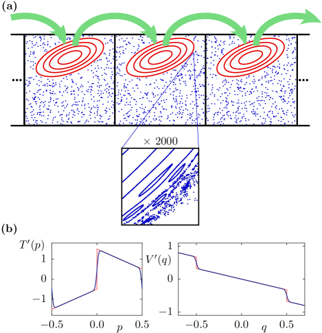
Figure 1: (color online) (a) Classical dynamics of the kicked system given by Eqs. (4) and (5). Invariant tori of the regular island are shown (continuous curves) and the transport to the right is indicated by the arrows. The dots correspond to one chaotic orbit. The magnification shows that the boundary of the island to the chaotic sea is rather sharp with only very small secondary islands. (b) Smoothed functions $T^{\prime}(p)$ and $V^{\prime}(q)$ (blue, dark lines) and discontinuous functions $t^{\prime}(p)$ and $v^{\prime}(q)$ (red, light lines) according to Eqs. (6-9).

For a general one-dimensional kicked Hamiltonian

$$H(p,q,t)=T(p)+V(q)\sum_{n=-\infty}^{\infty}\delta(t-n)\ ,$$ (3)

the dynamics is fully determined by the mapping of position and momentum $(q_{n},p_{n})$ at times $t=n+0^{+}$ just after the kicks

$$q_{n+1} = q_{n}+T^{\prime}(p_{n})\ ,$$ (4)

$$p_{n+1} = p_{n}-V^{\prime}(q_{n+1})\ .$$ (5)

Choosing the functions $T^{\prime}(p)$ and $V^{\prime}(q)$ appropriately, one can obtain a system with a large regular island and a homogeneous chaotic sea. For the system considered in BaeKetMon2005 , first introduced in HufKetOttSch2002 , one starts with the piecewise linear functions (see Fig. 1b)

$$t^{\prime}(p) = \frac{1}{2}+\left(\frac{1}{2}-sp\right){\rm sign}\left(p-\lfloor p+1/2\rfloor\right)\ ,$$ (6)

$$v^{\prime}(q) = -rq-(1-r)\lfloor q+1/2\rfloor\ ,$$ (7)

where $\lfloor x\rfloor$ is the floor function, and $s$ and $r$ are two parameters determining the properties of the regular island and the chaotic sea. Using a Gaussian smoothing with $G_{\varepsilon}(z)=\exp(-z^{2}/2\varepsilon^{2})/\sqrt{2\pi\varepsilon^{2}}$, one obtains analytic functions

$$T^{\prime}(p) = \int_{-\infty}^{\infty}\text{d}z\;t^{\prime}(p+z)\;G_{\varepsilon}(z)\ ,$$ (8)

$$V^{\prime}(q) = \int_{-\infty}^{\infty}\text{d}z\;v^{\prime}(q+z)\;G_{\varepsilon}(z)\ .$$ (9)

By construction, these functions have the periodicity properties

$$T^{\prime}(p+k) = T^{\prime}(p)\ ,$$ (10)

$$V^{\prime}(q+k) = V^{\prime}(q)-k\ ,$$ (11)

for any integer $k$. We consider $p\in[-1/2,1/2[$ and $q\in[-1/2,-1/2+M[\,$ with periodic boundary conditions. The phase space is composed of a chain of transporting islands centered at $(\bar{q},\bar{p})=(k,1/4)$ with $0\leq k\leq M-1$ that are mapped one unit cell to the right (see Fig. 1a). The surrounding chaotic sea has an average drift to the left as the overall transport is zero SchOttKetDit2001 ; SchDitKet2005 . The fine scale structure at the boundary of the island to the chaotic sea has a very small area (see the magnification in Fig. 1a). Resonances in this layer are irrelevant in the $h$ regime studied here. For $s=2$, $r=0.65$ and $\varepsilon=0.015$ the regular island has a relative area $A_{\text{reg}}\approx 0.215$.

II.2 Quantization

In kicked systems, the quantum evolution of a state after one period of time

$$|\psi(t+1)\rangle=\hat{U}|\psi(t)\rangle\ ,$$ (12)

is fully determined by the unitary operator, see e.g. BerBalTabVor79 ; HanBer80 ; ChaShi86 ; Esp93 ; DegGra03 ,

$$\hat{U}=\exp\left(-\frac{2\pi\text{i}}{h_{\text{eff}}}V(\hat{q})\right)\exp\left(-\frac{2\pi\text{i}}{h_{\text{eff}}}T(\hat{p})\right)\ .$$ (13)

Here the effective Planck’s constant $h_{\text{eff}}$ is Planck’s constant $h$ divided by the size of one unit cell. The eigenstates of this operator are defined by

$$\hat{U}|\psi_{j}\rangle=\text{e}^{2\pi\text{i}\varphi_{j}}|\psi_{j}\rangle\ ,$$ (14)

where the eigenphase $\varphi_{j}$ is the quasienergy divided by $\hbar\omega$. In order to fulfill the periodicity of the classical dynamics in $p$ direction, the quantum states have to obey the quasi-periodicity condition

$$\langle p+1|\psi\rangle=\text{e}^{-2\pi\text{i}\chi_{p}}\langle p|\psi\rangle\ .$$ (15)

One can show that this leads to quantum states that are a linear combination of the discretized position states $|q_{j}\rangle$, with $q_{j}=h_{\text{eff}}(j+\chi_{p})$. Additionally, imposing periodicity after $M$ unit cells in $q$ direction, quantum states have to fulfill the property

$$\langle q+M|\psi\rangle=\text{e}^{2\pi\text{i}\chi_{q}}\langle q|\psi\rangle\ .$$ (16)

Because of the required periodicity the phase space is compact and the effective Planck’s constant can only be a rational number

$$h_{\text{eff}}=\frac{M}{N}\ .$$ (17)

We consider the case of incommensurate $M$ and $N$, so that the quantum system is not effectively reduced to less than $M$ cells.

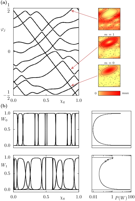
Figure 2: (color online) (a) Eigenphases of the kicked system vs $\chi_{q}$ for $h_{\text{eff}}=1/10$. The pattern of straight lines (interrupted by avoided crossings) with negative slope corresponds to regular eigenstates with $m=0$ and $m=1$ whose Husimi functions are shown to the right. The other eigenstates are chaotic and live outside of the regular region, as can be seen from the Husimi representation. (b) Weights $W_{0}$ and $W_{1}$ of all eigenstates vs $\chi_{q}$ (left). Distribution $P(W)$ of these weights in a log-linear representation (right).

The properties (10), (11) of $T^{\prime}(p)$ and $V^{\prime}(q)$ imply for their integrals

$$T(p+k) = T(p)\ ,$$ (18)

$$V(q+k) = V(q)-kq-\frac{k^{2}}{2}\ .$$ (19)

From this one finds that the propagator $\hat{U}$ is consistent with the periodicity conditions (15) and (16) if and only if

$$M\left(\chi_{p}+\frac{N}{2}\right)\in\mathbb{Z}\ .$$ (20)

For given $M$ and $N$, this condition limits the possible values of the phase $\chi_{p}$, while $\chi_{q}$ remains arbitrary. Thus, in the basis given by the position states $|q_{j}\rangle$, with $0\leq j\leq N-1$, where $N$ is the dimension of the Hilbert space, the propagator $\hat{U}$ is represented by the finite $N\times N$ unitary matrix

$$U_{kl}=\frac{1}{N}\sum_{j=0}^{N-1}\text{e}^{-\frac{\text{i}}{\hbar_{\text{eff}}}\left[V(q_{k})+T(p_{j})+p_{j}(q_{l}-q_{k})\right]}\ ,$$ (21)

where $0\leq k,l\leq N-1$ and $p_{j}=(j+\chi_{q})/N$. Finding the solution of (14), i.e. the eigenphases and eigenstates of the system, therefore reduces to the numerical diagonalization of the matrix (21). The result is illustrated in Fig. 2(a) for $h_{\text{eff}}=1/10$, where the eigenphases are plotted as a function of $\chi_{q}$. The straight lines with negative slope correspond to the regular eigenstates SchOttKetDit2001 ; SchDitKet2005 , whose Husimi distributions are shown to the right in Fig. 2(a). Lines with an average positive slope correspond to chaotic eigenstates.

When the system consists of $M$ unit cells one has $M$ regular basis states localized on the $m$-th torus. Their EBK eigenphases are equispaced with a distance $1/M$ Sch:PhD-BaeKetMonSch .

II.3 Projection onto regular basis states

In order to investigate the amount of flooding we use the projection of the eigenstates onto regular basis states of the island region. For the considered kicked system regular basis states can be constructed from harmonic oscillator eigenstates, as the invariant tori are accurately approximated by ellipses Sch:PhD-BaeKetMonSch . The expression for the $m$-th harmonic oscillator state, centered in a phase space point $(\bar{q},\bar{p})$, is

$$\langle q |\varphi^{m}_{\bar{q},\bar{p}}\rangle=\frac{1}{\sqrt{2^{m}m!}}\left(\tfrac{{\rm Re}~{}\sigma}{\pi\hbar_{\text{eff}}}\right)^{1/4}H_{m}\left(\sqrt{\tfrac{{\rm Re}~{}\sigma}{\hbar_{\text{eff}}}}(q-\bar{q})\right)$$

$$\times\exp\left(-\tfrac{\sigma}{2\hbar_{\text{eff}}}(q-\bar{q})^{2}+\tfrac{\text{i}}{\hbar_{\text{eff}}}\bar{p}(q-\bar{q}/2)\right)$$ (22)

where $H_{m}$ is the Hermite polynomial of degree $m$. The complex constant $\sigma$ takes into account the squeezing and rotation of the state. From the linearized map at the stable fixed point of the island one finds $\sigma=(\sqrt{351}-13\,\text{i})/40$.

For a chain with $M$ identical cells, a regular basis state is a linear combination of the harmonic oscillator states $|\varphi^{m}_{k,1/4}\rangle$, centered in the $k$-th island for $0\leq k\leq M-1$ and properly normalized and periodized in the $q$ and $p$ directions Sch:PhD-BaeKetMonSch . The subspace spanned by these $M$ regular basis states is the same as the one spanned by the $M$ harmonic oscillator states $|\varphi^{m}_{k,1/4}\rangle$. Therefore, we define the weight $W_{m}$ of a normalized state $|\Psi\rangle$ by its projection onto this subspace corresponding to the $m$-th quantized torus

$$W_{m}=\sum_{k=0}^{M-1}|\langle\Psi|\varphi^{m}_{k,1/4}\rangle|^{2}\ .$$ (23)

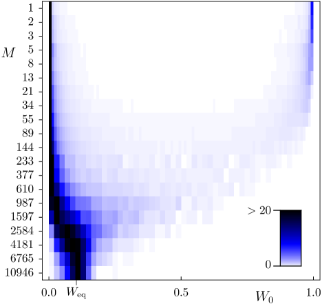
Figure 3: (color online) Distribution of $W_{0}$ (Eq. (23)) vs system size $M$ for effective Planck’s constant $h_{\text{eff}}\approx 1/10$.

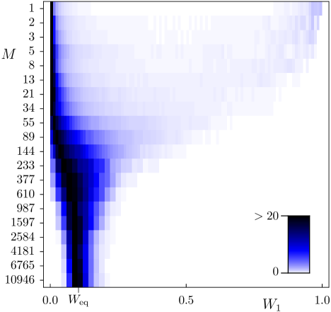
Figure 4: (color online) Distribution of $W_{1}$ (Eq. (23)) vs system size $M$ for effective Planck’s constant $h_{\text{eff}}\approx 1/10$.

By means of the weight $W_{m}$ for all eigenstates of Eq. (21) we can study the process of flooding for each torus separately. This allows for a detailed analysis and a quantitative comparison with a random matrix model. Therefore this is a considerable improvement compared to our previous analysis BaeKetMon2005 , where the weight was defined as the integral of the Husimi distribution of an eigenstate over the whole region of the island, which means that the information on individual tori is not accessible.

In Fig. 2(b) we show the weights $W_{0}$ and $W_{1}$ of all the eigenstates as a function of $\chi_{q}$. For $W_{0}$ we observe that for almost all $\chi_{q}$ the weights are essentially zero or one. Only at avoided crossings of regular and chaotic eigenstates their weights have intermediate values. For $m=1$ the avoided crossings are much broader due to the larger coupling and the value $W=1$ is not reached between several avoided crossings. This is also seen in the weight distributions shown to the right in Fig. 2(b), where the two peaks from the chaotic eigenstates (at $W=1$) and from the regular eigenstates (at $W=0$) are broader for $m=1$ in comparison with $m=0$. Note, that in the situation of isolated avoided crossings the involved eigenstates are often referred to as hybrid states.

The distribution of the weights $W_{m}$ allows for studying the process of flooding in a quantitative way. To violate condition (2) we need to increase the Heisenberg time, while keeping the tunneling rates $\gamma_{m}$ constant. We can achieve this by choosing a sequence of rational approximants $M/N$ of $h_{\text{eff}}=1/(d+g)$, with $d\in\mathbb{N}$ and the golden mean $g=(\sqrt{5}-1)/2\approx 0.618$. This ensures that, while the system size $M$ is increased, $h_{\text{eff}}$ is essentially kept at a fixed value, and therefore the tunneling rates $\gamma_{m}$ are independent of $M$. Simultaneously, the dimensionless Heisenberg time $\tau_{\text{\tiny{H,ch}}}=1/\Delta_{\text{ch}}$ increases linearly with $M$,

$$\tau_{\text{\tiny{H,ch}}}=N_{\text{ch}}=\left(\frac{1}{h_{\text{eff}}}-m_{\text{max}}\right)M\ ,$$ (24)

where we used $\Delta_{\text{ch}}=1/N_{\text{ch}}$ and $N_{\text{ch}}=N-m_{\text{max}}M$ is the number of chaotic states. Here $m_{\text{max}}$ is the maximal number of regular states in a single island according to the EBK quantization condition (1), $m_{\text{max}}=\left\lfloor A_{\text{reg}}/h_{\text{eff}}+1/2\right\rfloor$. As discussed in Ref. BaeKetMon2005 , $\tau_{\text{\tiny{H,ch}}}$ may be bounded, due to localization effects: For $M$ larger than the localization length $\lambda$ the effective mean level spacing $\Delta_{\text{ch}}\sim(\lambda N_{\text{ch}}/M)^{-1}$ leads to $\tau_{\text{\tiny{H,ch}}}\sim\lambda N_{\text{ch}}/M\approx\lambda h_{\text{eff}}$, where $\lambda$ is measured in multiples of a unit cell and $N_{\text{ch}}/M$ is the number of chaotic states per unit cell. For transporting islands, like in the model studied here, $\lambda\sim 1/\gamma_{0}$ is unusually large HanOttAnt1984 ; IomFisZas2002andrefs ; HufKetOttSch2002 , leading to a maximal value $\tau_{\text{\tiny{H,ch}}}\sim h_{\text{eff}}/\gamma_{0}$.

In Figs. 3 and 4 we show the distribution of $W_{0}$ and $W_{1}$ for $d=9$ (giving approximants $h_{\text{eff}}=1/10$, $2/19$, $3/29$, $5/48$, $\ldots$) for increasing system size $M$. For small system sizes we increased the statistics by varying the phase $\chi_{q}$ in the quantization, as it was shown in Fig. 2(b). To present the results in a compact form each histogram is shown using a color scale. The horizontal strips for $M=1$ in Fig. 3 and Fig. 4 correspond to the histograms previously shown in Fig. 2(b).

In Fig. 3 one clearly observes for small $M$ two separate peaks corresponding to chaotic eigenstates at $W=0$ ftn and regular eigenstates with $m=0$ at $W=1$. With increasing system size these regular eigenstates disappear while the weight $W_{0}$ of the chaotic eigenstates starts to increase and they turn into flooding eigenstates.

Comparing Fig. 4 for $W_{1}$ with Fig. 3 for $W_{0}$ one observes a qualitatively similar behavior. The difference is that the regular eigenstates with $m=1$ disappear for much smaller system size $M\approx 100$ than the eigenstates with $m=0$, as expected from Eq. (2) and their ratio of tunneling rates, $\gamma_{0}/\gamma_{1}\ll 1$.

For the largest values of $M$ only flooding eigenstates are left which fully extend over the chaotic sea and the regular island. The flooding is complete and the $N$ eigenstates are equally distributed in the Hilbert space. Projecting them onto the $M$ regular basis states leads to the average value $W_{\text{eq}}=M/N=h_{\text{eff}}\approx 1/10$, in agreement with the observed position of the peaks in Figs. 3 and 4 and the findings in Ref. HufKetOttSch2002 .

III Random Matrix Model

The similarity in the behavior of the histograms in Fig. 3 and Fig. 4, suggests a universality in the process of flooding, which should allow for a random matrix modelling. Such models have been used successfully for the case of mixed systems to describe the level splitting in the context of chaos assisted tunneling, see e.g. BohTomUll93 ; TomUll1994 ; LeyUll96 ; ZakDelBuc98 . In our case, we want to describe the statistics of eigenvectors for the situation of a chain of $N_{\text{reg}}$ regular islands. Here one has $N_{\text{reg}}$ equispaced regular levels corresponding to the $m$-th quantized torus and $N_{\text{ch}}$ COE distributed chaotic levels coupled by dynamical tunneling, see Fig. 5. For this situation we propose a random matrix model with the following block structure

$$H=\left(\begin{array}[]{c|c}\raisebox{0.0pt}[14.22636pt][8.53581pt]{\makebox[30.1388pt]{$H_{\rm reg}$}}&\raisebox{0.0pt}[14.22636pt][8.53581pt]{\makebox[30.1388pt]{$V$}}\\[0.86108pt] \hline\cr\raisebox{0.0pt}[14.22636pt][8.53581pt]{\makebox[30.1388pt]{$V^{T}$}}&\raisebox{0.0pt}[14.22636pt][8.53581pt]{\makebox[30.1388pt]{$H_{\rm ch}$}}\end{array}\right)\ .$$ (25)

This matrix is chosen to be real symmetric because the kicked system under consideration obeys time reversal symmetry. As a consequence of the block structure, the free parameters of this model are the ratio $N_{\text{reg}}/N_{\text{ch}}$ of the number of regular and chaotic basis states and the strength $v$ of the coupling.

Figure 5: Schematical plot of the regular levels with spacing $\Delta_{\text{reg}}$ coupled with strength $v\Delta_{\text{ch}}$ to the COE distributed chaotic levels with mean spacing $\Delta_{\text{ch}}$.

The first block $H_{\rm reg}$ models the regular basis states associated with one specific torus, while for simplicity we neglect the regular basis states quantized on other tori. As discussed at the end of Sec. II B, in the considered kicked system, the EBK eigenphases of the $N_{\text{reg}}$ regular basis states are equispaced. To mimic this behavior we consider for $H_{\rm reg}$ a diagonal matrix with elements $(k+\chi)/N_{\text{reg}}$, $k=0,1,\ldots,N_{\text{reg}}-1$. The parameter $\chi$ can be chosen from a uniform distribution between zero and one. The energies lie in the interval [0,1] with fixed spacing $\Delta_{\text{reg}}=1/N_{\text{reg}}$.

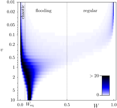
Figure 6: (color online) Distribution of weights in the random matrix model vs coupling strength $v$. The ratio $N_{\text{reg}}/N_{\text{ch}}$ approximates the value $1/(8+g)$. The dashed lines at $W=0.5$ and $W=0.5W_{\text{eq}}\approx 0.052$ separate chaotic, flooding, and regular eigenstates.

The block $H_{\rm ch}$ models the $N_{\text{ch}}$ chaotic basis states, where we assume $N_{\text{ch}}>N_{\text{reg}}$. It is also a diagonal matrix whose elements $\{E_{l}\}$ are the eigenphases of an $N_{\text{ch}}\times N_{\text{ch}}$ matrix of the Circular Orthogonal Ensemble (COE). These energies $\{E_{l}\}$ lie in the interval [0,1] with a uniform average density and show the typical level repulsion of chaotic systems. The mean level spacing of these basis states is $\Delta_{\text{ch}}=1/N_{\text{ch}}$. Note, that a GOE matrix for this block would have been less convenient as it leads to a non-uniform density of levels according to Wigner’s semicircle law.

The off-diagonal block $V$ accounts for the coupling between the regular and chaotic basis states. It is a $N_{\text{reg}}\times N_{\text{ch}}$ rectangular matrix, where each element is a random Gaussian variable with zero mean and variance $(v\Delta_{\text{ch}})^{2}$. The positive parameter $v$ is the coupling strength in units of the chaotic mean level spacing $\Delta_{\text{ch}}$. Thereby the results become asymptotically independent of the dimension $N_{\text{tot}}=N_{\text{reg}}+N_{\text{ch}}$ of the matrix for fixed $v$ and $N_{\text{reg}}/N_{\text{ch}}$.

We identify the regular region with the subspace spanned by the first $N_{\text{reg}}$ components. Therefore, for any normalized vector $(\Psi_{0},\ldots,\Psi_{N_{\text{reg}}-1},\Psi_{N_{\text{reg}}},\ldots,\Psi_{N_{\text{tot}}-1})$ we define the weight $W$ inside the regular region as

$$W=\sum_{j=0}^{N_{\text{reg}}-1}|\Psi_{j}|^{2}\ .$$ (26)

For a particular realization of the ensemble through the numbers $\{E_{l}\}$, $\chi$, and the block $V$, we compute the weights $W$ of the eigenvectors. We take for the statistics only those eigenvectors whose eigenenergies are in the interval [0.1, 0.9] to avoid possible border effects. We determine the distribution of $W$ by averaging over many different realizations. Increasing the matrix size $N_{\text{tot}}$ for a fixed ratio $N_{\text{reg}}/N_{\text{ch}}$ we find that the distribution converges. Considering a ratio $N_{\text{reg}}/N_{\text{ch}}=1/(8+g)$ and a small coupling strength $v\approx 0.1$ the distribution converges around $N_{\text{tot}}=200$. For $v\approx 1$ bigger matrices of $N_{\text{tot}}\approx 1000$ are necessary. For $v\approx 10$, we used $N_{\text{tot}}\approx 10000$. The limiting distributions depend sensitively on the coupling strength $v$.

In Fig. 6 we plot the distribution of $W$ for different values of $v$. We have to distinguish between the uncoupled regular and chaotic basis states of our model and the resulting eigenstates in the presence of the coupling. The eigenstates fall into three classes: a) Regular eigenstates ($W>0.5$), which predominantly live in the regular subspace. The remaining states, which predominantly live in the chaotic subspace, are divided into two classes, depending on the strength of their projection onto the regular subspace compared to the equilibrium value $W_{\text{eq}}=N_{\text{reg}}/N_{\text{tot}}$. This leads to b) flooding eigenstates ($0.5W_{\text{eq}}<W<0.5$), and c) chaotic eigenstates ($W<0.5W_{\text{eq}}$). Note, that the constants 0.5 in these definitions are arbitrary.

From the energy scales in the random matrix model, see Fig. 5, we expect three qualitatively different situations for the distribution of $W$:

i) $v\ll 1$, regular and chaotic eigenstates: In this regime the regular and chaotic blocks are practically decoupled as the coupling $v\Delta_{\text{ch}}$ is much smaller than the mean spacing of the chaotic basis states, $v\Delta_{\text{ch}}\ll\Delta_{\text{ch}}$. Two sharp peaks are observable, one at $W\approx 0$ due to the chaotic eigenstates, and the other at $W\approx 1$ due to the regular eigenstates. The latter peak has a smaller weight as the density of regular basis states is smaller.

ii) $v\approx 1$, chaotic and flooding eigenstates: Here the coupling $v\Delta_{\text{ch}}$ is approximately of the same order as the mean chaotic spacing $\Delta_{\text{ch}}$. All regular basis states are strongly coupled to several chaotic basis states and none of the eigenstates is predominantly regular. On the other hand one has different types of eigenstates as $v\Delta_{\text{ch}}<\Delta_{\text{reg}}$: Chaotic basis states, which are close in energy to a regular basis state, strongly couple and thus turn into flooding eigenstates. In contrast, there are many chaotic basis states which are far away from any regular basis state and only couple weakly. These lead to chaotic eigenstates which show essentially no flooding ($W<0.5W_{\text{eq}}$).

iii) $v\gg N_{\text{ch}}/N_{\text{reg}}$, flooding eigenstates: All chaotic basis states are strongly coupled to the regular basis states, $v\Delta_{\text{ch}}\gg\Delta_{\text{reg}}$. The resulting eigenstates equally flood the regular subspace. The distribution of $W$ gets a Gaussian shape with mean value $W_{\text{eq}}=N_{\text{reg}}/N_{\text{tot}}$ and a decreasing width.

In the transition from situation i) to ii) the two peaks of $P(W)$ near $W=0$ and $W=1$ broaden and move to the center. The regular peak broadens faster, and at $v\approx 0.25$ its maximum disappears. At $v\approx 1$ practically no eigenstates are localized in the regular subspace. When moving from situation ii) to iii) the different types of chaotic and flooding eigenstates transform into a single type of flooding eigenstates with a similar weight $W=W_{\text{eq}}$ in the regular subspace.

How do the resulting distributions depend on the ratio $N_{\text{reg}}/N_{\text{ch}}$? First, the average of $P(W)$ is given by $W_{\text{eq}}=N_{\text{reg}}/N_{\text{tot}}=1/(1+N_{\text{ch}}/N_{\text{reg}})$. Secondly, the regular peak in situation i) is independent of $N_{\text{reg}}/N_{\text{ch}}$ apart from a trivial scaling of the normalization with $N_{\text{reg}}/N_{\text{ch}}$. Numerically we checked that this is even true up to $v\approx 1$ for the distribution with $W>0.5$ and $N_{\text{reg}}/N_{\text{ch}}\leq 1/(8+g)$. Decreasing $N_{\text{reg}}/N_{\text{ch}}$ enlarges the size of the transition regime between ii) and iii). In particular, the peak near $W=0$ should stay there up to larger values of $v$.

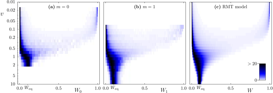
Figure 7: (color online) Distributions of the weights (a) $W_{0}$ and (b) $W_{1}$, taken from Figs. 3 and 4, with $M$ rescaled to $v$ according to (29). (c) Result for the random matrix (RMT) model from Fig. 6 on the same scale for a better comparison.

IV Comparison

The distribution of weights for the random matrix model, Fig. 6, shows a clear similarity to the results obtained for the kicked system, Figs. 3 and 4. In order to obtain a quantitative comparison one has to determine the relation between the coupling strength $v$ of the random matrix model and the system size $M$ of the kicked system. This can be deduced from Fermi’s golden rule in dimensionless form

$$\gamma=(2\pi)^{2}\frac{\langle V^{2}\rangle}{\Delta}\ ,$$ (27)

where the decay rate $\gamma$ of a regular state to a continuum of states with mean level spacing $\Delta$ is given by the variance of the coupling matrix elements $V$. In the random matrix model we have $\langle V^{2}\rangle=(v\Delta_{\text{ch}})^{2}$, $\Delta=\Delta_{\text{ch}}=1/N_{\text{ch}}$, and therefore (27) implies

$$v=\frac{\sqrt{\gamma N_{\text{ch}}}}{2\pi}\ .$$ (28)

Applying this relation to the kicked system, we first note that the tunnelling rate $\gamma_{m}$ for each torus can be determined numerically Sch:PhD-BaeKetMonSch (for recent theoretical results see OniShuIkeTak2001 ; BroSchUll2002 ; PodNar2003 ; EltSch2005 ; SchEltUll2005:p ; SheFisGuaReb2006 ). The determination of the correct value $N_{\text{ch}}$ for the kicked system requires a detailed discussion: A regular basis state on the $m$-th torus, in the case where the tori $m^{*},m^{*}+1,...,m_{\text{max}}-1$ are already flooded, will couple effectively to $N-m^{*}M$ states for $h_{\text{eff}}=M/N$. A change of $m^{*}$ affects $N_{\text{ch}}$ and therefore $v$. This dependence, however, can be neglected for the numerical comparison in our case: The ratio of the maximal and minimal possible values of $v$ is approximately $\sqrt{(1-h_{\text{eff}})/(1-A_{\text{reg}})}$. For $h_{\text{eff}}\approx 1/10$ and $A_{\text{reg}}=0.215$ this gives a difference of less than 7%. Therefore we simply use the maximal value $N_{\text{ch}}=N-M$ in the following.

For these values of $\gamma$ and $N_{\text{ch}}$ in Eq. (28) the $m$-th torus of the kicked system has a coupling strength

$$v=\frac{\sqrt{\gamma_{m}(1/h_{\text{eff}}-1)}}{2\pi}\sqrt{M}\ .$$ (29)

This allows for rescaling the results of the kicked system shown in Figs. 3 and 4 from $M$ to $v$ using the values $\gamma_{0}=0.0015$ and $\gamma_{1}=0.030$ Sch:PhD-BaeKetMonSch . The comparison with the results from the random matrix model is shown in Fig. 7. The agreement is very good for both tori over a wide range of coupling strengths $v$ showing the universality of the flooding process. For $v>5$, however, the distribution reaches a constant width in Fig. 7(b), while the variance decreases for the random matrix model, Fig. 7(c). We attribute this discrepancy to the localization of eigenstates in the kicked system for $M>1000$ HufKetOttSch2002 . As a consequence, the effective number of chaotic basis states near an island saturates (see the discussion after Eq. (24)), leading to an effective saturation of $v$.

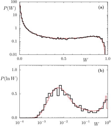
Figure 8: (color online) Distribution of (a) $W_{0}$ and (b) $\ln W_{0}$ for $h_{\text{eff}}=144/1385$ (dark lines). Results of random matrix model for $v=0.218$ and $N_{\text{reg}}/N_{\text{ch}}=1/8.618$ (light lines).

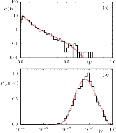
Figure 9: (color online) Distribution of (a) $W_{0}$ and (b) $\ln W_{0}$ for $h_{\text{eff}}=1597/15360$ (dark lines). Results of random matrix model for $v=0.726$ and $N_{\text{reg}}/N_{\text{ch}}=1/8.618$ (light lines).

In Figs. 8 and 9 we compare individual histograms for the weights $W_{0}$ for $m=0$. To visualize the low values of the distributions we choose a logarithmic-linear representation in Figs. 8(a) and 9(a). For $M=144$ one can distinguish the peak near $W=0$, due to chaotic eigenstates, from the second peak caused by regular eigenstates. For $M=1597$ these two peaks have merged and only a very small fraction of regular eigenstates is left. In both cases the distributions agree very well with the prediction of the random matrix model using $v$ according to Eq. (29). To resolve the peak near $W=0$ we show in Figs. 8(b) and 9(b) the distributions of $\ln W_{0}$. Again very good agreement with the predictions of the random matrix model is observed.

Fig. 10 shows the distribution of $\ln W_{1}$ for $m=1$ of all eigenstates for $h_{\text{eff}}=13/125$. We observe discrepancies at weights smaller than $10^{-3}$ in comparison to the random matrix model. This difference can be explained as follows: Among all the eigenstates of the kicked system there are regular eigenstates localized on the torus $m=0$ which are not considered in the random matrix model for $m=1$. These eigenstates have a negligible overlap with the regular basis states with $m=1$ because they are practically decoupled and only influence the histogram at very small weights. This is confirmed by computing the distribution, under exclusion of all eigenstates with $W_{0}>0.5$. The resulting distribution matches remarkably well with the prediction of our random matrix model.

Figure 10: (color online) Distribution of $\ln W_{1}$ of all eigenstates (thin line) for $h_{\text{eff}}=13/125$. After excluding states with $W_{0}>0.5$ (blue, dark line) much better agreement with the random matrix model (red, light line) is found.

V Fraction of regular eigenstates

A more global quantity than the individual distributions $P(W)$ is the fraction of regular eigenstates. This has been studied in Ref. BaeKetMon2005 for the total number of regular eigenstates as a function of the system size. With the projection onto individual regular basis states we are now able to study this fraction for each torus $m$ separately. For the kicked system with $M$ cells there are at most $M$ regular eigenstates localized on the $m$-th torus. However, during the process of flooding, some of these eigenstates disappear. Thus, we define the fraction $f_{\text{reg}}$ of regular eigenstates on the $m$-th torus as the number of eigenstates with weight $W_{m}>0.5$ divided by $M$. For small system sizes this fraction is averaged over several different phases $\chi_{q}$. To compare the resulting dependence on $M$ for different values of $m$ and $h_{\text{eff}}$ we determine the coupling strength $v$ using Eq. (29). These results are shown in Fig. 11.

For the random matrix model we compute $f_{\text{reg}}$ as the number of eigenstates with $W>0.5$ divided by the number of regular basis states $N_{\text{reg}}$, averaged over many realizations of the ensemble. As discussed at the end of section III, the distribution $P(W)$ for $W>0.5$ is independent of $N_{\text{reg}}/N_{\text{ch}}$, apart from a trivial rescaling. Therefore the resulting curve $f_{\text{reg}}(v)$ is independent of the ratio $N_{\text{reg}}/N_{\text{ch}}$ in contrast to the individual distributions. The agreement of the fractions determined for the kicked system with the random matrix curve in Fig. 11 is very good. This shows that $f_{\text{reg}}(v)$ is a universal curve describing the disappearance of regular eigenstates. For $v\leq 0.1$ the fraction of regular eigenstates is larger than 98%. For $v\geq 1$ the fraction of regular eigenstates is less than 1% and the corresponding regular torus is completely flooded.

Figure 11: (color online) Fraction of regular states $f_{\text{reg}}$ vs coupling strength $v$ for random matrix model (full line) and kicked system for various $h_{\text{eff}}$ and $m$ (symbols), where the system size $M$ is rescaled to $v$ according to Eq. (29). Fraction of flooding eigenstates $f_{\text{{f}l}}(v)$ for the random matrix model (dashed line) for $N_{\text{reg}}/N_{\text{ch}}=1/(8+g)$ showing a broader transition.

The criterion (2) for the existence of a regular eigenstate, expressed in terms of tunneling rate and Heisenberg time, can be transformed using Eqs. (28) and (24), into the condition

$$v<\frac{1}{2\pi}\;\;.$$ (30)

The position of $v=1/(2\pi)$ is indicated in Fig. 11 and roughly corresponds to 93% of regular eigenstates still existing (by the $W>0.5$ criterion). While in Ref. BaeKetMon2005 condition (2) for the existence of regular eigenstates was obtained from a scaling argument which does not provide a prefactor, our random matrix model analysis shows that it is quite close to 1.

For the transition regime $1/2\pi<v<1$ this model shows a decreasing probability for the existence of a regular eigenstate. For $v>1$, which implies

$$\gamma_{m}>(2\pi)^{2}\frac{1}{\tau_{\text{\tiny{H,ch}}}},$$ (31)

we find that almost no regular eigenstate exists on the $m$-th torus. Thus $v=1$ defines a critical system size $M_{m}$ associated with each quantized torus

$$M_{m}=\frac{4\pi^{2}h_{\text{eff}}}{\gamma_{m}(1-h_{\text{eff}})}\ .$$ (32)

With the knowledge about the flooding of individual tori we can now consider the total fraction of regular eigenstates. The regular tori with larger $m$ have typically a larger tunneling rate, $\gamma_{0}\ll\gamma_{1}\ll\ldots\ll\gamma_{m_{\text{max}}-1}$. Therefore the flooding of the regular tori happens sequentially from the outside of the island as the system size increases, as found in BaeKetMon2005 . The total fraction of regular eigenstates ${\cal F}_{\text{reg}}$ is defined as the number of eigenstates with weights $W_{m}>0.5$ for any $m$, divided by the total number of eigenstates $N$. With Eq. (32) we get the prediction

$${\cal F}_{\text{reg}}(M) = \frac{M}{N}\sum_{m=0}^{m_{\text{max}}-1}f_{\text{reg}}\left(\sqrt{\frac{M}{M_{m}}}\ \right)\ ,$$ (33)

where $f_{\text{reg}}(v)$ is the universal curve from the random matrix model. For small system sizes $M<M_{m}$ for all $m$ the total fraction of regular eigenstates is ${\cal F}_{\text{reg}}(M)=Mm_{\text{max}}/N\approx A_{\text{reg}}$, as expected from the semiclassical eigenfunction hypothesis. Fig. 12 shows ${\cal F}_{\text{reg}}(M)$ with a succession of plateaus and drops before each critical size $M_{m}$. Considering that the ratio of successive $M_{m}$ only varies moderately, the overall behavior of ${\cal F}_{\text{reg}}$ is an approximately linear decrease on a logarithmic scale in $M$, explaining the observations of Ref. BaeKetMon2005 . The agreement of Eq. (33) with the fraction of regular eigenstates for the kicked system for different $h_{\text{eff}}$ as seen in Fig. 12 is remarkably good.

We conclude this section with the remark that due to the independence of $f_{\text{reg}}(v)$ on the ratio $N_{\text{reg}}/N_{\text{ch}}$ one can obtain this universal curve by considering a simpler random matrix model, where only one regular basis state is coupled to an infinite number of chaotic basis states LeyUll96 . For this simpler model it might be possible to obtain analytical expressions for $f_{\text{reg}}(v)$.

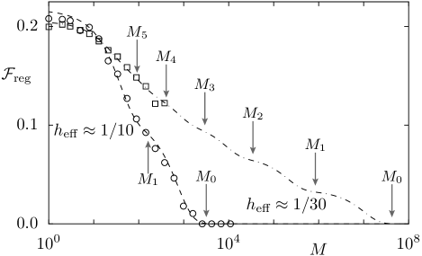
Figure 12: Total fraction of regular states ${\cal F}_{\text{reg}}$ vs system size $M$ according to the prediction Eq. (33), (lines) in agreement with the data for the kicked system for $h_{\text{eff}}\approx 1/10$ (circles) and $h_{\text{eff}}\approx 1/30$ (squares). The arrows indicate the critical system sizes $M_{m}$ according to Eq. (32).

VI Fraction of flooding eigenstates

The random matrix model also allows for investigating the fraction of flooding eigenstates. While the regular eigenstates disappear with increasing coupling strength $v$, more eigenstates turn into flooding eigenstates with $0.5W_{\text{eq}}<W<0.5$. Fig. 11 shows the increasing fraction of these states for the random matrix model with $N_{\text{reg}}/N_{\text{ch}}=1/(8+g)$. Note, that this fraction is defined as the number of flooding eigenstates divided by the number $N_{\text{tot}}$ of all eigenstates. At $v=1$ all regular eigenstates have disappeared, however, the fraction of flooding eigenstates is just 70%. The remaining eigenstates are chaotic, which have no substantial weight in the regular subspace. For larger values of $v$ they turn into flooding eigenstates. This roughly happens when each chaotic basis state is coupled to at least one regular basis state, i.e. when $v\Delta_{\text{ch}}=\Delta_{\text{reg}}/2$, see Fig. 5. This gives $v=N_{\text{ch}}/(2N_{\text{reg}})\approx 4.8$ which is in good agreement with the saturation observed in Fig. 11. This shows that the fraction of flooding eigenstates explicitly depends on the parameter $N_{\text{reg}}/N_{\text{ch}}$ in contrast to the fraction of regular states $f_{\text{reg}}(v)$.

Applying this result of the random matrix model to the kicked system where $v=N_{\text{ch}}/(2N_{\text{reg}})\approx N/(2M)$, we find using Eqs. (28) and (24), that the fraction of flooding eigenstates is saturated at $f_{\text{{f}l}}=1$ for

$$\gamma_{m}>\left(\frac{\pi}{h_{\text{eff}}}\right)^{2}\frac{1}{\tau_{\text{\tiny{H,ch}}}}$$ (34)

Note, that this prefactor increases in the semiclassial limit leading to a broader transition to flooding eigenstates.

VII Summary and discussion

We provide a detailed quantitative description of the flooding of regular islands. By using the projection of eigenstates onto regular basis states, which defines the weights $W_{m}$, the process of flooding can be described separately for each torus. The distribution of these weights in the kicked system agrees accurately with the distribution obtained by the proposed random matrix model. This model depends on two parameters only: the coupling strength $v$ between regular and chaotic basis states and the ratio of the number of those states $N_{\text{reg}}/N_{\text{ch}}$. The connection of this coupling strength with the parameters of the kicked system is given by Eq. (29).

From the random matrix model we gain the following general insights into the flooding of the $m$-th torus in terms of its tunneling rate $\gamma_{m}$ and the Heisenberg time $\tau_{\text{\tiny{H,ch}}}$:

i) $\gamma_{m}<\frac{1}{\tau_{\text{\tiny{H,ch}}}}$: All regular eigenstates on the $m$-th torus exist. None of the eigenstates predominantly extending over the chaotic region has substantially flooded the $m$-th torus.

ii) $\gamma_{m}=(2\pi)^{2}\frac{1}{\tau_{\text{\tiny{H,ch}}}}$: No regular eigenstates on the $m$-th torus exist. Some of the eigenstates predominantly extending over the chaotic region have substantially flooded the $m$-th torus.

iii) $\gamma_{m}>\left(\frac{\pi}{h_{\text{eff}}}\right)^{2}\frac{1}{\tau_{\text{\tiny{H,ch}}}}$: All of the eigenstates predominantly extending over the chaotic region have substantially flooded the $m$-th torus.

What do these results imply for the applicability of the semiclassical eigenfunction hypothesis? For a fixed system size in the semiclassical limit $h_{\text{eff}}\rightarrow 0$, which implies a roughly exponential decrease of $\gamma_{m}$, one ends up in regime i), in agreement with the semiclassical eigenfunction hypothesis. In contrast, for small $h_{\text{eff}}\neq 0$ fixed and systems with $M$ cells and $M\to\infty$, one obtains a large value for $\tau_{\text{\tiny{H,ch}}}\propto M$, limited by dynamical localization only. Depending on the localization length one ends up in regime iii) for some or all tori $m$. As in our case one has $\tau_{\text{\tiny{H,ch}}}\sim h_{\text{eff}}/\gamma_{0}$, regime iii) is realized for all tori, i.e. complete flooding of the island HufKetOttSch2002 .

The universality in the transition from i) to ii) can be seen for the fraction of regular states $f_{\text{reg}}(v)$ localized on a given torus. For the random matrix model this fraction does not depend on the ratio $N_{\text{reg}}/N_{\text{ch}}$ and the agreement with the results for the kicked system is remarkably good for different quantized tori and values of $h_{\text{eff}}$. In contrast to the disappearance of regular eigenstates on the $m$-th torus, the transition to flooding eigenstates on this torus is much broader and extends to regime iii).

It is also important to discuss, what these results imply for the case of a single island in a chaotic sea ($M=1$). Most commonly one is in regime i), i.e. regular and chaotic eigenstates exist and only mix at accidental avoided crossings. For a sufficiently small island, compared to the size of the chaotic region, regime ii) can be reached. Here $h_{\text{eff}}$ is small enough to quantum mechanically resolve the small regular island, but a corresponding regular state does not exist. It is not possible, however, to get into regime iii) where all eigenstates would be flooding eigenstates: In Eq. (34) we have $h_{\text{eff}}=1/N$ and $\tau_{\text{\tiny{H,ch}}}=N_{\text{ch}}\approx N$ such that the right hand side is approximately $\pi^{2}N$, which is always larger than the tunneling rates $\gamma_{m}<1$.

In the case of an island chain of period $p$ embedded in a chaotic sea it might be possible to get into regime iii): In the derivation of Eq. (34) we now have to use $v=N_{\text{ch}}/(2N_{\text{reg}})\approx N/(2p)=1/(2ph_{\text{eff}})$, leading with Eqs. (28) and $N_{\text{ch}}\approx N=1/h_{\text{eff}}$ to $\gamma>\pi^{2}/(p^{2}h_{\text{eff}})$. The right hand side can be smaller than 1 if $p$ is sufficiently large while $h_{\text{eff}}$ is small enough to resolve the individual islands of the chain. Whether this is indeed possible in typical systems requires further investigations.

This discussion shows that the semiclassical limit in generic systems with a mixed phase space, where islands of arbitrarily small size exist, is rather complicated. For example one can ask how small does $h_{\text{eff}}$ have to be such that at least one regular state exists on a small island of size $A_{\text{reg}}$? Let us define the ratio $r=h_{\text{eff}}/A_{\text{reg}}$ The quantization condition Eq. (1) implies that $r<2$ is necessary to quantum mechanically resolve the island. However, we find that the necessary ratio $r$ becomes arbitrarily small for small islands: Regime i) for $m=0$ requires $\gamma_{0}<1/\tau_{\text{\tiny{H,ch}}}\approx h_{\text{eff}}$. The tunneling rate $\gamma_{0}$ is an approximately exponentially decreasing function $\gamma_{0}\sim\exp(-C/r)$ with $C$ of the order of 1 HanOttAnt1984 ; FeiBaeKetRotHucBur2006 . Thus we have to fulfill $\exp(-C/r)/r<A_{\text{reg}}$, which for decreasing $A_{\text{reg}}$ is only possible if $r$ is sufficiently small.

We conclude by emphasizing that the universality given by the random matrix model not only holds for the kicked system studied here, but is applicable to any system with a mixed phase space. The consequences for the semiclassical limit in the hierarchical phase–space structure of generic systems needs much further investigation.

Acknowledgements

We thank S. Tomsovic, D. Ullmo and H. Weidenmüller for useful discussions, Lars Schilling for providing us with the data for the tunneling rates, and the Deutsche Forschungsgemeinschaft for support under contract KE 537/3-2.

References

- (1) L. Markus and K. Meyer, Generic Hamiltonian Dynamical Systems are neither Integrable nor Chaotic, no. 114 in Mem. Amer. Math. Soc. (American Mathematical Society, Providence, Rhode Island, 1974).
- (2) I. C. Percival, J. Phys. B 6, L229 (1973).
- (3) A. Voros, Annales de l’Institut Henri Poincaré A 24, 31 (1976).
- (4) M. V. Berry, J. Phys. A 10, 2083 (1977).
- (5) A. Voros, in Stochastic Behavior in Classical and Quantum Hamiltonian Systems, no. 93 in Lecture Notes in Physics, pages 326–333 (Springer-Verlag, Berlin, 1979).
- (6) M. V. Berry, in G. Iooss, R. H. G. Hellemann and R. Stora (eds.), Comportement Chaotique des Systèmes Déterministes — Chaotic Behaviour of Deterministic Systems, pages 171–271 (North-Holland, Amsterdam, 1983).
- (7) A. I. Shnirelman, Usp. Math. Nauk 29 (1974) 181; S. Zelditch, Duke. Math. J. 55 (1987) 919; Y. Colin de Verdière, Commun. Math. Phys. 102 (1985) 497; B. Helffer, A. Martinez and D. Robert, Commun. Math. Phys. 109 (1987) 313; P. Gérard and E. Leichtnam, Duke Math. J. 71 (1993) 559; S. Zelditch and M. Zworski, Commun. Math. Phys. 175 (1996) 673; A. Bouzouina and S. De Biévre, Commun. Math. Phys. 178 (1996) 83; S. De Bièvre and M. Degli Esposti, Ann. Inst. Henri Poincaré, Physique Théorique 69 (1996) 1; for an introduction see A. Bäcker, R. Schubert and P. Stifter, Phys. Rev. E 57 (1998) 5425.
- (8) O. Bohigas, S. Tomsovic and D. Ullmo, Phys. Rep. 223, 43 (1993).
- (9) T. Prosen and M. Robnik, J. Phys. A 26, 5365 (1993).
- (10) B. Li and M. Robnik, J. Phys. A 28, 4843 (1995).
- (11) G. Carlo, E. Vergini and A. J. Fendrik, Phys. Rev. E 57, 5397 (1998).
- (12) G. Veble, M. Robnik and J. Liu, J. Phys. A 32, 6423 (1999).
- (13) J. Marklof and S. O’Keefe, Nonlinearity 18, 277 (2005).
- (14) L. Hufnagel, R. Ketzmerick, M.-F. Otto and H. Schanz, Phys. Rev. Lett. 89, 154101 (2002).
- (15) M. V. Berry, N. L. Balazs, M. Tabor and A. Voros, Ann. Phys. 122, 26 (1979).
- (16) M. J. Davis and E. J. Heller, J. Chem. Phys. 75, 246 (1981).
- (17) Whether these subspaces are orthogonal or only approximately orthogonal has no consequences for the present work and for simplicity we assume orthogonality, as e.g. in Ref. BohTomUll93 .
- (18) A. Bäcker, R. Ketzmerick and A. G. Monastra, Phys. Rev. Lett. 94, 054102 (2005).
- (19) J. Feist, A. Bäcker, R. Ketzmerick, S. Rotter, B. Huckestein and J. Burgdörfer, Phys. Rev. Lett. 97, 116804 (2006).
- (20) M. Kuś, J. Mostowski and F. Haake, J. Phys. A 21, L1073 (1988).
- (21) F. Haake and K. Życzkowski, Phys. Rev. A 42, 1013 (1990).
- (22) S. Tomsovic and D. Ullmo, Phys. Rev. E 50, 145 (1994).
- (23) A. Bäcker, in: The Mathematical Aspects of Quantum Maps, M. Degli Esposti and S. Graffi (Eds.), Springer Lecture Notes in Physics 618, 91 (2003).
- (24) J. P. Keating, F. Mezzadri and A. G. Monastra, J. Phys. A 36, L53 (2003).
- (25) H. Schanz, M. F. Otto, R. Ketzmerick and T. Dittrich, Phys. Rev. Lett. 87, 070601 (2001).
- (26) H. Schanz, T. Dittrich and R. Ketzmerick, Phys. Rev. E 71, 026228 (2005).
- (27) J. H. Hannay and M. V. Berry, Physica D 1, 267 (1980).
- (28) S.-J. Chang and K.-J. Shi, Phys. Rev. A 34, 7 (1986).
- (29) M. Degli Esposti, Ann. Inst. H. Poincaré Phys. Théor. 58, 323 (1993).
- (30) M. Degli Esposti and S. Graffi, in: The Mathematical Aspects of Quantum Maps, M. Degli Esposti and S. Graffi (Eds.), Springer Lecture Notes in Physics 618, 49 (2003).
- (31) L. Schilling, PhD thesis, TU Dresden (2006); A. Bäcker, R. Ketzmerick, A. G. Monastra and L. Schilling, in preparation.
- (32) J. D. Hanson, E. Ott and T. M. Antonsen, Phys. Rev. A 29, 819 (1984).
- (33) A. Iomin, S. Fishman, and G. M. Zaslavsky, Phys. Rev. E 65, 036215 (2002) and references therein.
- (34) Note, that also regular states on the torus contribute to this peak, see Fig. 10.
- (35) F. Leyvraz and D. Ullmo, J. Phys. A 29, 2529 (1996).
- (36) J. Zakrzewski, D. Delande and A. Buchleitner, Phys. Rev. E 57, 1458 (1998).
- (37) T. Onishi, A. Shudo, K. S. Ikeda and K. Takahashi, Phys. Rev. E 64, 025201 (2001).
- (38) O. Brodier, P. Schlagheck and D. Ullmo, Ann. Phys. 300, 88 (2002).
- (39) V. A. Podolskiy and E. E. Narimanov, Phys. Rev. Lett. 91, 263601 (2003).
- (40) C. Eltschka and P. Schlagheck, Phys. Rev. Lett. 94, 014101 (2005).
- (41) P. Schlagheck, C. Eltschka and D. Ullmo, arXiv.org:nlin/0508024 (2005).
- (42) M. Sheinman, S. Fishman, I. Guarneri and L. Rebuzzini, Phys. Rev. A 73, 052110 (2006).