Energy diffusion in strongly driven quantum chaotic systems: Role of correlations of the matrix elements

Abstract

The energy evolution of a quantum chaotic system under the perturbation that harmonically depends on time is studied for the case of large perturbation, in which the rate of transition calculated from the Fermi golden rule (FGR) is about or exceeds the frequency of perturbation. For this case the models of Hamiltonian with random non-correlated matrix elements demonstrate that the energy evolution retains its diffusive character, but the rate of diffusion increases slower than the square of the magnitude of perturbation, thus destroying the quantum-classical correspondence for the energy diffusion and the energy absorption in the classical limit $\hbar\to 0$. The numerical calculation carried out for a model built from the first principles (the quantum analog of the Pullen - Edmonds oscillator) demonstrates that the evolving energy distribution, apart from the diffusive component, contains a ballistic one with the energy dispersion that is proportional to the square of time. This component originates from the chains of matrix elements with correlated signs and vanishes if the signs of matrix elements are randomized. The presence of the ballistic component formally extends the applicability of the FGR to the non-perturbative domain and restores the quantum-classical correspondence.

PACS numbers 05.45.-a

I Introduction

The problem of susceptibility of chaotic systems to perturbations has attracted much attention in the last decade [1 - 9]. This problem is fundamental, since it includes the determination of the response of a material system to an imposed external electromagnetic field, the setup that is typical for many experiments. Due to the sensitivity of classical phase trajectories or quantum energy spectra and stationary wavefunctions of chaotic systems to small changes of their parameters, the problem is challengingly difficult. A consistent and noncontroversial picture covering (albeit qualitatively) all the essential cases of the response hasn’t been yet drawn at present. From the point of view of general theory, the problem is related to the applicability of the concept of quantum-classical correspondence to chaotic systems, that is a long-standing question in its own right E88 ; +E88 .

We shall study a one-particle system with the Hamiltonian of the form $\hat{H}=\hat{H}_{0}-F\hat{x}\cos\omega t$, where $\hat{H}_{0}\left({{\bf{\hat{p}}},{\bf{\hat{r}}}}\right)$ is the Hamiltonian of the unperturbed system; $\bf{\hat{p}}$ and $\bf{\hat{r}}$ are the operators of Cartesian components of the momentum and of the position of the particle. The classical system with the Hamiltonian function $H_{0}\left({{\bf{p}},{\bf{r}}}\right)$ will be assumed to be strongly chaotic, that is, nearly ergodic on the energy surfaces in a wide range of the energy values, system with $d\geq 2$ degrees of freedom. In the perturbation operator $\hat{V}\left(t\right)=-F\hat{x}\cos\omega t$ the active variable $\hat{x}$ is one of the Cartesian coordinates of the particle, coupled to the external homogeneous force field. The amplitude $F$ in the following will be referred to as the field. In the following we shall deal with the quasiclassical case, when the Planck constant $\hbar$ is small in comparison of the action scale of the system $H_{0}$.

Under the influence of the perturbation the energy value $E(t)=H_{0}(t)$ varies in a quasirandom way. These variations can be frequently described as a process of the energy diffusion LG91 ; J93 , when for the ensemble with the microcanonical initial energy distribution $H_{0}(0)=E$ the dispersion of the energy increases linearly with time, $\left\langle{\Delta E^{2}\left(t\right)}\right\rangle=2Dt$, where $D\left({E,F,\omega}\right)$ is the energy diffusion coefficient.

If the external field $F$ is sufficiently small in comparison with the appropriately averaged values of the forces acting on a particle in the unperturbed system, then in the classical model the energy diffusion coefficient $D$ can be expressed through the characteristics of the unperturbed chaotic motion of the active coordinate, namely

$$D=\frac{\pi}{2}\omega^{2}F^{2}S_{x}\left({E,\omega}\right),$$ (1)

where $S_{x}(E,\omega)$ is the power spectrum of the active coordinate (the Fourier transform of its autocorrelation function) for the motion on the surface with the constant energy value $E$ [9]. The same expression (1) in the case of weak perturbation can be obtained in the classical limit from the quantum model. The evolution of the quantum system can be treated as a sequence of one-photon transitions between stationary states of the unperturbed system $\left|n\right\rangle\to\left|k\right\rangle$, accompanied with the absorption or emission of the quanta $\hbar\omega$. For small $\hbar$ the energy spectrum of $\hat{H}_{0}$ is quasicontinuous, thence the rates of transition are given by the Fermi golden rule (FGR)

$$\dot{W}_{F}=\frac{\pi}{{2\hbar}}F^{2}\left|{x_{nk}}\right|^{2}\rho\left({E_{k}}\right),$$ (2)

where $x_{nk}$ is the matrix element of the active coordinate, and $\rho(E_{k})$ is the density of states near the final state of the transition. Although the matrix elements $x_{nk}$ in quantum chaotic systems fluctuate wildly with the variation of $k$ [10, 11], the averaged squared quantity $\overline{\left|{x_{nk}}\right|^{2}}$ in the limit $\hbar\to 0$ is smooth; it is proportional to the power spectrum $S_{x}\left({E,\omega}\right)$ of the coordinate FP86 ; W87 ,

$$\overline{\left|{x_{nk}}\right|^{2}}\approx\frac{{S_{x}\left({E,\omega}\right)}}{{\hbar\rho\left(E\right)}}.$$ (3)

From Eqs. (2) and (3) we have for the transition rate

$$\dot{W}_{F}=\frac{\pi}{{2\hbar^{2}}}F^{2}S_{x}\left({E,\omega}\right).$$ (4)

Then for the energy dispersion for small $t$ we have $\left\langle{\Delta E^{2}}\right\rangle=2D_{F}t=2\left({\hbar\omega}\right)^{2}\dot{W}_{F}t$, that returns us to the Eq. (1) for the energy diffusion coefficient. It can be shown that the same expression for $D$ holds also for large $t$ +E04 . The energy absorption in chaotic systems comes as an epiphenomenon of the energy diffusion [4]. With the account of the dependence on the energy of the power spectrum $S_{x}\left({E,\omega}\right)$ and the density of states $\rho\left(E\right)$ the diffusion becomes biased, and the energy absorption rate $Q$ is given by the formula +ESh96 ; C99

$$Q=\frac{1}{\rho}\frac{d}{{dE}}\left({\rho D}\right).$$ (5)

Although for weak fields $D$ does not depend on the Planck constant $\hbar$, the condition of the applicability of Eq. (2) does. The FGR is, after all, only a formula of the first order perturbation theory. It is based on the assumption that the transition process has a resonant character - that the width $\Delta$ of the energy distribution of states populated from the original one, given by the Weisskopf - Wigner formula $\Delta=\hbar\dot{W}$ WW30 , is small in comparison with the quanta energy $\hbar\omega$. From Eq. (4) it is evident that in the classical limit $\hbar\to 0$ this condition will be violated. In the following we shall use the border value of the field $F_{b}$, defined by the condition $\dot{W}_{F}\left({F_{b}}\right)=\omega_{0}$, and refer to the domain $F\geq F_{b}$ as the range of the strong field.

By analogy with other models, for strong fields one can expect a slow-down of the growth of the energy diffusion coefficient $D$ and of the energy absorption rate $Q$. For example, for a two-level system with relaxation the quadratic dependence the absorption rate $Q\propto F^{2}$ for small field turns into a field-independent value $Q_{0}$ for strong one. The border is determined by the condition ${{\Omega^{2}}\mathord{\left/{\vphantom{{\Omega^{2}}{\Gamma_{1}\Gamma_{2}}}}\right.\kern-1.2pt}{\Gamma_{1}\Gamma_{2}}}\sim 1$, where $\Omega$ is the Rabi frequency and ${\Gamma_{1},\Gamma_{2}}$ are longitudinal and transversal relaxation rates correspondingly AE75 . The rate of transitions from discrete to continuous energy spectrum (that are basically covariant with the energy absorption rate $Q$), studied in the context of the theory of photoionization, for sufficiently strong fields can even decrease with the increase of $F$ - the effect that is known as atom stabilization by the strong field DK95 .

The slow-down of the energy diffusion in strong harmonic fields for the model of quantum chaotic systems with random uncorrelated matrix elements has been first demonstrated by Cohen and Kottos CK00 . A different approach +E06 has lead to qualitatively the same results. This slow-down destroys the quantum-classical correspondence.

It has been demonstrated by Kottos and Cohen KC01 that for the first-principles model that is constructed by the quantization of the Hamiltonian of a classically chaotic system, the response to a sudden change of the (otherwise) stationary Hamiltonian measured by the energy spreading restores its classical behaviour for sufficiently small values of $\hbar$ in contrast with the model with random independent matrix elements.

The purpose of the present article is to study this phenomenon for the harmonically driven system.

II Numerical experiment

The system chosen is the Pullen - Edmonds oscillator PE81 , that describes the two-dimensional motion of a particle in the quartic potential. The Hamiltonian of this system is

$$H_{0}={1\over{2m}}\left({p_{x}^{2}+p_{y}^{2}}\right)+{{m\omega_{0}^{2}}\over 2}\left({x^{2}+y^{2}+{{x^{2}y^{2}}\over{\lambda^{2}}}}\right).$$ (6)

In the following we use the particle mass $m$, the frequency of small oscillations $\omega_{0}$, and the nonlinearity length $\lambda$ as unit scales, and write all equations in dimensionless form.

The properties of chaotic motion of the Pullen - Edmonds model are thoroughly studied M86 ; VZ87 ; EK89 . With the increase of energy the system becomes more chaotic both in extensive (that is characterized by the measure of the chaotic component $\mu_{s}(E)$ on the surface of Poincare section) and in intensive (that is measured by the magnitude of the Lyapunov exponent $\sigma(E)$) aspects. For values of energy $E>2.1$ the measure $\mu_{s}>0.5$, and chaos dominates in the phase space; for $E>5$ the chaotic motion of the system is approximately ergodic M86 .

The matrix of the quantum Hamiltonian operator of the model Eq. (6) has been calculated in the basis of the unperturbed two-dimensional isotropic harmonic oscillator for the value $\hbar=0.05$. Due to the symmetry of the system the submatrices with different parities of the quantum numbers $n_{x}$ and $n_{y}$ can be diagonalized separately.

By expanding the wavefunction of the system $\Psi\left({\bf{r}},t\right)$ in the basis of the eigenstates $\left\{{\varphi_{m}}\right\}$ of the system $\hat{H}_{0}$

$$\Psi\left({\bf{r}},t\right)=\sum\limits_{m}{a_{m}(t)\varphi_{m}\left({\bf{r}}\right)\,}e^{-i\omega_{m}t},$$ (7)

we obtain for the amplitudes $a_{m}$ the system of equations

$$i\frac{{da_{k}}}{{dt}}=\sum\limits_{k}{\Omega_{km}\cos\omega t\,e^{i\omega_{km}t}a_{m}},$$ (8)

where the quantities $\Omega_{kn}=\hbar^{-1}Fx_{kn}$ are the Rabi frequencies of transitions. This system has been solved numerically for the 2352 amplitudes of the eigenstates with ”even-even” and ”odd-even” parities of $n_{x}$ and $n_{y}$ that include all states of these classes with energies in the band $10\leq E\leq 12$.

For the initial conditions in the runs with different values of $F$ and $\omega$ we have used the same normalized narrow wavepacket with randomly chosen real amplitudes $a_{k}(0)$ with the complexity (inverse participation ratio) $C=\left({\sum\limits_{k}{a_{k}^{4}\left(0\right)}}\right)^{-1}=21$, the mean initial energy $\langle E\rangle=E_{0}=11.0$ and the initial energy dispersion $\Delta E^{2}\left(0\right)=2.5\times 10^{-3}$.

To expose the role of correlations of the matrix elements $x_{kn}$ on the energy kinetics we compare the properties of the ”natural” system with its ”randomized” analog with the matrix elements $y_{mn}=x_{mn}A_{mn}$, where $A_{mn}$ are the elements of a symmetric matrix that take values 1 or -1 at random with equal probabilities. This randomization, that has been introduced in KC01 , destroys the correlation of matrix elements. The tests has shown that the results do not depend on the specific choice of the matrix $A_{mn}$ within the limits of an error of about 1%.

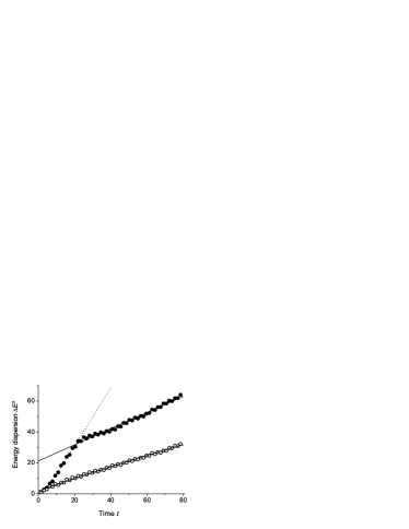
Figure 1: The dependence of the energy dispersion $\Delta E^{2}$ on time $t$ for the natural (filled circles) and randomized (open circles) models. The energy dispersion is measured in the units of $(\hbar\omega_{0})^{2}$. The field strength corresponds to the Fermi point: $F=F_{b}=0.022$; the perturbation frequency $\omega=1.00.$

Figure 1 presents the typical dependence on time of the energy dispersion for the natural (filled circles) and randomized (open circles) models. To extract the value of the energy diffusion coefficient, the numerical dependence was fitted by the law of evolution of the energy dispersion for the diffusion equation with the constant $D$ on the interval $(-L,L)$ with impenetrable walls on the borders and the initial condition in the form of the $\delta(0)$ peak. This dependence can be described (with the local accuracy better than 3%) by the formula

$$\Phi(a,b;t)=a\left({1-\exp\left({-bt}\right)}\right)\times$$ (9)

$$\,\,\,\,\,\,\,\,\left({1+0.633bt\exp\left({-1.161bt}\right)}\right)$$

where $a={{L^{2}}\mathord{\left/{\vphantom{{L^{2}}3}}\right.\kern-1.2pt}3}$ and $b={{6D}\mathord{\left/{\vphantom{{6D}{L^{2}}}}\right.\kern-1.2pt}{L^{2}}}$. The best fits of the formula Eq. (9) with the numerical data are shown in the Fig. 1 by solid lines. The initial moment $t_{0}$ has been used as the third fitting parameter.

For once, it is clearly seen that the randomization suppresses the process of the energy diffusion. Secondly, for the natural model one can see the presence of two different regimes - a fast initial diffusion sharply slows down at a crossover time $t_{c}\simeq 20$. We note that at this moment the energy dispersion $\Delta E^{2}\left({t_{c}}\right)=32\left({\hbar\omega_{0}}\right)^{2}$ is much less than the saturated value $\Delta E_{s}^{2}=a=133\left({\hbar\omega_{0}}\right)^{2}$, that corresponds to the uniform probability distribution throughout the band of the states taken into account. To understand what happens at the crossover time we have to study more closely the time development of the probability distribution.

The overall form of the energy distribution for the natural model is rather accurately approximated by the gaussian form that follows from the model of the energy diffusion with the constant $D$. This agreement can be seen in Fig. 2, where the logarithm of the energy density distribution is shown against the reduced energy shift $\Delta\varepsilon={{\left({E-E_{0}}\right)}\mathord{\left/{\vphantom{{\left({E-E_{0}}\right)}{\hbar\omega_{0}}}}\right.\kern-1.2pt}{\hbar\omega_{0}}}$, where $E_{0}$ is the mean energy value of the initial wavepacket.

Figure 2: The logarithm of the energy density distribution for the time $t=17.3$ for the parameters $F=0.606F_{b},\omega=1.00$. The grassy line is the numerical data, the solid line presents the best fit of data with the parabola $p(\Delta\varepsilon)=\alpha-\beta(\Delta\varepsilon)^{2}$.

Although the agreement seems to be very good, one must keep in mind that the vertical scale of the graph is logarithmic. By subtraction of the parabolic fit from the numerical distribution we come to the picture of deviations that is shown in the Fig. 3.

Figure 3: The deviation of the logarithm of the energy density distribution from the best fitted parabola $\Delta w$ as a function of the dimensionless energy deviation $\Delta\varepsilon$ for the same parameters as in Fig.2. The black stars note the maxima of the ballistic bumps (see the text)

.

The peak at $\Delta\varepsilon=0$ corresponds to the part of the initial packet that is not depleted yet by the energy spreading. Two bumps are clearly seen in the picture: their maxima are located at $\Delta\varepsilon\simeq\pm 12$. The calculations show that these bumps propagate outwards with a constant speed, that is ballistically. The crossover time corresponds to the moment when these bumps reach the borders of the treated band of states. Therefore, only the part of the graph that precedes the $t_{c}$ corresponds to the properties of the model; the second part is just an artifact of the calculation scheme. To estimate the diffusion coefficient we fitted the dependence of the initial state by the two-parameter formula

$$\phi\left({D,\tau;t}\right)=\frac{{2Dt^{2}}}{{\tau+t}},$$ (10)

where the time shift $\tau$ accounts for the duration of the initial stage, where the law of the dispersion growth is always quadratic. The best fitted function $\phi$ is plotted in Fig. 1 by the dashed line.

The ballistic spreading of the energy distribution in the time domain $t>>{{2\pi}\mathord{\left/{\vphantom{{2\pi}\omega}}\right.\kern-1.2pt}\omega}$ is well known for the model of a one-dimensional resonantly excited harmonic oscillator with the Hamiltonian $\hat{H}\left(t\right)={{\left({\hat{p}^{2}+\hat{x}^{2}}\right)}\mathord{\left/{\vphantom{{\left({\hat{p}^{2}+\hat{x}^{2}}\right)}2}}\right.\kern-1.2pt}2}-F\hat{x}\cos t$ . In the quasiclassical domain (for large quantum numbers $n\gg 1$) the matrix elements of the coordinate can be taken constant, $x_{nm}=X\left({\delta_{n,n-1}+\delta_{n,n+1}}\right)$, where $\delta_{ij}$ is the Kroneker delta - symbol. With this assumption in the rotating wave approximation for the initial condition $a_{k}\left(0\right)=\delta_{kn}$ the probabilities $w_{k}$ to find the system in the state $|k>$ are given by the well-known formula

$$w_{k}=|a_{k}(t)|^{2}=J_{n-k}^{2}\left({\Omega t}\right),$$ (11)

where $J_{n}(z)$ are the Bessel functions of the first kind and $\Omega={{FX}\mathord{\left/{\vphantom{{FX}{2\hbar}}}\right.\kern-1.2pt}{2\hbar}}$ is the value of the Rabi frequency. Equation (11) yields for the energy dispersion

$$\Delta E^{2}\left(t\right)=\frac{1}{2}\left({\hbar\omega_{0}\Omega t}\right)^{2}.$$ (12)

However, the randomization of signs of matrix elements does not influence the energy kinetics in this model.

The influence of randomization can be explained by the toy ”double ladder” model. This system has the doubly degenerate equidistant energy spectrum $E_{n}=\hbar\omega_{0}\left[{{n\mathord{\left/{\vphantom{n2}}\right.\kern-1.2pt}2}}\right]$ where $[,]$ denotes the integer part of the number. The matrix elements of the coordinate connect each state $|n>$ to all four states $|m>$ with the energy differences $E_{n}-E_{m}=\pm\hbar\omega_{0}$:

$$x_{nm}=X\left({\delta_{n,n-2}+\delta_{n,n-1}+\delta_{n,n+2}+\delta_{n,n+3}}\right)$$ (13)

for even $n$ and

$$x_{nm}=X\left({\delta_{n,n-3}+\delta_{n,n-2}+\delta_{n,n+1}+\delta_{n,n+2}}\right)$$ (14)

for odd $n$. In this model for the resonant perturbation $\hat{V}\left(t\right)=-F\hat{x}\cos\omega_{0}t$ the energy spreading is ballistic, $\Delta E^{2}\left(t\right)\propto t^{2}$, whereas the randomization of signs leads to the localization of the quasienergy states, and the energy dispersion growth saturates.

One can suppose that the ballistic component in the quantum chaotic model is carried through the subset of states that are similar to the ”double ladder” model. The degree of correlation of the matrix elements can be estimated from the construction

$$T_{n}=\sum\limits_{m,l,k}{x_{nm}x_{ml}x_{lk}x_{kn}},$$ (15)

that describes the sum of contributions of all possible four consequent transitions that start and end on the same state $|n>$. The correlation index $\nu$ can be defined as the ratio of the average value of $T$ for the randomized system to that of the natural system. For the ”double ladder” model we have

$$\nu=\frac{{\left\langle{T_{n}^{R}}\right\rangle}}{{\left\langle{T_{n}^{N}}\right\rangle}}=\frac{7}{{12}}=0.583.$$ (16)

The relatively large value of this number is explained by the large contribution of symmetric contours with $m=k$, that are invariant under the randomization. For the Pullen - Edmonds model the value of the correlation index $\nu=0.72$ is rather close to that of the ”double ladder” model; that makes the analogy plausible.

It must be stressed that the combined effect of the bulk diffusion spreading and the overlaying ballistic bumps propagation produces the linear growth of the energy dispersion (see Fig.1) that will be referred to as the effective diffusion.

We define the repression coefficient $R(F,\omega)$ as the ratio of the effective energy diffusion coefficient to its value $D_{F}$ that follows from the FGR:

$$R\left({F,\omega}\right)=\frac{{D\left({F,\omega}\right)}}{{2\left({\hbar\omega}\right)^{2}\dot{W}_{F}}}.$$ (17)

The dependence of the $R$ on the field strength is shown in Figs. 4 and 5 for two different values of the perturbation frequency.

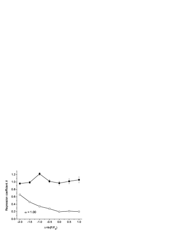
Figure 4: The dependence of the repression coefficient $R$ on the logarithm of the field strength $\Lambda=\ln(F/F_{b})$ for the frequency of perturbation $\omega=1.00$.

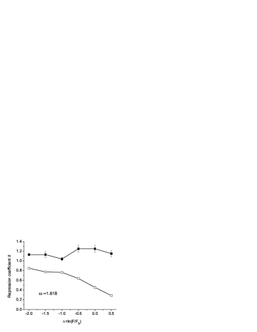
Figure 5: The dependence of the repression coefficient $R$ on the logarithm of the field strength $\Lambda=\ln(F/F_{b})$ for the frequency of perturbation $\omega=1.62$.

For the natural model $R$ remains approximately constant with the value close to unity, whereas for the randomized model the energy diffusion slows down in qualitative agreement with the conclusions of CK00 ; +E06 .

III Energy diffusion in the classical model

The classical expression for the diffusion coefficient Eq. (1) is derived in the limit of the infinitesimal perturbation, when one can neglect the influence of the perturbation on the law of motion of the active coordinate $x(t)$. Let’s study the formation of this coefficient. We represent the external field in the form $F\sin\omega t$ and denote by $t_{n}={{2\pi n}\mathord{\left/{\vphantom{{2\pi n}\omega}}\right.\kern-1.2pt}\omega}$ the moments of time at which the external field take zero values. The variation of the energy for one field period between these moments is exactly proportional to the field strength,

$$\Delta E_{n}=F\int\limits_{t_{n}}^{t_{n+1}}{\dot{x}\left(t\right)}\sin\omega t\,dt=F\Delta_{n}.$$ (18)

The quantities $\Delta_{n}$ we shall call the reduced variations of the energy. In the accepted approximation they do not depend on the field strength.

The following calculations were carried out for the Pullen - Edmonds oscillator on the energy surface $E=11.0$ and for the perturbation frequency $\omega=1.00$.

Figure 6: The dependence of the autocorrelator of the reduced energy increments $B_{\Delta}\left(k\right)=\left\langle{\Delta_{n}\Delta_{n+k}}\right\rangle$ on the time shift $k$ measured in periods of the perturbation on the energy surface $E=11.0$ for the perturbation frequency $\omega=1.00$.

The values of the reduced energy increments $\Delta_{n}$ on the neighbouring time intervals are correlated. Figure 6 presents the form of the autocorrelation function of the reduced energy increments. One can see that for the values of the time shift $k\gtrsim 5$ the correlations become rather small.

The quantity

$$d_{K}=\frac{\omega}{{4\pi K}}\left({\sum\limits_{i=0}^{K-1}{\Delta_{n+i}}}\right)^{2}$$ (19)

will be called the $K$-th approximant of the reduced diffusion coefficient. This is a proportionality coefficient between the diffusion coefficient and the square of the field amplitude, calculated from the interval of time of $K$ consequent periods of the field. The positive correlation of $\Delta_{k}$ for small k produces the initial monotonous growth of the $d_{k}$ that rather rapidly comes to a saturation.

Figure 7: The dependence of the approximants of the reduced diffusion coefficient $d_{n}$ on the duration of the time interval measured in periods of the perturbation for the Pullen - Edmonds model Eq. (6) on the energy surface $E=11.0$ for the perturbation frequency $\omega=1.00$.

From the graph in Fig. (7) it is seen that already $d_{8}$ takes the value that within the 1.5% error margin is undistinguishable from the asymptotic limit. However, this average quantity is formed by the contributions that differ by several orders of magnitude. The graph in Fig. 8 shows the distribution of the quantities $d_{8}$ in the log-log scale. The distribution is taken from averaging over four ensembles of $10^{5}$ points each.

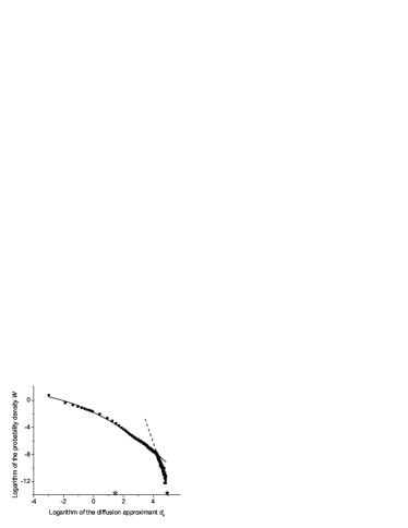
Figure 8: The distribution of the values of partial contributions to the approximant $d_{8}$ from different points on the trajectory of the Pullen - Edmonds model on the energy surface $E=11.0$ for the perturbation frequency $\omega=1.00$. The thin lines show the approximate forms of the distribution given by the formulas in the text. The black star marks the maximal partial contribution $d_{+}$ that comes from the resonant trajectory, the white star marks the position of the average value $<d_{8}>$.

The dominating part of this distribution is accurately fitted by the dependence $\ln w=f(d)=-1.771-1.057\ln d-0.095\left({\ln d}\right)^{2}$ that is shown by the thin solid line. For the largest values of $d_{8}$ another approximation is valid, $\ln w=g(d)=19.268-6.386\ln d$. This dependence is shown in Fig.8 with the thin dashed line. In the domain of validity of the approximation $f(d)$ the slope of the curve is less than unity: the distribution is of the Zipf - Pareto type, in which the dominating contribution to the average comes from the rare large terms. In our case the 20% of the largest terms come with 82% contribution to the average. These large contributions come from the bits of the trajectories in which the point oscillates almost along the direction of the perturbing force nearly synchronously with the perturbation. Theoretically the maximal value of $d_{8}$ originates from the motion with the law $x(t)=\sqrt{2E}\sin(t)$ and equals to $d_{+}=4\pi E/\omega=138.23$.

In this resonant case the energy increment grows linearly in time - that is, ballistically.

Thus we can indicate a classical counterpart to the quantum dynamics of energy growth. The quantum ballistic bumps are analogous to the nearly resonant bits of the classical trajectories with the quasiballistic energy increase.

IV Conclusion

By the numerical studies of the evolution of the energy distribution in a harmonic external field in a system constructed by the quantization of a classically chaotic Hamiltonian system, thus retaining all correlations of the matrix elements, we have found that the effective rate of the energy diffusion preserve its quadratical dependence on the field strength on the domain of the strong field, where the transition rate is comparable to the perturbation frequency. In other words, the Fermi golden rule appears to be valid far beyond the limits of the domain in which its applicability can be justified. This circumstance restores the quantum - classical correspondence for the energy diffusion and the energy absorption rate in the limit $\hbar\to 0$.

We have to admit that our studies are limited to a specific model, studied for two values of the perturbation frequency. However the revealed mechanism of the ballistic component of the energy distribution that propagates through the chains of matrix elements with the correlated signs can be admitted as a universal, especially with the account of the important contribution of the quasiballistic parts of the trajectories to the energy diffusion in the classical model. The more rigorous proof of the universality demands further studies.

References

N. Brenner and Sh. Fishman, Phys. Rev. Lett. 77, 3763 (1996).

P.V. Elyutin and J. Shan, Phys. Rev. Lett. 77, 5043 (1996).

Sh. Mukamel, V. Khidekel, and V. Chernyak, Phys. Rev. E 53, R1 (1996).

D. Cohen, Phys. Rev. Lett. 82, 4951 (1999).

D. Cohen and T. Kottos, Phys. Rev. Lett. 85, 4839 (2000).

A. Iomin, Phys. Rev.E 62, 442 (2000).

K. Morawetz, Phys. Rev. E 61, 2555 (2000).

Ch.H. Reick, Phys. Rev. E 66, 036103 (2002).

P.V. Elyutin, Phys. Rev. E 69, 036207 (2004).

B. Eckhardt, Phys. Reports 163, 205 (1988).

P.V. Elyutin, Usp. Fiz. Nauk 155, 397 (1988) [Sov. Phys. Usp. 31, 597 (1988)].

S. Linkwitz and H. Grabert, Phys. Rev. B-I 44, 11888 (1991).

C. Jarzynski, Phys. Rev. E 48, 4340 (1993).

M. Feingold and A. Peres, Phys. Rev. A 34, 591 (1986).

M. Wilkinson J. Phys. A: Math. Gen. 20, 2415 (1987)

V. Weisskopf and E. Wigner, Zs. Phys. 63, 54 (1930).

L. Allen and J.H. Eberly. Optical Resonance and Two-Level Atoms (NY, John Wiley and Sons, 1975).

N.B. Delone and V.P. Krainov, Usp. Fiz. Nauk 165, 1295 (1995) [Phys. Usp. 38, 1247 (1995)].

P.V. Elyutin, JETP 102, 182 (2006) [ZhETF 129, 207 (2006)].

T. Kottos and D.Cohen, Phys. Rev. E 64, 065202(R) (2001).

R.A. Pullen and A.R. Edmonds, J. Phys. A 14, L477 (1981).

H.-D. Meyer, J. Chem. Phys. 84, 3147 (1986).

P.A. Vorobyev and G.M. Zaslavsky, Sov. Phys. JETP 65, 877 (1987) [ZhETF 92, 1564 (1987)].

P.V. Elyutin and V.G. Korolev, Mosc. Univ. Phys. Bull. 44, 106 (1989) [Vestn. Mosk. Univ. 3 Fiz. Astron. 30, 87 (1989)].