Unmixing in random flows

Abstract

We consider particles suspended in a randomly stirred or turbulent fluid. When effects of the inertia of the particles are significant, an initially uniform scatter of particles can cluster together. We analyse this ‘unmixing’ effect by calculating the Lyapunov exponents for dense particles suspended in such a random three-dimensional flow, concentrating on the limit where the viscous damping rate is small compared to the inverse correlation time of the random flow (that is, the regime of large Stokes number). In this limit Lyapunov exponents are obtained as a power series in a parameter which is a dimensionless measure of the inertia. We report results for the first seven orders. The perturbation series is divergent, but we obtain accurate results from a Padé-Borel summation. We deduce that particles can cluster onto a fractal set and show that its dimension is in satisfactory agreement with previously reported in simulations of turbulent Navier-Stokes flows. We also investigate the rate of formation of caustics in the particle flow.

1 Introduction

1.1 Overview

This paper discusses small particles suspended in a randomly moving fluid. We assume that the fluid flow is mixing, and concentrate on cases where the fluid flow is incompressible (although compressibility is considered too, for completeness). At first sight, it seems as if the particles suspended in an incompressible mixing flow should become evenly distributed. If the particles were simply advected by the fluid, this is indeed what would happen. However, it has been noted that when the effects of finite inertia of the suspended particles are significant, the particles can show a tendency to cluster. This remarkable ‘unmixing’ effect was discussed in a theoretical paper by Maxey [1], who proposed that suspended particles (assumed denser than the fluid) cluster because they are centrifuged away from vortices. There have been many other theoretical papers on this phenomenon, and an experimental demonstration was reported by Eaton and Fessler [2]; the literature is reviewed in section 1.2 below. The suspended particles are characterised by the rate $\gamma$ at which their velocity relative to the fluid is damped due to viscous drag, and the random velocity field is characterised by a correlation time $\tau$. The product $\Omega=\gamma\tau$ is a dimensionless parameter: in much of the literature ${\rm St}=1/\Omega$ is termed the ‘Stokes number’. There is a consensus that the clustering effect is observed when the Stokes number is of order unity.

We investigate a random-flow model with short correlation time, which is susceptible to mathematical analysis. We show that in general this model can exhibit pronounced clustering in circumstances where ${\rm St}\gg 1$, when the centrifuge mechanism is not effective. When the model is applied to fully-developed turbulence it predicts that the clustering is strongest when ${\rm St}=O(1)$ (in agreement with most numerical investigations), but it indicates that the centrifuge effect is not essential to understanding the phenomenon.

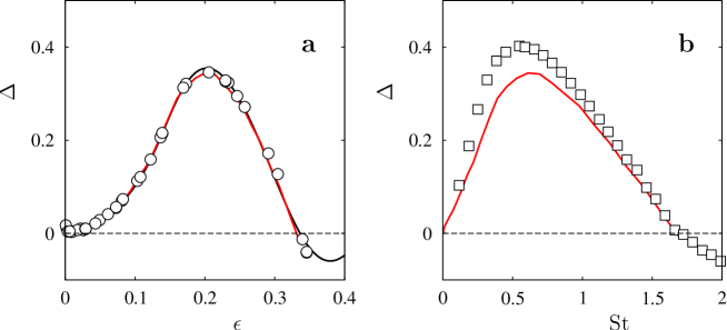
Figure 1: a Dimension deficit $\Delta$ as a function of $\epsilon$, in the limit $\kappa\to 0$; data from simulation of our short-time correlated random-flow model obtained as described in section 3.2 ($\circ$), from a simulation of the Langevin equation (44 - 48), solid red line, and results of a Borel summation of our perturbation series, using a Padé approximant of order $P_{3/3}$ ($-\!\!\!-\!\!\!-\!\!\!-\!\!\!-\!\!\!-$). The figure shows that there is pronounced clustering when $\epsilon=O(1)$: in the limit as $\kappa\to 0$ this happens when ${\rm St}\gg 1$. b Dimension deficit $\Delta$ as a function of Stokes number ${\rm St}$; results (taken from [3]) of direct numerical simulations of particles embedded in Navier-Stokes flows ($\Box$), and results from Langevin equations of our short-time correlated random-flow model, (44 - 48), solid red line. The latter are the same as those in figure 1a, with ${\rm St}=\epsilon^{2}/\kappa^{2}$ and $\kappa=0.256$ was chosen to give a good fit between the curves, as judged by the eye.

Our principal results are series expansions for the Lyapunov exponents of the trajectories of the suspended particles in terms of $\epsilon=\kappa\sqrt{{\rm St}}$, where the dimensionless parameter $\kappa$ (defined in section 1.3 below) is $O(1)$ for fully developed turbulent flow, but may be small for other types of random flow. Our analysis of the random-flow model is exact in the limit as $\kappa\to 0$: note that in this limit ${\rm St}\gg 1$ when $\epsilon=O(1)$. We use the Lyapunov exponents to estimate the ‘dimension deficit’ $\Delta$, which is the difference between the spatial dimension and the (Lyapunov) fractal dimension $d_{\rm L}$ of the set onto which the particles cluster: $d_{\rm L}=3-\Delta$ (this will be explained in section 1.2). Figures 1a and 1b illustrate our results. Figure 1a compares the value of $\Delta$ as a function of $\epsilon$ obtained by simulation of our model with results from a Borel summation of our perturbation series. The results show that there is fractal clustering when $\epsilon=O(1)$ in the limit as $\kappa\to 0$, indicating that fractal clustering can occur for large Stokes numbers. Despite the fact that our perturbation series is divergent, we obtain satisfactory results from Borel summation. Figure 1b compares the results from a direct numerical simulations of particles in a turbulent Navier-Stokes flow (these data ($\Box$) are taken from [3]) with results from our random-flow model: the data used for figure 1a are re-plotted with the value of $\kappa$ chosen to give the best fit between the two curves, as judged by eye. (We cannot determine the scaling theoretically because the value of $\kappa$ for fully developed turbulence is not known). The theoretical curve in figure 1b is obtained from our random-flow model, which has vanishingly small correlation time (because for given $\epsilon$, ${\rm St}\to\infty$ as $\kappa\to 0$). The centrifuge effect cannot therefore cause clustering in this random-flow model. Our model has a maximum dimension deficit of approximately $0.35$, as opposed to $0.40$ for particles in a Navier-Stokes flow, and the form of the curves is similar. We conclude that the random-flow model provides a satisfying degree of agreement with full Navier-Stokes dynamics, despite the fact that the centrifuge mechanism plays no role.

Another mechanism for clustering is the formation of fold caustics in the flow of the particles. We show that caustics are prevalent when $\epsilon>1$. We also consider an explicit expression for the sum of the Lyapunov exponents when the Stokes number is small. Taken together with earlier results on the overdamped limit (referred to in sections 1.2, 8 and 9), our results give a satisfyingly complete understanding of the local dynamics of suspended particles.

Some of the results were summarised in an earlier letter [4].

1.2 Discussion of earlier work

We first briefly review earlier work on clustering in random flows, before giving a fuller description of our results.

Maxey [1] expressed the trajectory of an inertial particle in terms of a ‘synthetic’ velocity field, which is obtained as a perturbation of the velocity field of the fluid. He showed that this synthetic velocity field has negative divergence when the vorticity is high or the strain-rate low, and predicted that particles would have low concentrations in regions of high vorticity due to this ‘centrifuge effect’. A correlation between particle density and vorticity has been seen in direct numerical simulation of particles suspended in a fully-developed turbulent flow [5, 6].

The mechanism proposed by Maxey led to a prediction concerning the observability of this ‘preferential concentration’ effect. It is plausible that the ‘centrifuge mechanism’ will be less effective when the particles are overdamped ($\Omega\gg 1$) or when the velocity fluctuates too rapidly to allow the density of suspended particles to respond (when $\Omega\ll 1$). This leads to the hypothesis that the preferential concentration effect should only be observed when $\Omega$ is close to unity. Experimental work on particles suspended in fully developed turbulent air flows [2] appears to support this hypothesis, as do computer simulations [6, 7, 3].

An alternative approach arises from work of Sommerer and Ott [8], who discuss patterns formed by particles floating on a randomly moving fluid. They characterise these patterns in terms of their fractal dimension, and suggest that the fractal dimension can be obtained from ratios of Lyapunov exponents $\lambda_{i}$ of the particle trajectories, using a formula proposed by Kaplan and Yorke [9]. The argument of Sommerer and Ott extends directly to particles suspended in turbulent three-dimensional flows. The spatial particle flow is characterised by three Lyapunov exponents, $\lambda_{1}>\lambda_{2}>\lambda_{3}$, and provided $\lambda_{1}+\lambda_{2}>0$ (which is always true for the particles moving in an incompressible fluid flow), the Kaplan-Yorke estimate for the fractal dimension is determined by the dimensionless quantity

$$\Delta=-{1\over{|\lambda_{3}|}}(\lambda_{1}+\lambda_{2}+\lambda_{3})$$ (1)

which we term the ‘dimension deficit’. When $\Delta>0$, the Kaplan-Yorke estimate of the dimension, termed the Lyapunov dimension, is

$$d_{\rm L}=3-\Delta$$ (2)

and $d_{\rm L}=3$ if $\Delta\leq 0$. Clustering effects are significant if the fractal dimension is significantly lower than the dimension of space. The relations (1), (2) give a strong motivation to investigate the Lyapunov exponents of suspended particles. Bec [10, 11] has performed detailed numerical investigations for a specific ensemble of random flow fields, showing how the Kaplan-Yorke fractal dimension varies as a function of the Stokes number for his model flow, reaching a minimum for a value of $\Omega$ which is of order unity. These numerical calculations of the dimension deficit are complementary to the ideas proposed by Maxey in [1], in that they quantify the clustering effect without explaining its origin.

The motivation for investigating Lyapunov exponents can also be explained without referring to the fractal dimension. For three-dimensional flows, the sum of the three largest Lyapunov exponents of the particle trajectories may be negative, implying that volume elements almost always contract. However, for incompressible flows the first Lyapunov exponent is always positive, implying that nearby particles almost surely separate. If $(\lambda_{1}+\lambda_{2}+\lambda_{3})/\lambda_{1}$ is negative, there is a tendency for particles to cluster, but if the magnitude of this quantity is small compared to unity the clustering effect will be negligible, because in that case clusters are stretched and folded more rapidly than their density accumulates.

Most of the theoretical work on clustering in turbulent flows has emphasised instantaneous correlations between vortices and particle-density fluctuations. There is an alternative viewpoint on the origin of density fluctuations which is also theoretically tenable, and which is the basis for our own analysis. It can be argued that the density fluctuations are generated by a multiplicative random process: volume elements in the particle flow are randomly compressed or expanded, and the ratio of the final density to the initial density after many multiples of the correlation time $\tau$ can be modeled as a product of a large number of random factors. According to his picture, the density fluctuations will be a record of the history of the flow, and may bear no relation to the instantaneous disposition of vortices when the particle density is measured. The particle density is expected to have a log-normal probability distribution, and the mean value of the logarithm is related to the Lyapunov exponents of the flow. This is another motivation for calculating Lyapunov exponents.

The idea of considering clustering due to random flows has been used in earlier work which adapted results relating to purely advective flows. Most of this literature treats the limiting case where the correlation time of the velocity field is very short, a case which is known as the Kraichnan model [12]. The Lyapunov exponents of such advective flows have been calculated in different ways by several authors: these calculations include results for compressible and solenoidal (incompressible) flows: the earliest calculation appears to be by LeJan [13], who treated a spatially correlated Brownian motion. Later work [14, 15] subsequently showed that the same results apply to a flow with a smooth time dependence, but a very short correlation time. These calculations on purely advective flows cannot explain clustering of particles suspended in incompressible flows, because the density of advected particles remains constant for incompressible flow. Elperin [16] proposed to analyse the motion of inertial particles by applying results derived for advective flows to the synthetic velocity field derived by Maxey [1], which has a compressible component. The same approach was subsequently adopted in [17]. The approximations employed in these papers make use of results from the Kraichnan model of passive scalars [12], valid in the limit where the correlation time $\tau$ approaches zero (St $\rightarrow\infty$). Yet Maxey’s synthetic velocity field is obtained in the overdamped limit where, by contrast, the Stokes number is small, St $\rightarrow 0$.

In summary, the clustering effect can be characterised by calculating the Lyapunov exponents of the particle trajectories, but there is a limited theoretical understanding of these, based on Maxey’s correction to advective flow (which is derived in the limit where $\Omega\ll 1$). There is a consensus that significant clustering only occurs when $\Omega\approx 1$ but there is scope for revising this expectation.

Our own work [18, 19, 20, 21, 4] uses a model for a random flow with a very short correlation time, but the effects of particle inertia are properly accounted for. We remark that a similar approach was proposed by Piterbarg [22], who studied the largest Lyapunov exponent in a two-dimensional flow.

1.3 Plan of paper and summary of results

In section 2, we discuss the dimensionless parameters of the model, and in particular we note the significance of an additional dimensionless parameter, the ‘Kubo number’ (this term is used in the plasma-physics literature, [23]). In terms of a typical fluid velocity $u$ and correlation length $\xi$, the Kubo number is $\kappa=u\tau/\xi$. We argue that $\kappa$ cannot be large, that $\kappa=O(1)$ for fully-developed turbulent flows, and that $\kappa$ may be small in other systems, such as randomly stirred fluids.

Most of our paper is concerned with the case where the Stokes number ${\rm St}=1/\Omega$ is large. This is the underdamped limit where inertial effects are most likely to be significant and where very little work has been done previously. In section 3 we show how the three Lyapunov exponents for inertial particles can be obtained from expectation values of a system of nine coupled stochastic differential equations.

In section 4 we discuss how these general equations can be represented by a system of Langevin equations in the limit where the Stokes number is large and the Kubo number is small. A dimensionless parameter $\epsilon\propto\kappa\,\Omega^{-1/2}$ plays a natural role in these Langevin equations: inertial effects are significant when $\epsilon$ is large.

Section 5 shows how the corresponding Fokker-Planck equation can be mapped to a perturbation of a nine-dimensional isotropic quantum harmonic oscillator. Using the algebra of harmonic-oscillator raising and lowering operators, we develop perturbation expansions for the Lyapunov exponents to large orders in $\epsilon$, with exact expressions for the coefficients. These perturbation expansions are presented in section 6 and are the principal results in this paper.

In the case where inertia is important it is possible for the density to diverge due to the formation of caustics, which are surfaces on which the Jacobian determinant of the particle flow field vanishes. In section 6 we also quantify the rate of formation of these caustic surfaces. Caustics can have a very significant effect on the aggregation of suspended particles, because they can produce a divergent density of particles in a finite time [20] and because they greatly increase the relative velocity of suspended particles [24].

The perturbation series are divergent, and in section 6 we also discuss their summation by Borel-Padé methods. We find excellent agreement with numerical simulations in some cases, but there are revealing discrepancies in other cases: some of our Borel-Padé summations differ from Monte-Carlo evaluations by quantities which have a non-analytic dependence on the perturbation parameter $\epsilon$, of the form $\exp(-\Phi^{\ast}/\epsilon^{2})$ (for some constant $\Phi^{\ast}$). In section 7 we consider a WKB approach to solving the Fokker-Planck equation, and indicate how such non-analytic contributions arise.

Section 8 makes connections between our results and earlier work on Lyapunov exponents of advected particles: we show that the leading-order term in our perturbation series agrees with the Lyapunov exponent for advective flow, and we show that in the limit as $\kappa\to 0$ the same expression for the Lyapunov exponent holds, regardless of whether $\Omega$ is large or small. In the case where the flow is incompressible the sum of the Lyapunov exponents for advected particles is zero. In section 9 we calculate the leading contribution due to the sum of the Lyapunov exponents for particles in an incompressible flow when $\Omega\gg 1$ and $\kappa\ll 1$: the results confirm that $d_{\rm L}$ is very close to $3$ when $\Omega\gg 1$.

Our results have important consequences for the theory of particle clustering. The existing consensus favours the view that clustering only occurs when $\Omega\sim 1$, and is the result of the ‘centrifuge effect’. Our results present a different picture. Clustering onto a fractal set occurs when $\Delta$, defined by (1), is positive, and becomes significant when this number is of order unity. Both simulations and the Borel-Padé summations in section 6 indicate that when $\Omega\ll 1$ and $\kappa\ll 1$, $\Delta$ is positive when $\epsilon$ is less than a critical value $\epsilon_{\rm c}$, and achieves its maximum value of $\Delta_{\rm max}\approx 0.35$ when $\epsilon$ equals $\epsilon_{\rm max}\approx 0.64\epsilon_{\rm c}$. Thus we establish that clustering can be significant when $\Omega\ll 1$, provided that $\kappa\ll 1$. Our results on the overdamped limit obtained in section 9 indicate that although $\Delta>0$ when $\Omega\gg 1$, it is very small, implying that clustering effects are hard to observe when $\Omega\gg 1$. For fully developed turbulence we have $\kappa\sim 1$, which is on the border of the region of validity of our theory, but a plot of $\Delta$ versus ${\rm St}$ for our model (figure 1b) shows satisfying agreement with numerical simulations of turbulent flows (after scaling ${\rm St}$ to account for uncertainties in the definitions of correlations times). This indicates that the centrifuge mechanism makes a marginal contribution to the clustering process. Systems such as randomly stirred fluids, or particles falling under gravity through fully developed turbulence, can exhibit flows where $\kappa\ll 1$, and may exhibit clustering for large values of ${\rm St}$.

2 Formulation of the problem

2.1 Equations of motion

We assume that the particles suspended in the fluid flow satisfy the equations of motion

$$\dot{\mbox{\boldmath$r$}}={1\over{m}}\mbox{\boldmath$p$}\ ,\ \ \dot{\mbox{\boldmath$p$}}=m\gamma\bigl{[}\mbox{\boldmath$u$}(\mbox{\boldmath$r$},t)-\dot{\mbox{\boldmath$r$}}\bigr{]}$$ (3)

where $\mbox{\boldmath$r$}=(r_{1},r_{2},r_{3})$ is the position of a particle, $p$ is the particle momentum, $m$ is its mass and $\mbox{\boldmath$u$}(\mbox{\boldmath$r$},t)$ denotes the velocity field. We neglect effects due to the inertia of the displaced fluid: this is justified when $\rho_{\rm p}/\rho_{\rm f}\gg 1$, where $\rho_{\rm f}$, $\rho_{\rm p}$ are the densities of the fluid and particles respectively. Equations (3) are appropriate for spherical particles when the Reynolds number of the flow referred to the particle diameter is small, and when the particle radius $a$ satisfies $a\ll\xi$. Further conditions are required for the validity of this formula: these can always be satisfied if the radius of the particle and the molecular mean free path of the fluid are sufficiently small [25].

Stokes’s formula gives the relaxation rate

$$\gamma={6\pi a\rho_{\rm f}\nu\over{m}}=\frac{9\rho_{\rm f}\nu}{2\rho_{\rm p}a^{2}}$$ (4)

where $\nu$ is the kinematic viscosity of the fluid. The neglect of the mass of the displaced fluid is an excellent approximation for aerosol systems, and satisfactory for many examples of solid particles in water.

We also assume that the effect of Brownian diffusion of the particles is negligible: the ratio of the particle diffusion constant to the molecular diffusion constant of the fluid is proportional to the ratio of the molecular mean free path to the particle diameter.

2.2 Dimensionless parameters

We characterise the random velocity field by its statistics, denoting the expectation value of a quantity $X$ by $\langle X\rangle$. We assume that the mean velocity is zero: $\langle\mbox{\boldmath$u$}(\mbox{\boldmath$r$},t)\rangle={\bf 0}$. The velocity field can be characterised by its correlation function, which has a correlation length $\xi$ and a correlation time $\tau$. The fluctuations of the fluid velocity have a characteristic scale $u$: in a single-scale flow we would define $u^{2}=\langle\mbox{\boldmath$u$}^{2}\rangle$, but in fully developed turbulence it is more natural to define $u$ as the velocity scale associated with fluctuations on the dissipative scale, $u=({\cal E}\nu)^{1/4}$, where ${\cal E}$ is the rate of dissipation per unit mass [26].

The equations of motion (3) are characterised by four dimensional parameters. The random velocity field is described by three scales: $u$, $\xi$ and $\tau$. In addition, the interaction of the fluid with the particles is described by the damping rate $\gamma$. (The mass $m$ can be eliminated from the two components of (3), but may appear in expressions which contain forces). From the four quantities $\xi,\tau,u,\gamma$ we can form two independent dimensionless groups, the Kubo number, $\kappa$ and the Stokes number, $1/\Omega$. The degree to which the velocity field is compressible is described by a further dimensionless variable, $\Gamma$, which will be defined in section 4. The average number of suspended particles per unit volume, $N_{0}$, is associated with a further independent dimensionless parameter, $\Upsilon=N_{0}\xi^{3}$. The set of dimensionless parameters of the system is therefore

$$\kappa={u\tau\over{\xi}}\ ,\ \ \ \Omega=\gamma\tau\ ,\ \ \ \Gamma\ ,\ \ \ \Upsilon=N_{0}\xi^{3}\,.$$ (5)

We consider flow fields ranging from incompressible flow (which corresponds to $\Gamma=2$, see equation (43) in section 4) to pure potential flow ($\Gamma={1\over 3}$). We concentrate on the underdamped limit ($\Omega\ll 1$, large Stokes number), but also give results for the overdamped situation.

We argue on physical grounds that $\kappa$ cannot be large, and that $\kappa\sim 1$ for fully developed turbulence. For real flows satisfying the Navier-Stokes equations, the velocity field is self-convected, so that temporal variations of the velocity field at any point are partly due to the ‘sweeping’ action of the flow. If $u$ is the characteristic velocity and $\xi$, $\tau$ are the spatial and temporal correlation scales, then the transport of the velocity field by its own action will cause it to fluctuate on a time scale $\xi/u$, which cannot be less than the actual correlation time of the field. Thus $\kappa=u\tau/\xi$ cannot be large. Small Kubo numbers are realised in randomly stirred fluids where the Reynolds number is small enough that the flow does not spontaneously generate turbulence. For fully developed turbulence, the Kolmogorov theory [26] indicates that $u$, $\xi$ and $\tau$ are all functions of ${\cal E}$ and $\nu$, and dimensional considerations imply that $\kappa\sim 1$. Our analytical results are all derived in the limit where $\kappa\ll 1$, so that fully-developed turbulence is on the borderline of applicability of our theory.

A practically important measure of the degree of clustering is given by the ratio of the largest observed particle density $N_{\rm max}$ to the mean particle density. The parameter $\Upsilon$ will have a pronounced effect on the distribution pattern of the particles. When $\Upsilon$ is sufficiently small, the particles will appear as a random scatter if the largest Lyapunov exponent (defined below) is positive. The set of particle positions is a point set which randomly samples a fractal measure, but the fractal is only visible when $\Upsilon$ is sufficiently large. For large $\Upsilon$, the density-enhancement factor $N_{\rm max}/N_{0}$ may be very large, even when the parameter $\Delta$ (defined by (1)) is small. A quantitative discussion of these issues would be quite lengthy. Accordingly, in this paper we will consider only locally defined properties of the particle trajectories, namely the Lyapunov exponents and the rate of caustic formation, both of which are defined below.

We remark that the dimensionless parameters $\kappa$ and $\Upsilon$ have apparently not been considered in earlier papers on clustering of particles in random flow fields. Uncertainties about the intended values of these parameters makes some of the literature quite difficult to understand.

2.3 Definitions of rate constants

The Lyapunov exponents $\lambda_{i}$, $i=1,2,3$ are rate constants which are defined in terms of the time dependence of small separations of trajectories from a reference trajectory $\mbox{\boldmath$r$}(t)$. We consider three trajectories which have infinitesimal displacements from the reference trajectory, $\delta\mbox{\boldmath$r$}_{i}(t)$, $i=1,2,3$. We then consider the length $\delta r=|\delta\mbox{\boldmath$r$}_{1}|$ of a small separation between two trajectories, the area $\delta{\cal A}=|\mbox{\boldmath$r$}_{1}\wedge\mbox{\boldmath$r$}_{2}|$ of a parallelogram spanned by two separation vectors and the volume $\delta{\cal V}=|\mbox{\boldmath$r$}_{3}\cdot\mbox{\boldmath$r$}_{2}\wedge\mbox{\boldmath$r$}_{3}|$ of a parallelepiped spanned by a triad of separations. The Lyapunov exponents are defined by writing

$$\lambda_{1} = \lim_{t\to\infty}{1\over t}\log_{\rm e}(\delta r)$$

$$\lambda_{1}+\lambda_{2} = \lim_{t\to\infty}{1\over t}\log_{\rm e}(\delta{\cal A})$$

$$\lambda_{1}+\lambda_{2}+\lambda_{3} = \lim_{t\to\infty}{1\over t}\log_{\rm e}(\delta{\cal V})\ .$$ (6)

If $\lambda_{1}<0$, pairs of particles coalesce with probability unity. If $\lambda_{1}>0$ and $\lambda_{1}+\lambda_{2}<0$, particles cluster onto randomly moving lines, which stretch and fold. If $\lambda_{1}+\lambda_{2}>0$ but $\lambda_{1}+\lambda_{2}+\lambda_{3}<0$, the particles cluster onto randomly stretching and folding surfaces.

2.4 Caustics

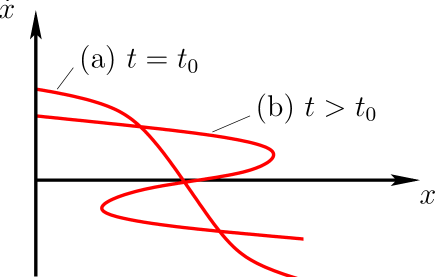
Figure 2: Schematic illustration of a caustic in one spatial dimension: the velocity $\dot{x}$ of the particles as a function of position $x$ is initially single-valued (curve (a)) but particles with a large velocity overtake slower-moving particles, so that at a later time the particle velocity is multi-valued (curve (b)). The region where the velocity is a multi-valued function is bounded by two fold caustics.

Another locally defined statistic is the rate of caustic formation. There is no constraint which prevents two of the three vectors defining the separation between nearby particles becoming collinear, so that the volume element $\delta{\cal V}$ becomes zero for an instant in time. These events correspond to ‘caustics’, where faster moving particles overtake slower ones [27, 20, 24] (see figure 2 for an illustration in one spatial dimension). Caustics influence the spatial particle distribution and the relative velocities of nearby particles.

There is an increased density of particles on the fold caustics (which are a pair of points in the one-dimensional example of figure 2, but which form surfaces in three dimensions), and the particle density on the caustics diverges in the limit as $\Upsilon\to\infty$. This effect is discussed in [27, 20]: it is analogous to the divergence of light intensity on optical caustics [28].

The other effect of caustics is that the particle velocity field becomes multi-valued in the region between the caustics (in figure 2 the velocity field is triple-valued between the caustics). Because particles at the same position are moving with differing velocities, the caustics enhance the rate of collision of suspended particles [27, 20] (this has no analogue in optical caustics). Caustics therefore facilitate the aggregation of suspended particles.

We define $J$, the rate of caustic formation, as the rate at which events where $\delta{\cal V}=0$ occur for a given triplet of nearby trajectories. We define a dimensionless rate $J^{\prime}$ by $J^{\prime}=J/\gamma$.

3 Equations determining the Lyapunov exponents

3.1 Stochastic differential equations for the Lyapunov exponents

Linearising the equations of motion (3) gives

$$\delta\dot{\mbox{\boldmath$p$}} = -\gamma\delta\mbox{\boldmath$p$}+{\bf F}(t)\delta\mbox{\boldmath$r$}$$

$$\delta\dot{\mbox{\boldmath$r$}} = {1\over m}\delta\mbox{\boldmath$p$}\ .$$ (7)

where ${\bf F}(t)$ is a matrix with elements proportional to the rate-of-strain matrix:

$$F_{\mu\nu}(t)=\gamma m\,{\partial u_{\mu}\over{\partial r_{\nu}}}(\mbox{\boldmath$r$}(t),t)$$ (8)

(from this point we will use Greek subscripts to label components in three dimensional space, reserving Roman indices for components in a nine-dimensional space which appears later). To determine the Lyapunov exponents we consider three trajectories displaced relative to a reference trajectory by $(\delta\mbox{\boldmath$r$}_{\mu},\delta\mbox{\boldmath$p$}_{\mu})$, with $\mu=1,2,3$. We choose to parametrise the spatial displacements as follows

$$\delta\mbox{\boldmath$r$}_{1} = X_{1}{\bf n}_{1}$$

$$\delta\mbox{\boldmath$r$}_{2} = X_{2}({\bf n}_{1}+\delta\theta{\bf n}_{2})$$

$$\delta\mbox{\boldmath$r$}_{3} = X_{3}[{\bf n_{1}}+\delta\theta\delta\phi(Z{\bf n}_{2}+{\bf n}_{3})]$$ (9)

where the ${\bf n}_{\mu}(t)$ form a triplet of orthogonal unit unit vectors. Nine variables are required to parametrise the spatial displacements $\delta\mbox{\boldmath$r$}_{\mu}$. Two parameters specify the direction of ${\bf n}_{1}$, and a further angular parameter specifies the direction of ${\bf n}_{2}$ relative to ${\bf n}_{1}$. There is only a binary choice in the direction of ${\bf n}_{3}$, and we resolve this by requiring continuity. This means that a further six parameters are required, and (3.1) does indeed contain a further six parameters, namely $(X_{1},X_{2},X_{3},Z,\delta\theta,\delta\phi)$.

For the choice of parametrisation above, the small elements required in (2.3) are $\delta r=X_{1}$, $\delta{\cal A}=X_{1}X_{2}\delta\theta$ and $\delta{\cal V}=X_{1}X_{2}X_{3}\delta\theta^{2}\delta\phi$. We can then extract the Lyapunov exponents from expectation values of logarithmic derivatives of the variables used in our parametrisation:

$$\lambda_{1} = \biggl{\langle}{\dot{X}_{1}\over{X_{1}}}\biggr{\rangle}$$

$$\lambda_{2} = \biggl{\langle}{\dot{X}_{2}\over{X_{2}}}\biggr{\rangle}+\biggl{\langle}{\delta\dot{\theta}\over{\delta\theta}}\biggr{\rangle}$$

$$\lambda_{3} = \biggl{\langle}{\dot{X}_{3}\over{X_{3}}}\biggr{\rangle}+\biggl{\langle}{\delta\dot{\phi}\over{\delta\phi}}\biggr{\rangle}+\biggl{\langle}{\delta\dot{\theta}\over{\delta\theta}}\biggr{\rangle}\ .$$ (10)

The angles $\delta\theta$ and $\delta\phi$ both decrease with probability unity, and eventually we retain only leading orders in these variables. Initially, however, we retain all terms.

The equations of motion for the displacements $\delta\mbox{\boldmath$r$}_{\mu}$ also contain corresponding increments of momentum, $\delta\mbox{\boldmath$p$}_{\mu}$. These will be parametrised in terms of the nine elements of a $3\times 3$ matrix $\bf R$ by writing

$$\delta\mbox{\boldmath$p$}_{\mu}={\bf R}\,\delta\mbox{\boldmath$r$}_{\mu}\ .$$ (11)

Substituting this relation into (3.1) gives the equation of motion for $\bf R$:

$${{\rm d}{\bf R}\over{{\rm d}t}}=-\gamma{\bf R}-{1\over m}{\bf R}^{2}+{\bf F}(t)\ .$$ (12)

Now we determine the equations of motion for the parameters determining $\delta\mbox{\boldmath$r$}$. Differentiating each line of (3.1) with respect to time, and then using the second equation of (3.1), we obtain

$$\dot{X}_{1}{\bf n}_{1}+X_{1}\dot{\bf n}_{1}$$

$$\hskip 28.45274pt={1\over m}X_{1}{\bf R}(t){\bf n}_{1}$$

$$\dot{X}_{2}({\bf n}_{1}+\delta\theta{\bf n}_{2})+X_{2}(\dot{\bf n}_{1}+\delta\theta\dot{\bf n}_{2})+X_{2}\delta\dot{\theta}{\bf n}_{2}$$

$$\hskip 28.45274pt={1\over m}X_{2}{\bf R}(t)({\bf n}_{1}+\delta\theta{\bf n}_{2})$$

$$\dot{X}_{3}[{\bf n}_{1}+\delta\theta\delta\phi(Z{\bf n}_{2}+{\bf n}_{3})]+X_{3}[\dot{\bf n}_{1}+\delta\theta\delta\phi(Z\dot{\bf n}_{2}+\dot{\bf n}_{3})]$$

$$\hskip 28.45274pt+X_{3}(\delta\dot{\theta}\delta\phi+\delta\theta\delta\dot{\phi})(Z{\bf n_{2}}+{\bf n}_{3})+X_{3}\delta\theta\delta\phi\dot{Z}{\bf n}_{2}$$

$$\hskip 28.45274pt={1\over m}X_{3}{\bf R}(t)[{\bf n}_{1}+\delta\theta\delta\phi(Z{\bf n}_{2}+{\bf n}_{3})]\ .$$ (13)

We now take the scalar product of each of these three equations with each of the unit vectors ${\bf n}_{\mu}$ in turn. It is convenient to use the notations

$$R^{\prime}_{\mu\nu}(t)={\bf n}_{\mu}(t)\cdot{\bf R}(t)\,{\bf n}_{\nu}(t)\ ,\ \ \ F^{\prime}_{\mu\nu}(t)={\bf n}_{\mu}(t)\cdot{\bf F}(t)\,{\bf n}_{\nu}(t)$$ (14)

for the elements of the tensors ${\bf F}$ and ${\bf R}$ transformed to the rotated basis. Taking the scalar product of the first equation of (3.1) with each of the unit vectors leads to the equations

$${\dot{X}_{1}\over{X_{1}}}={1\over m}R^{\prime}_{11}(t)$$ (15)

$$\dot{\bf n}_{1}\cdot{\bf n}_{2}={1\over m}R^{\prime}_{21}(t)$$ (16)

$$\dot{\bf n}_{1}\cdot{\bf n}_{3}={1\over m}R^{\prime}_{31}(t)\ .$$ (17)

Now taking the scalar product of the second equation of (3.1) with each unit vector in turn, and using (15) to (17) to simplify gives, respectively

$${\dot{X}_{2}\over{X_{2}}}={\dot{X}_{1}\over{X_{1}}}+{1\over m}\delta\theta[R^{\prime}_{12}(t)+R^{\prime}_{21}(t)]$$ (18)

$${\delta\dot{\theta}\over{\delta\theta}}={1\over m}[R^{\prime}_{22}(t)-R^{\prime}_{11}(t)]-{\delta\theta\over{m}}[R^{\prime}_{12}(t)+R^{\prime}_{21}(t)]$$ (19)

$$\dot{\bf n}_{2}\cdot{\bf n}_{3}={1\over m}R^{\prime}_{32}(t)\,.$$ (20)

Using the final equation of (3.1), and making use of (15) to (20) to simplify, we find

$${\dot{X}_{3}\over{X_{3}}}={\dot{X}_{1}\over{X_{1}}}+{1\over m}\delta\theta\delta\phi\biggl{(}Z[R^{\prime}_{12}(t)+R^{\prime}_{21}(t)]+R^{\prime}_{13}(t)+R^{\prime}_{31}(t)\biggr{)}$$ (21)

$${\delta\dot{\phi}\over{\delta\phi}}={1\over m}[R^{\prime}_{33}(t)-R^{\prime}_{22}(t)]+{\delta\theta\over{m}}[R^{\prime}_{12}(t)+R^{\prime}_{21}(t)]-{\delta\theta\delta\phi\over{m}}\biggl{(}Z[R^{\prime}_{12}(t)+R^{\prime}_{21}(t)]+R^{\prime}_{13}(t)+R^{\prime}_{31}(t)\biggr{)}$$ (22)

$$\dot{Z}={1\over m}[R^{\prime}_{23}(t)+R^{\prime}_{32}(t)]+{1\over m}Z[R^{\prime}_{22}(t)-R^{\prime}_{33}(t)]\,.$$ (23)

Equations (15) to (23) are the exact equations of motion for the nine variables parametrising $\delta\mbox{\boldmath$r$}$. Retaining only the leading-order terms in $\delta\theta$ and $\delta\phi$, we have

$${\dot{X}_{1}\over X_{1}}={1\over m}R^{\prime}_{11}\ ,\ \ \ {\delta\dot{\theta}\over{\delta\theta}}={1\over m}(R^{\prime}_{22}-R^{\prime}_{11})\ ,\ \ \ {\delta\dot{\phi}\over{\delta\phi}}={1\over m}(R^{\prime}_{33}-R^{\prime}_{22})\,.$$ (24)

Using equation (3.1), we find the following expressions for the Lyapunov exponents:

$$\lambda_{1}={1\over m}\langle R^{\prime}_{11}\rangle\ ,\ \ \ \lambda_{2}={1\over m}\langle R^{\prime}_{22}\rangle\ ,\ \ \ \lambda_{3}={1\over m}\langle R^{\prime}_{33}\rangle\ .$$ (25)

The Lyapunov exponents are thus obtained directly from the elements of $\langle{\bf R}^{\prime}\rangle$ which satisfies an equation similar to (12): to derive it, write ${\bf n}_{\mu}={\bf O}\,{\bf e}_{\mu}$ where ${\bf e}_{\mu}$ are the unit vectors of a fixed Cartesian coordinate system, ${\bf n}_{\mu}$ were introduced in (3.1), and ${\bf O}$ is an orthogonal matrix. Transforming (12)

$${\bf O}^{+}\dot{\bf R}{\bf O}=-\gamma{\bf R}^{\prime}-\frac{1}{m}{{\bf R}^{\prime}}^{2}+{\bf F}^{\prime}\,.$$ (26)

Making use of

$${\bf O}^{+}\dot{\bf R}{\bf O}=\dot{{\bf R}^{\prime}}-[{\bf R}^{\prime},{\bf O}^{+}\dot{\bf O}]$$ (27)

we obtain

$$\dot{{\bf R}^{\prime}}=-\gamma{\bf R}^{\prime}-\frac{1}{m}{{\bf R}^{\prime}}^{2}+[{\bf R}^{\prime},{\bf O}^{+}\dot{\bf O}]+{\bf F}^{\prime}\,.$$ (28)

The matrix elements of ${\bf O}^{+}\dot{\bf O}$ are given by (16), (17), and (20)

$${\bf O}^{+}\dot{\bf O}=\frac{1}{m}\left(\begin{array}[]{lcr}0&-R_{21}^{\prime}&-R_{31}^{\prime}\\ R_{21}^{\prime}&0&-R_{32}^{\prime}\\ R_{31}^{\prime}&R_{32}^{\prime}&0\end{array}\right)\,.$$ (29)

To summarise: the Lyapunov exponents are determined by (25), using expectation values of variables occurring in the system of stochastic differential equations defined by (28) and (29).

3.2 Numerical calculation of Lyapunov exponents

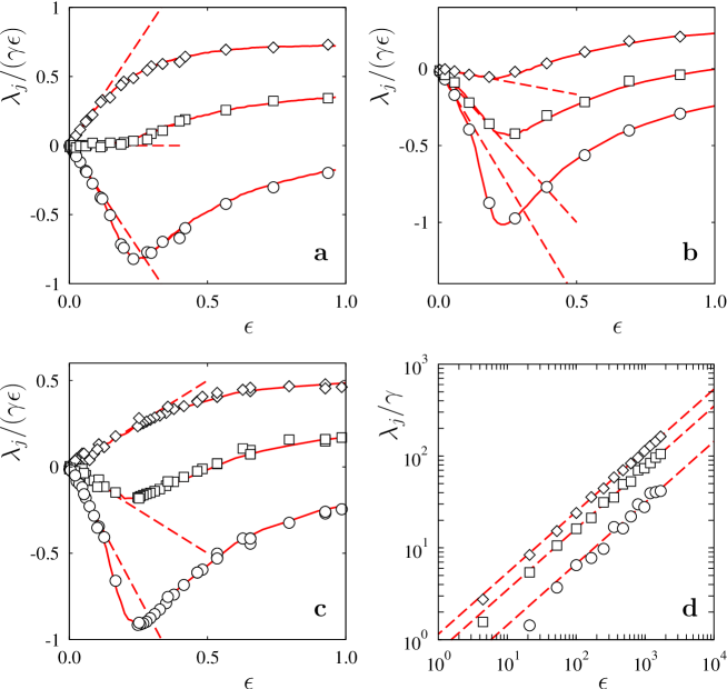
Figure 3: Lyapunov exponents $\lambda_{j}$ as a function of $\epsilon$ for $j=1,2,3$ and three different values of $\Gamma$. Panels a - c show numerical simulations using a discretised form of the equations of motion (3), replacing the force field by a random variable with appropriate statistics as described in section 3.2: $\diamond$ ($j=1$), $\Box$ ($j=2$), and $\circ$ ($j=3$). Also shown are results of Monte-Carlo simulation of the Langevin equation (44), solid lines, as well as the lowest-order estimates (94), dashed lines. Panel a: $\Gamma=2$ (incompressible flow). Panel b: $\Gamma=1/3$ (pure potential flow). Panel c: $\Gamma=1$. Panel d shows large-$\epsilon$ behaviour of the numerical data from a, also shown are fits to the large-$\epsilon$ behaviour (49), dashed lines.

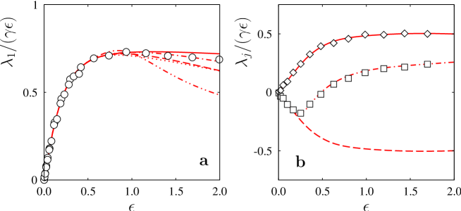
Figure 5: Borel-Padé summation of the perturbation expansion of $\lambda_{j}$. a: Numerical data for $\lambda_{1}$ as a function of $\epsilon$ for $\Gamma=2$ ($\circ$) (obtained as described in section 3.2), compared with results of Borel-Padé summation, equations (92) and (93); $P_{5/5}$ ($---$), $P_{10/10}$ ($-\cdot-\cdot-$), $P_{15/15}$ ($-\cdot\cdot-\cdot\cdot-$), and $P_{20/20}$ ($\cdot\cdot\cdot\cdot\cdot\cdot\cdot$). and $P_{23/23}$ ($-\!\!\!-\!\!\!-\!\!\!-\!\!\!-\!\!\!-$). b: Numerical data for $\lambda_{1}$ ($\diamond$) and $\lambda_{2}$ ($\Box$) as a function of $\epsilon$ for $\Gamma=1$. Also shown are results of Padé-Borel summation (using a Padé approximant $P_{23/23}$) for $j=1$ (solid line) and $j=2$ (dashed line). Since according to equation (6.3) $c_{l}^{(2)}=-c_{l}^{(1)}$ at $\Gamma=1$, those curves are identical apart from an overall minus sign. But using the relation $\lambda_{1}+\lambda_{2}\sim C\exp[-1/(6\,\epsilon^{2})]$, with $\lambda_{1}$ obtained by Borel-Padé summation and $C=0.79$ a fitted parameter ($-\cdot-\cdot-$) gives a much better fit to $\lambda_{2}$ than the dashed line.

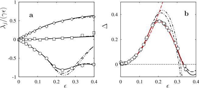
Figure 6: a dependence of the Lyapunov exponents on $\epsilon$, for $\Gamma=2$: the symbols show numerical data obtained as described in section 3.2, and the solid lines are the results of Borel-Padé summation. The results for $\lambda_{3}$ depend upon the number of orders of the perturbation series included in the Borel sum, $P_{2/2}$ ($-\cdot\cdot-\cdot\cdot-$), $P_{2/3}$ ($-\cdot-\cdot-$), $P_{3/3}$ ($---$), and $P_{3/4}$ ($-\!\!\!-\!\!\!-\!\!\!-\!\!\!-\!\!\!-$). b dimension deficit obtained from the curves in figure 6a using equation (1): the same line styles are used for different Padé approximants. The solid red curve shows the results of Monte-Carlo simulations of the Langevin equation (44 - 48), and is the same as in figure 1a. The dashed red line is the asymptotic approximation (95).

Our numerical results for the Lyapunov exponents, represented as symbols in figures 1, 3, 5, and 6, were obtained in the limit of $\tau\rightarrow 0$ by discretising time in equation (3.1). We write $t=n\delta t$ with $n=0,1,2,\ldots$, and with a time step $\delta t$ which satisfies $1/\gamma\gg\delta t\gg\tau$. Writing $\delta\mbox{\boldmath$r$}_{n}=\delta\mbox{\boldmath$r$}(n\delta t)$ and $\delta\mbox{\boldmath$p$}_{n}=\delta\mbox{\boldmath$p$}(n\delta t)$ the Euler discretisation of (3.1) is

$$\left(\begin{array}[]{c}\delta\mbox{\boldmath$r$}^{(n+1)}\\ \delta\mbox{\boldmath$p$}^{(n+1)}\end{array}\right)=\left(\begin{array}[]{ll}{\bf I}&{\bf I}\,(\delta t/m)\\ {\bf F}^{(n)}\delta t&{\bf I}\,(1-\gamma\delta t)\end{array}\right)\left(\begin{array}[]{c}\delta\mbox{\boldmath$r$}^{(n)}\\ \delta\mbox{\boldmath$p$}^{(n)}\end{array}\right)\equiv{\bf M}^{(n)}\left(\begin{array}[]{c}\delta\mbox{\boldmath$r$}^{(n)}\\ \delta\mbox{\boldmath$p$}^{(n)}\end{array}\right)\,.$$ (30)

Here ${\bf F}^{(n)}$ is a matrix with elements

$$F_{\mu\nu}^{(n)}=m\gamma\int_{n\delta t}^{(n\!+\!1)\delta t}\!\!{\rm d}t^{\prime}\,\,\frac{\partial u_{\mu}(\mbox{\boldmath$r$}_{t^{\prime}},t^{\prime})}{\partial r_{\nu}}$$ (31)

with $\mu,\nu=1,2,3$, and ${\bf I}$ is the $3\times 3$ unit matrix. The random components $F_{\mu\nu}^{(n)}$ average to zero, are uncorrelated for $n\neq n^{\prime}$, and the correlation $\langle F_{\mu\nu}^{(n)}F_{\mu^{\prime}\nu^{\prime}}^{(n)}\rangle$ is determined by the statistical properties of $\mbox{\boldmath$u$}(\mbox{\boldmath$r$},t)$ described in section 4.1. The Lyapunov exponents are identified as the asymptotic growth rates of the three largest eigenvalues of the product ${\bf M}^{(N)}{\bf M}^{(N-1)}\cdots{\bf M}^{(0)}$ nearly diagonal matrices for large values of $N$. The asymptotic growth rates are determined using a method described in [29].

4 Langevin equations for Lyapunov exponents

4.1 Equations in Langevin form

The equation (28) for ${\bf R}^{\prime}$ can be simplified when the correlation time of the velocity field is sufficiently short, and when the amplitude of the random force is sufficiently small. In this limit the force-gradient term ${\bf F}^{\prime}$ behaves like a white-noise signal, and the equations of motion reduce to a system of Langevin equations:

$${\rm d}{\bf R}^{\prime}=\biggl{(}-\gamma{\bf R}^{\prime}-\frac{1}{m}{{\bf R}^{\prime}}^{2}+[{\bf R}^{\prime},{\bf O}^{+}\dot{\bf O}]\biggr{)}{\rm d}t+{\rm d}\mbox{\boldmath$\zeta$}$$ (32)

where ${\rm d}\mbox{\boldmath$\zeta$}$ is a matrix of random increments ${\rm d}\zeta_{\mu\nu}$ satisfying

$$\langle{\rm d}\zeta_{\mu\nu}\rangle=0\ ,\ \ \ \langle{\rm d}\zeta_{\mu\nu}{\rm d}\zeta_{\mu^{\prime}\nu^{\prime}}\rangle=2{\cal D}_{\mu\nu,\mu^{\prime}\nu^{\prime}}{\rm d}t\ .$$ (33)

The elements ${\cal D}_{\mu\nu,\mu^{\prime}\nu^{\prime}}$ of the ‘diffusion matrix’ depend on the statistics of the fluid velocity field $\mbox{\boldmath$u$}(\mbox{\boldmath$r$},t)$. The latter may be decomposed into potential and solenoidal components, generated from scalar and vector potentials. The Stokes drag force on the particle, $\mbox{\boldmath$f$}=m\gamma\mbox{\boldmath$u$}$ is written in terms of potentials $\phi$ and $A$:

$$\mbox{\boldmath$f$}=\mbox{\boldmath$\nabla$}\phi+\mbox{\boldmath$\nabla$}\wedge\mbox{\boldmath$A$}\ .$$ (34)

The fields $\phi(\mbox{\boldmath$r$},t)\equiv A_{0}(\mbox{\boldmath$r$},t)$ and $A_{\mu}(\mbox{\boldmath$r$},t),\,\mu=1,2,3$ are assumed to possess statistical properties which are homogeneous in space and time, and isotropic in space. Also, it is assumed that these fields are uncorrelated, and the intensity of the $A_{\mu}$ fields (for $\mu=1,2,3$) is such that the correlation function is of the form

$$\langle A_{\mu}(\mbox{\boldmath$r$}_{0}+\mbox{\boldmath$R$},t_{0}+t)A_{\nu}(\mbox{\boldmath$r$}_{0},t_{0})\rangle=\delta_{\mu\nu}[(1-\alpha^{2})\delta_{\mu 0}+\alpha^{2}]\,C(R,t)$$ (35)

for some constant $\alpha$, where $R=|\mbox{\boldmath$R$}|$.

Using spatial and temporal homogeneity of the velocity field, and noting that in the limit ${\rm Ku}\to 0$ the particle does not move significantly in time $\tau$, elements of the diffusion matrix are

$${\cal D}_{\mu\nu,\mu^{\prime}\nu^{\prime}}={\textstyle{1\over 2}}\int_{-\infty}^{\infty}{\rm d}t\ \biggl{\langle}{\partial f_{\mu}\over{\partial r_{\nu}}}({\mbox{\boldmath$0$}},t){\partial f_{\mu^{\prime}}\over{\partial r_{\nu^{\prime}}}}(\mbox{\boldmath$0$},0)\biggr{\rangle}\ .$$ (36)

Inserting the expression (34) for the force gives an expression for these elements in terms of second derivatives of the fields $A_{\mu}$. For any isotropic field $A(\mbox{\boldmath$r$},t)$, these satisfy, for example,

$$\biggl{\langle}{\partial^{2}A\over{\partial r_{1}^{2}}}(\mbox{\boldmath$r$},t){\partial^{2}A\over{\partial r_{1}^{2}}}(\mbox{\boldmath$r$},0)\biggl{\rangle}=3\biggl{\langle}{\partial^{2}A\over{\partial r_{1}\partial r_{2}}}(\mbox{\boldmath$r$},t){\partial^{2}A\over{\partial r_{1}\partial r_{2}}}(\mbox{\boldmath$r$},0)\biggl{\rangle}=3\biggl{\langle}{\partial^{2}A\over{\partial r_{1}^{2}}}(\mbox{\boldmath$r$},t){\partial^{2}A\over{\partial r_{2}^{2}}}(\mbox{\boldmath$r$},0)\biggl{\rangle}\ .$$ (37)

Now consider the evaluation of the elements of the diffusion matrix, ${\cal D}_{\mu\nu,\mu^{\prime}\nu^{\prime}}$. First we note that due to isotropy, the values of the elements are invariant under any permutation of indices (for example, ${\cal D}_{33,22}={\cal D}_{11,33}$). It is easy to see that ${\cal D}_{\mu\nu,\mu^{\prime}\nu^{\prime}}=0$ unless the four indices can be grouped into two equal pairs. There are four cases where indices are paired, namely ${\cal D}_{aa,bb}$, ${\cal D}_{ab,ab}$, ${\cal D}_{ab,ba}$ and ${\cal D}_{aa,aa}$ where $a$ and $b$ are different numbers from the set $\{1,2,3\}$. We define

$${\cal D}_{0}={\textstyle{1\over 2}}\int_{-\infty}^{\infty}{\rm d}t\ \biggl{\langle}{\partial^{2}\phi\over{\partial r_{1}^{2}}}({\bf 0},t){\partial^{2}\phi\over{\partial r_{1}^{2}}}({\bf 0},0)\biggr{\rangle}$$ (38)

and use (37) to express the non-zero elements ${\cal D}_{\mu\nu,\mu^{\prime}\nu^{\prime}}$ in terms of ${\cal D}_{0}$ and $\alpha^{2}$. It is simplest to calculate specific examples of the non-zero elements, and to deduce the others by permuting indices: writing $\partial^{2}A_{\mu}/\partial r_{\nu}\partial r_{\rho}(\mbox{\boldmath$r$},t)$ in shorthand as $(\partial^{2}_{\nu\rho}A_{\mu})_{t}$, we have

$${\cal D}_{11,11} = {\textstyle{1\over 2}}\int_{-\infty}^{\infty}{\rm d}t\ \langle(\partial^{2}_{11}\phi+\partial^{2}_{21}A_{3}-\partial^{2}_{31}A_{2})_{t}(\partial^{2}_{11}\phi+\partial^{2}_{21}A_{3}-\partial^{2}_{31}A_{2})_{0}\rangle$$

$$= {\cal D}_{0}\biggl{(}1+{2\alpha^{2}\over 3}\biggr{)}\equiv{\cal D}_{1}$$

$${\cal D}_{12,12} = {\textstyle{1\over 2}}\int_{-\infty}^{\infty}{\rm d}t\ \langle(\partial^{2}_{12}\phi+\partial^{2}_{22}A_{3}-\partial^{2}_{32}A_{2})_{t}(\partial^{2}_{12}\phi+\partial^{2}_{22}A_{3}-\partial^{2}_{32}A_{2})_{0}\rangle$$

$$= {\cal D}_{0}\biggl{(}{1\over 3}+{4\alpha^{2}\over 3}\biggr{)}\equiv{\cal D}_{2}$$

$${\cal D}_{11,22} = {\textstyle{1\over 2}}\int_{-\infty}^{\infty}{\rm d}t\ \langle(\partial^{2}_{11}\phi+\partial^{2}_{21}A_{3}-\partial^{2}_{31}A_{2})_{t}(\partial^{2}_{22}\phi+\partial^{2}_{32}A_{1}-\partial^{2}_{21}A_{3})_{0}\rangle$$

$$= {\cal D}_{0}\biggl{(}{1\over 3}-{\alpha^{2}\over 3}\biggr{)}\equiv{\cal D}_{3}$$

$${\cal D}_{12,21} = {\textstyle{1\over 2}}\int_{-\infty}^{\infty}{\rm d}t\ \langle(\partial^{2}_{12}\phi+\partial^{2}_{22}A_{3}-\partial^{2}_{32}A_{2})_{t}(\partial^{2}_{12}\phi+\partial^{2}_{31}A_{1}-\partial^{2}_{11}A_{3})_{0}\rangle$$ (39)

$$= {\cal D}_{0}\biggl{(}{1\over 3}-{\alpha^{2}\over 3}\biggr{)}={\cal D}_{3}$$

where the first three relations define the constants ${\cal D}_{1}$, ${\cal D}_{2}$ and ${\cal D}_{3}$.

The Langevin equations (32) can be labelled by a single index, which will be indicated by using a Roman letter, and packing the double indices such that $i=3(\mu-1)+\nu$. The above Langevin equations are then of the form

$${\rm d}R_{i}^{\prime}=\biggl{[}-\gamma R_{i}^{\prime}{\rm d}t-{1\over{m}}\sum_{j=1}^{9}\sum_{k=1}^{9}V_{ijk}R_{j}^{\prime}R_{k}^{\prime}\biggr{]}{\rm d}t+{\rm d}\zeta_{i}$$ (40)

with $\langle{\rm d}\zeta_{i}{\rm d}\zeta_{j}\rangle=2{\cal D}_{ij}{\rm d}t$. The $V_{ijk}$ are determined by (32); most of them are zero. It is convenient to scale the equations for $R^{\prime}_{i}$ to dimensionless form. We write

$$t^{\prime}=\gamma t\ ,\ \ \ x_{i}=\sqrt{{\gamma\over{{\cal D}_{1}}}}R_{i}\ ,\ \ \ {\rm d}w_{i}=\sqrt{{\gamma\over{{\cal D}_{1}}}}{\rm d}\zeta_{i}$$ (41)

and

$$\epsilon={{\cal D}_{1}^{1/2}\over{m\gamma^{3/2}}}\ ,\ \ \ \Gamma={1+4\alpha^{2}\over{3+2\alpha^{2}}}\ .$$ (42)

The parameter $\epsilon$ is a dimensionless measure of the particle inertia, and the parameter $\Gamma$ characterises the nature of the flow: it ranges between ${\textstyle{1\over 3}}$ and $2$, and we have

$$\Gamma=\left\{\begin{array}[]{ll}{\textstyle{1\over 3}}&\mbox{for potential flow}\\ 2&\mbox{for solenoidal flow\ .}\end{array}\right.$$ (43)

In [19] where two-dimensional flows are discussed, the corresponding parameter satisfies $1/3\leq\Gamma\leq 3$, and solenoidal flow is obtained for $\Gamma=3$.

In scaled coordinates, the Langevin equations are

$${\rm d}x_{i}=-\biggl{[}x_{i}+\epsilon\sum_{j=1}^{9}\sum_{k=1}^{9}V_{ijk}x_{j}x_{k}\biggr{]}{\rm d}t^{\prime}+{\rm d}w_{i}\equiv v_{i}{\rm d}t^{\prime}+{\rm d}w_{i}$$ (44)

where a ‘velocity’ $v$ with components

$$v_{i}=v_{i}^{(0)}+\epsilon v_{i}^{(1)}$$ (45)

$$v_{i}^{(0)}=-x_{i}\,,\quad v_{i}^{(1)}=-\sum_{j=1}^{9}\sum_{k=1}^{9}V_{ijk}x_{j}x_{k}$$ (46)

was introduced, and $\langle{\rm d}w_{i}{\rm d}w_{j}\rangle=2D_{ij}{\rm d}t^{\prime}$. The transformed diffusion matrix ${\bf D}$ with elements $D_{ij}$ is given by

$${\bf D}=\pmatrix{1&0&0&0&\sigma&0&0&0&\sigma\cr 0&\Gamma&0&\sigma&0&0&0&0&0\cr 0&0&\Gamma&0&0&0&\sigma&0&0\cr 0&\sigma&0&\Gamma&0&0&0&0&0\cr\sigma&0&0&0&1&0&0&0&\sigma\cr 0&0&0&0&0&\Gamma&0&\sigma&0\cr 0&0&\sigma&0&0&0&\Gamma&0&0\cr 0&0&0&0&0&\sigma&0&\Gamma&0\cr\sigma&0&0&0&\sigma&0&0&0&1}\,\ \ \ \sigma={\textstyle{1\over 2}}(1-\Gamma)\,.$$ (47)

Note that $\Gamma={\cal D}_{2}/{\cal D}_{1}$ and $\sigma={\cal D}_{3}/{\cal D}_{1}$. The diffusion matrix can be set in block-diagonal form, with three $2\times 2$ blocks and one $3\times 3$ block, which is in cyclic form: it can therefore be diagonalised analytically.

4.2 Discussion

The problem of determining the Lyapunov exponent of particles suspended in a turbulent fluid has thus been transformed into the problem of determining expectation values of the position of a particle undergoing a Langevin process in a nine-dimensional space (defined by equation (44)). From (41) we see that $\langle R^{\prime}_{i}\rangle/m=\gamma\epsilon\langle x_{i}\rangle$, and from (25) we see that the Lyapunov exponents are

$$\lambda_{1}=\gamma\epsilon\langle x_{1}\rangle\ ,\ \ \ \lambda_{2}=\gamma\epsilon\langle x_{5}\rangle\ ,\ \ \ \lambda_{3}=\gamma\epsilon\langle x_{9}\rangle\ .$$ (48)

The velocity (45) in the Langevin equation contains terms which are linear in the displacement, $\mbox{\boldmath$v$}^{(0)}$, which drive this Langevin particle back towards the origin. If, however, the particle diffuses sufficiently far from the origin, the quadratic terms $\mbox{\boldmath$v$}^{(1)}$ in the velocity become dominant, and may take the particle away to infinity. In fact, numerical studies show that the particle always does escape to infinity. We must consider the significance of this effect. When the inertia of the suspended particles is large, the momenta of the particles are not determined solely by their positions. It is therefore possible for two of the vectors $\delta\mbox{\boldmath$r$}_{\mu}$ to become coplanar, while the vectors $\delta\mbox{\boldmath$p$}_{\mu}$ continue to span three dimensions. As the vectors $\delta\mbox{\boldmath$r$}_{\mu}$ approach co-planarity, the inverse of the matrix ${\bf R}$ defined by (11) must become singular. Correspondingly, some or all of the components $x_{i}$ must diverge to infinity in a finite time. After the point $\mbox{\boldmath$x$}(t)$ diverges to infinity, continuity of $\delta\mbox{\boldmath$r$}_{\mu}$ and $\delta\mbox{\boldmath$p$}_{\mu}$ implies that it immediately reappears and converges from the reflected point at infinity. In terms of the parametrisation of the displacements $\delta\mbox{\boldmath$r$}_{\mu}$ given in (3.1), we see that two of the vectors become collinear when $\delta\phi=0$ and all three are collinear when $\delta\theta=0$. The $\delta\phi=0$ is therefore a co-dimension one-condition, which is realised by varying time. When $\delta\phi=0$ the elements of the second and third columns of ${\bf R}^{\prime}$ diverge. Generically, the condition $\delta\theta=0$ never occurs.

The events where the elements of ${\bf R}^{\prime}$ diverge in the Langevin simulation therefore correspond to events where the local density of the suspended particles diverges because the volume element of their flow vanishes [20]. These events are termed caustics. Simulation of the Langevin equations therefore also gives the rate $J$ at which an particle passes through a caustic (which is identical to the rate at which Langevin trajectories escape to infinity), as well as an estimate of the Lyapunov exponents.

The Langevin equations (32) are a valid approximation for (28) and (29) provided that two conditions are satisfied. The correlation time of the forcing terms must be small compared to the relaxation time $\gamma^{-1}$: this clearly implies that the Stokes number should be large, that is $\Omega\ll 1$. A second condition is that the random forcing term should be sufficiently weak that the displacement of the coefficients $R^{\prime}_{\mu\nu}$ during the correlation time $\tau$ should be small, relative to their typical values. This condition was discussed in [21]: in the notation of this present paper it leads to the requirement that $\kappa\ll 1$. The arguments of this section are therefore valid in the limit where $\Omega\ll 1$ and $\kappa\ll 1$.

Figure 3 illustrates the application of the Langevin equations (44) to calculating the Lyapunov exponents for a flow with a very short correlation time. The results are compared with a direct evaluation obtained by multiplying the monodromy matrices of the corresponding flow, as explained in section 3.2. The first three panels show the Lyapunov exponents as a function of $\epsilon$ for three different values of $\Gamma$, corresponding to incompressible flow ($\Gamma=2$), purely potential flow ($\Gamma=\frac{1}{3}$), and a mixed case, $\Gamma=1$. The final panel illustrates the limiting behaviour of the Lyapunov exponents as $\epsilon\to\infty$. In that limit the effect of the damping $\gamma$ becomes negligible, and the Lyapunov exponents reach limiting values that are independent of $\gamma$. This implies that the functions $f_{j}(\epsilon)=\lambda_{j}/\gamma$ are asymptotic to

$$f_{j}(\epsilon)\equiv\frac{\lambda_{j}}{\gamma}\sim C_{j}\epsilon^{2/3}$$ (49)

in the limit as $\epsilon\to\infty$, for some coefficients $C_{j}$ which depend upon $\Gamma$. We have not been able to determine the coefficients $C_{j}(\Gamma)$ analytically.

The Langevin equation does not appear to be exactly solvable. Section 5 considers how to obtain a perturbation series solution for the variables $\langle x_{i}\rangle$.

4.3 Estimate for diffusion constant in turbulent flow

In section 4.1 we discussed the definition of $\epsilon$ for a flow with small Kubo number. However, the principal area of application of our results is to particles suspended in a fully developed turbulent flow. In section 2.2 we argued that the Kubo number is always of order unity for this case. Here we consider how the definition of $\epsilon$ must be adapted to make our results applicable to turbulent flows, and what is the appropriate value for the correlation time $\tau$.

The dimensionless parameter $\epsilon$ is expressed (equation (42)) in terms of a diffusion constant defined by (38). This quantity is related to the spectral intensity of the rate of strain in the neighbourhood of a particle with trajectory $\mbox{\boldmath$r$}(t)$, defined by

$$I(\omega)=\int_{-\infty}^{\infty}{\rm d}t\ \exp({\rm i}\omega t)\bigg{\langle}\frac{\partial u_{1}}{\partial x_{1}}(\mbox{\boldmath$r$}(t),t)\frac{\partial u_{1}}{\partial x_{1}}(\mbox{\boldmath$0$},0)\bigg{\rangle}\ .$$ (50)

Note that (unlike (38)) we consider the temporal variation of the position $\mbox{\boldmath$r$}(t)$ of the suspended particle, because when ${\rm Ku}=O(1)$ this may change by a significant amount during the correlation time, $\tau$. Let us first consider how to estimate this quantity when the Stokes number of the suspended particles is small, so that the correlation function in (50) may be approximated by a Lagrangian correlation function. We estimate ${\cal D}\propto m^{2}\gamma^{2}I(0)$, so that $\epsilon^{2}\propto I(0)/\gamma$. The intensity $I(0)$ has the dimension of inverse time, so that $I(0)\propto\tau_{\rm s}^{-1}$, where $\tau_{\rm s}$ is a characteristic time scale of the flow. In the case of fully developed turbulence, it is not immediately clear whether $\tau_{\rm s}$ is the time scale associated with the dissipation scale, or else some longer time scale. The Kolmogorov theory of turbulence [26] implies that if the integral defining $I(\omega)$ is dominated by the inertial range, we may write $I(\omega)$ in terms of ${\cal E}$, the rate of dissipation per unit mass, with no dependence upon $\nu$. We therefore seek a relation of the form

$$I(\omega)=C{\cal E}^{\alpha}\omega^{\beta}$$ (51)

for some constants $\alpha$, $\beta$, $C$. This relation is only dimensionally consistent for $\alpha=0$, $\beta=1$, which makes the result independent upon ${\cal E}$ (and furthermore implies that it vanishes at $\omega=0$). We infer that the value of ${\cal D}_{0}$ is not determined by the inertial range of turbulent flow, and we expect that it is determined by the dissipative scale, with characteristic time scale $\tau\sim\sqrt{\nu/{\cal E}}$. We therefore expect that

$$\epsilon^{2}={K\over{\gamma}}\sqrt{\frac{\cal E}{\nu}}$$ (52)

for fully-developed turbulence, where Kolmogorov’s 1941 theory of turbulence [26] predicts that $K$ is a universal constant.

Finally we consider two refinements of the estimate (52). Recent insights concerning intermittency suggest [26] that $K$ should have a weak dependence upon Reynolds number of the turbulence. More significantly, at very large values of the Stokes number, equation (52) may overestimate $\epsilon^{2}$ since $\partial_{x_{1}}u_{1}(\mbox{\boldmath$r$}(t),t)$ will fluctuate more rapidly than it would for a particle which is advected. (An analogous effect is described in detail in [30].) These considerations suggest that we write

$$\epsilon^{2}={K({\rm St},{\rm Re})\over{\gamma}}\sqrt{\frac{\cal E}{\nu}}$$ (53)

where ${\rm St}=\sqrt{{\cal E}/\nu\gamma^{2}}$ is the Stokes number referred to the Kolmogorov timescale. The function $K({\rm St},{\rm Re})$ approaches a finite limit as ${\rm St}\to 0$, but approaches zero as ${\rm St}\to\infty$, and has a weak dependence upon the Reynolds number, ${\rm Re}$.

5 Perturbation theory

5.1 Mapping to Hamiltonian form

The Langevin equations (44) are equivalent to a Fokker-Planck equation for the probability density $P(\mbox{\boldmath$x$},t^{\prime})$ of $x$

$${\partial P\over{\partial t^{\prime}}}=\mbox{\boldmath$\nabla$}\cdot\left(-\mbox{\boldmath$v$}+{\bf D}\mbox{\boldmath$\nabla$}\right)P$$ (54)

When $\epsilon=0$, the velocity $v$ of the Fokker-Planck equation (54) is linear in the displacement from the origin. see equations (45,46). It is easily verified that the solution is a Gaussian function. This suggests that it may be possible to map the unperturbed ($\epsilon=0$) problem to a nine-dimensional harmonic oscillator. We shall show how this mapping can be achieved, and what is the form of the perturbation representing the velocity terms which are quadratic functions of the coordinates.

We write the Fokker-Planck equation as

$${\partial P\over{\partial t^{\prime}}} \equiv \hat{F}P=(\hat{F}_{0}+\epsilon\hat{F}_{1})P$$ (55)

where the notation $\hat{A}$ indicates that the object $A$ is an operator. We have

$$\hat{F}_{0}=\mbox{\boldmath$\nabla$}\cdot\left(-\mbox{\boldmath$v$}^{(0)}+{\bf D}\mbox{\boldmath$\nabla$}\right)\ ,\ \ \ \hat{F}_{1}=-\mbox{\boldmath$\nabla$}\cdot\mbox{\boldmath$v$}^{(1)}$$ (56)

with $\mbox{\boldmath$v$}^{(0)}=-\mbox{\boldmath$x$}$ and where the components of $\mbox{\boldmath$v$}^{(1)}$ are the quadratic terms in $v$ proportional to $\epsilon$, defined in (46). We consider the steady-state solution which solves $\hat{F}P(\mbox{\boldmath$x$})=0$ for $\epsilon=0$: this is

$$P_{0}(\mbox{\boldmath$x$})=A\exp(-{\textstyle{1\over 2}}\mbox{\boldmath$x$}\cdot{\bf D}^{-1}\,\mbox{\boldmath$x$})\equiv A\exp[-\Phi_{0}(\mbox{\boldmath$x$})]$$ (57)

(where $A$ is a normalisation constant). The latter identity defines $\Phi_{0}(\mbox{\boldmath$x$})$. We now define $\hat{H}$ by

$$\hat{H}=\exp(\Phi_{0}/2)\hat{F}\exp(-\Phi_{0}/2)$$ (58)

and re-write the steady-state Fokker-Planck equation as

$$\hat{H}Q(\mbox{\boldmath$x$})=0$$ (59)

where $Q(\mbox{\boldmath$x$})=\exp[\Phi_{0}(\mbox{\boldmath$x$})/2]P(\mbox{\boldmath$x$})$. This form will be suitable for a perturbation expansion in the small parameter $\epsilon$, since $\hat{H}$ consists of two parts, i.e., $\hat{H}=\hat{H}_{0}+\epsilon\hat{H}_{1}$, with $\hat{H}_{0}$ a Hermitian operator.

We require an explicit expression for $\hat{H}_{0}=\exp(\Phi_{0}/2)\hat{F}_{0}\exp(-\Phi_{0}/2)$. By considering the action of $\hat{H}_{0}$ upon an arbitrary function $f$ we find

$$\hat{H}_{0} = {\textstyle{1\over 2}}\sum_{i}\delta_{ii}-{\textstyle{1\over 4}}\sum_{ij}x_{i}(D^{-1})_{ij}x_{j}+\sum_{ij}D_{ij}\,\partial^{2}_{ij}$$ (60)

$$= {\textstyle{1\over 2}}{\rm tr}({\bf I})-{\textstyle{1\over 4}}\mbox{\boldmath$x$}\cdot{\bf D}^{-1}\,\mbox{\boldmath$x$}+\partial_{\mbox{\boldmath$\scriptstyle x$}}\cdot{\bf D}\,\partial_{\mbox{\boldmath$\scriptstyle x$}}$$

where ${\bf I}$ is the $9\times 9$ unit matrix and $\partial_{\mbox{\boldmath$\scriptstyle x$}}\equiv(\partial_{x_{1}},\ldots,\partial_{x_{9}})\equiv(\partial_{1},\ldots,\partial_{9})$. Note that (60) is the Hamiltonian operator of an isotropic nine-dimensional quantum harmonic oscillator.

Next consider $\hat{H}_{1}=\exp(\Phi_{0}/2)\hat{F}_{1}\exp(-\Phi_{0}/2)$: again we consider the action of $\hat{H}_{1}$ upon an arbitrary function $f$

$$-\hat{H}_{1}f = \sum_{i}\exp(\Phi_{0}/2)\,\partial_{i}(v_{i}^{(1)}\exp(-\Phi_{0}/2)f)$$ (61)

$$= \sum_{i}\partial_{i}(v_{i}^{(1)}f)-{\textstyle{1\over 2}}\sum_{ij}(D^{-1})_{ij}x_{j}v_{i}^{(1)}f$$

so that

$$\hat{H}_{1}=-\partial_{\mbox{\boldmath$\scriptstyle x$}}\cdot\mbox{\boldmath$v$}^{(1)}+{\textstyle{1\over 2}}\mbox{\boldmath$v$}^{(1)}\cdot{\bf D}^{-1}\mbox{\boldmath$x$}\ .$$ (62)

5.2 Use of annihilation and creation operators

We next consider how to re-write the operators $\hat{H}_{0}$ and $\hat{H}_{1}$ in terms of harmonic-oscillator creation an annihilation operators. This is easier if we first diagonalise $\hat{H}_{0}$. The diffusion matrix $\bf D$ is a real symmetric matrix, which can be diagonalised by an orthogonal matrix, ${\bf U}$

$${\bf U}^{-1}{\bf D}{\bf U}=\mbox{\boldmath$\Lambda$}$$ (63)

where $\Lambda$ is a diagonal matrix with elements $\Lambda_{ij}=\Lambda_{i}\delta_{ij}$, and $\Lambda_{i}$ are the eigenvalues of ${\bf D}$. We find

$$\hat{H}_{0}={\textstyle{1\over 2}}{\rm tr}({\bf I})-{\textstyle{1\over 4}}{\mbox{\boldmath$\eta$}}\cdot\mbox{\boldmath$\Lambda$}^{-1}\,\mbox{\boldmath$\eta$}+\partial_{\mbox{\boldmath$\scriptstyle\eta$}}\cdot\mbox{\boldmath$\Lambda$}\,\partial_{\mbox{\boldmath$\scriptstyle\eta$}}$$ (64)

where

$$\mbox{\boldmath$\eta$}={\bf U}^{-1}\,\mbox{\boldmath$x$}\ ,\ \ \ \partial_{\mbox{\boldmath$\scriptstyle\eta$}}={\bf U}^{-1}\,\partial_{\mbox{\boldmath$\scriptstyle x$}}\ .$$ (65)

Since $\Lambda$ is diagonal, equation (64) simplifies to

$$\hat{H}_{0}={\textstyle{9\over 2}}+{\textstyle{1\over 2}}\sum_{i}\biggl{(}2\Lambda_{i}\frac{\partial^{2}}{\partial\eta_{i}^{2}}-\frac{1}{2\Lambda_{i}}\eta_{i}^{2}\biggr{)}\ .$$ (66)

Now define the following operators

$$\hat{p}_{i} = -{\rm i}\,\sqrt{2\Lambda_{i}}\,\frac{\partial}{\partial\eta_{i}}$$

$$\hat{q}_{i} = \frac{1}{\sqrt{2\Lambda_{i}}}\,\eta_{i}$$ (67)

which are analogous to the position and momentum operators of quantum theory. In terms of $q_{i}$ and $p_{i}$ (66) becomes

$$\hat{H}_{0}=-{\textstyle{1\over 2}}\sum_{i}(\hat{p}_{i}^{2}+\hat{q}_{i}^{2})+{\textstyle{9\over 2}}\hat{I}$$ (68)

where $\hat{I}$ is the identity operator. This is the Hamiltonian of an isotropic quantum harmonic oscillator in nine dimensions. The commutator of the $\hat{q}_{i}$ and $\hat{p}_{i}$ operators is $[\hat{q}_{i},\hat{p}_{j}]={\rm i}\hat{I}\delta_{ij}$, so that the pairs $\hat{q}_{i}$ and $\hat{p}_{i}$ have the same commutators as the position and momentum operators in quantum mechanics (with $\hbar=1$). We next introduce

$$\hat{a}_{i} = \frac{\hat{q}_{i}+{\rm i}\ \hat{p}_{i}}{\sqrt{2}}$$

$$\hat{a}_{i}^{+} = \frac{\hat{q}_{i}-{\rm i}\ \hat{p}_{i}}{\sqrt{2}}$$ (69)

whose commutator is $[\hat{a}_{i},\hat{a}_{j}^{+}]=\delta_{ij}\hat{I}$. The $\hat{a}^{+}_{i}$ and $\hat{a}_{i}$ are respectively the creation and annihilation operators, or raising and lowering operators, for the degree of freedom labelled by $i$. Now we find

$$\hat{H}_{0}=-\sum_{i=1}^{9}\hat{a}^{+}_{i}\hat{a}_{i}\ .$$ (70)

Reducing the unperturbed operator to this form is useful because the simple algebraic properties of the annihilation and creation operators make it possible to perform perturbation theory exactly, to any desired order. This is achieved by using the set of eigenfunctions of $\hat{H}_{0}$ as a convenient basis set. These eigenfunctions are labelled by a set of quantum numbers $\{m_{1},m_{2},..,m_{9}\}$, taking values $m_{j}=0,1,2,3...$. Thus each eigenfunction is labelled by a vector $m$ with non-negative integer elements. The eigenfunction with this set of quantum numbers will be denoted by a Dirac ‘ket’ vector, $|\mbox{\boldmath$m$})$ [31]. (We use this notation rather than the more usual $|\mbox{\boldmath$m$}\rangle$ to avoid confusion with the angular brackets denoting averages.) For the Hamiltonian (70), the eigenvalues are just the sum of the quantum numbers, so that the eigenvalue equation is written

$$\hat{H}_{0}|\mbox{\boldmath$m$})=-\sum_{j=1}^{9}m_{j}|\mbox{\boldmath$m$})\ .$$ (71)

The annihilation $\hat{a}_{j}$ and creation $\hat{a}^{+}_{j}$ operators map one eigenstate to another, by (respectively) raising and lowering the quantum number $m_{j}$:

$$\hat{a}_{j}\,|m_{1},m_{2},..,m_{j},..,m_{9}) = \sqrt{\,m_{j}\phantom{1}}\,\,|m_{1},m_{2},..,m_{j}-1,..,m_{9})$$

$$\hat{a}_{j}^{+}\,|m_{1},m_{2},..,m_{j},..,m_{9}) = \sqrt{m_{j}+1}\,\,|m_{1},m_{2},..,m_{j}+1,..,m_{9})$$ (72)

and if $\hat{a}_{j}$ acts on an eigenstate for which the quantum number $m_{j}$ is zero, the result is zero.

We now consider how to rewrite $\hat{H}_{1}$ in terms of the $\hat{a}_{i}$ and $\hat{a}^{+}_{i}$ operators following the same procedure as for $\hat{H}_{0}$. Using (65) we have

$$\partial_{\mbox{\boldmath$\scriptstyle x$}}\cdot\mbox{\boldmath$v$}^{(1)}=\sum_{ij}U_{ji}\partial_{\eta_{i}}v^{(1)}_{j}\ ,\ \ \ \mbox{\boldmath$v$}^{(1)}\cdot{\bf D}^{-1}\,\mbox{\boldmath$x$}=\sum_{ij}v^{(1)}_{j}U_{ji}\ \Lambda_{i}^{-1}\eta_{i}\ .$$ (73)

We obtain

$$\hat{H}_{1}=-\sum_{ij}U_{ji}\left(\frac{\partial}{\partial\eta_{i}}-{\textstyle{1\over 2}}\Lambda_{i}^{-1}\eta_{i}\right)v^{(1)}_{j}\big{(}\mbox{\boldmath$x$}(\mbox{\boldmath$\eta$})\big{)}$$ (74)

where we have made the dependence of the components of $\mbox{\boldmath$v$}^{(1)}(\mbox{\boldmath$x$}(\mbox{\boldmath$\eta$}))$ upon the variables $\eta$ explicit.

The final step is to express $\hat{H}_{1}$ in terms of the $\hat{a}_{i}$ and $\hat{a}_{i}^{+}$ operators. Inserting $\eta_{i}=(\hat{a}_{i}+\hat{a}_{i}^{+})\sqrt{\Lambda_{i}}$ and $\partial/\partial\eta_{i}=(\hat{a}_{i}-\hat{a}_{i}^{+})/2\sqrt{\Lambda}_{i}$ into equation (74) yields

$$\hat{H}_{1}=\sum_{ij}U_{ji}\frac{1}{\sqrt{\Lambda_{i}}}\ \hat{a}^{+}_{i}v^{(1)}_{j}(\mbox{\boldmath$x$}(\mbox{\boldmath$\eta$}))\ .$$ (75)

Now each of the $v_{j}^{(1)}$ can be expressed as a quadratic form

$$v_{j}^{(1)}(\mbox{\boldmath$x$})=-\sum_{kl}V_{jkl}\,x_{k}x_{l}$$ (76)

where $V_{jkl}$ are the coefficients (almost all zero) of the terms $x_{k}x_{l}$ appearing in each $v_{j}^{(1)}$. Since $\mbox{\boldmath$x$}(\mbox{\boldmath$\eta$})={\bf U}\mbox{\boldmath$\eta$}$ and $\eta_{i}$ are given by rearranging (5.2), we have

$$x_{k}=\sum_{m}U_{km}(\hat{a}_{m}+\hat{a}_{m}^{+})\sqrt{\Lambda_{m}}\ .$$ (77)

Combining with (76) and inserting into (75) gives

$$\hat{H}_{1}=\sum_{imn}H^{(1)}_{imn}\,\hat{a}^{+}_{i}(\hat{a}_{m}+\hat{a}_{m}^{+})(\hat{a}_{n}+\hat{a}_{n}^{+})$$ (78)

where

$$H^{(1)}_{imn}=-\sqrt{{\Lambda_{m}\Lambda_{n}\over{\Lambda_{i}}}}\sum_{jkl}V_{jkl}U_{ji}U_{km}U_{ln}\ .$$ (79)

Note that the coefficients $H_{imn}^{(1)}$ defining the perturbation operator $\hat{H}_{1}$ can be obtained exactly, because the matrix ${\bf D}$ can be diagonalised exactly.

6 Iterative development of the perturbation series

6.1 Method for developing the series expansion

Instead of solving the Fokker-Planck equation $\hat{F}\,P(\mbox{\boldmath$x$})=0$ we attempt to solve $\hat{H}\,Q(\mbox{\boldmath$x$})=0$, where $Q(\mbox{\boldmath$x$})=\exp[\Phi_{0}(\mbox{\boldmath$x$})/2]P(\mbox{\boldmath$x$})$. In the following we use a shorthand notation for integrals which is equivalent to the Dirac notation [31] of quantum mechanics: given two functions $a(\mbox{\boldmath$x$})$ and $b(\mbox{\boldmath$x$})$ and an operator $\hat{A}$, we define

$$(a|\hat{A}|b)\equiv\int{\rm d}\mbox{\boldmath$x$}\ a^{\ast}(\mbox{\boldmath$x$})\,\hat{A}\,b(\mbox{\boldmath$x$})\equiv\int_{-\infty}^{\infty}{\rm d}x_{1}\ldots\int_{-\infty}^{\infty}{\rm d}x_{9}\ a^{\ast}(x_{1},\ldots,x_{9})\,\hat{A}\,b(x_{1},\ldots,x_{9})\ .$$ (80)

Here the asterisk denotes complex conjugation. Now consider how to obtain the Lyapunov exponents from the function $Q$. They are obtained from the mean values $\langle x_{i}\rangle$ of the coordinates. These are

$$\langle x_{i}\rangle = \int{\rm d}\mbox{\boldmath$x$}\ x_{i}\,P(\mbox{\boldmath$x$})$$ (81)

$$= \frac{\int{\rm d}\mbox{\boldmath$x$}\ \exp[-\Phi_{0}(\mbox{\boldmath$x$})/2]\,x_{i}\,Q(\mbox{\boldmath$x$})}{\int{\rm d}\mbox{\boldmath$x$}\exp[-\Phi_{0}(\mbox{\boldmath$x$})]Q(\mbox{\boldmath$x$})}$$

$$= \frac{({\bf 0}|\hat{x}_{i}|Q)}{({\bf 0}|Q)}$$

$$= {1\over{({\bf 0}|Q)}}\sum_{j}U_{ij}\sqrt{\Lambda_{j}}({\bf 0}|\hat{a}_{j}+\hat{a}^{+}_{j}|Q)$$

where we have used the fact that $\exp[-\Phi_{0}(\mbox{\boldmath$x$})/2]$ is the eigenfunction of the ‘ground state’, $|{\bf 0})$. The denominator is included to take account of normalisation.

We calculate $|Q)$ by perturbation theory: writing

$$|Q)=|Q_{0})+\epsilon|Q_{1})+\epsilon^{2}|Q_{2})+...$$ (82)

we find that the functions $|Q_{k})$ satisfy the recursion relation

$$|Q_{k+1})=-\hat{H}_{0}^{-1}\hat{H}_{1}|Q_{k})\ .$$ (83)

At first sight this appears to be ill-defined because one of the eigenvalues of $\hat{H}_{0}$ is zero, so that the inverse of $\hat{H}_{0}$ is only defined for the subspace of states which are orthogonal to the ‘ground state’, $|{\bf 0})$. However, because all of the components of $\hat{H}_{1}$ have a creation operator as a left factor, the state $\hat{H}_{1}|\psi)$ is orthogonal to $|{\bf 0})$ for any function $|\psi)$, so that (83) is in fact well-defined. The iteration starts with $|Q_{0})=|{\mbox{\boldmath$0$}})$.

The functions $|Q_{k})$ are expanded in terms of harmonic-oscillator eigenstates $|\mbox{\boldmath$m$})$, with coefficients $a_{\mbox{\boldmath$\scriptstyle m$}}^{(k)}$ and $\mbox{\boldmath$m$}=(m_{1},\ldots,m_{9})$:

$$|Q_{k})=\sum_{\mbox{\boldmath$\scriptstyle m$}}a^{(k)}_{\mbox{\boldmath$\scriptstyle m$}}|\mbox{\boldmath$m$})\ .$$ (84)

By projecting equation (84) onto the vector $|\mbox{\boldmath$m$})$ and using the fact that the eigenvectors $|\mbox{\boldmath$m$}^{\prime})$ of $\hat{H}_{0}$ form a complete basis, the iteration can be expressed as follows (for $\mbox{\boldmath$m$}\neq\mbox{\boldmath$0$}$):

$$a^{(k+1)}_{\mbox{\boldmath$\scriptstyle m$}}=\sum_{\mbox{\boldmath$\scriptstyle m$}^{\prime}}\frac{(\mbox{\boldmath$m$}|\hat{H}_{1}|\mbox{\boldmath$m$}^{\prime})}{\sum_{j}m_{j}}a^{(k)}_{\mbox{\boldmath$\scriptstyle m$}^{\prime}}\ .$$ (85)

The matrix elements $(\mbox{\boldmath$m$}|\hat{H}_{1}|\mbox{\boldmath$m$}^{\prime})$ are readily computed using the algebraic properties of the raising and lowering operators, (5.2) [31]. The coefficients $a^{(k)}_{\mbox{\boldmath$\scriptstyle m$}}$ are then calculated recursively, so that we obtain the states $|Q_{k})$. Finally, expectation values are extracted using (81).

6.2 Programming the perturbation expansion

It is not practicable to carry out the perturbation expansion by hand even at leading order, because the Hamiltonian $\hat{H}_{1}$ contains several hundred non-zero coefficients $H^{(1)}_{ijk}$. The calculation was automated using a Mathematica program.

From (83) we see that the $n^{\rm th}$ order of the perturbation expansion requires the calculation of ‘matrix elements’ of the form

$$I(n,j)=({\bf 0}|(\hat{a}_{j}+\hat{a}^{+}_{j})\hat{H}_{0}^{-1}\hat{H}_{1}\hat{H}_{0}^{-1}\hat{H}_{1}\ldots\hat{H}_{0}^{-1}\hat{H}_{1}|{\bf 0})$$ (86)

with $\hat{H}_{1}$ occurring $n$ times. Because the Hamiltonian has been expressed in terms of raising and lowering operators, each successive application of $\hat{H}_{1}$ or $\hat{H}_{0}^{-1}$ to the eigenfunction $|{\bf 0})$ gives a function which consists of a linear combination of a finite number of eigenfunctions $|\mbox{\boldmath$m$})$. The inner product is then readily evaluated using the orthonormality of the eigenfunctions:

$$(\mbox{\boldmath$m$}|\mbox{\boldmath$m$}^{\prime})=\delta_{\mbox{\boldmath$\scriptstyle m$},\mbox{\boldmath$\scriptstyle m$}^{\prime}}=\prod_{i=1}^{9}\delta_{m_{i},m^{\prime}_{i}}\ .$$ (87)

The number of eigenfunctions included in the sum (84) increases very rapidly as the order of the perturbation increases. The matrix element $I(n,j)$ can be written as the inner product of two function vectors:

$$I(n,j) = (\chi(k,j)|\psi(n-k))$$

$$|\chi(k,j)) = \underbrace{\hat{H}_{1}\hat{H}_{0}^{-1}\hat{H}_{1}\hat{H}_{0}^{-1}\ldots\hat{H}_{1}\hat{H}_{0}^{-1}(\hat{a}_{j}+\hat{a}_{j}^{+})|{\bf 0})}_{\hat{H}_{1}{\rm appears\ }k{\rm\ times}}$$

$$|\psi(m)) = \underbrace{\hat{H}_{0}^{-1}\hat{H}_{1}\ldots\hat{H}_{0}^{-1}\hat{H}_{1}|{\bf 0})}_{\hat{H}_{1}{\rm\ appears\ }m{\rm\ times}}$$ (88)

where the choice of $k$ is, in principle, arbitrary. However, the computational effort is proportional to the sum of the number of terms in the vectors $|\chi(n,k))$ and $|\psi(m))$, and this is minimised by taking $k\approx n/2$ in equation (6.2).

The program was checked by comparing the coefficients for $\lambda_{1}$ with those determined in [21] using a perturbation of a two-dimensional harmonic oscillator, which allowed evaluation of the first $47$ non-vanishing coefficients. We also remark that for the second Lyapunov exponent it is sufficient to consider a system of six coupled harmonic oscillators, because the Langevin equations for $(x_{1},\ldots,x_{6})$ do not depend upon the values of $(x_{7},x_{8},x_{9})$. This allows the perturbation series to be taken to higher order for the second Lyapunov exponent.

6.3 Results

We find that the denominator $({\bf 0}|Q)$ in (81) is equal to unity to all orders in $\epsilon$, and from the numerator we obtain series expansions for the Lyapunov exponents in the form

$$\lambda_{j}/\gamma = \sum_{n=1}^{\infty}c^{(j)}_{n}(\Gamma)\,\epsilon^{2n}\ .$$ (89)

Note that only even orders in $\epsilon$ occur in this expansion: this fact is most readily understood using an argument which will be given in section 7. The first seven coefficients $c_{n}^{(j)}$ are

$$c_{1}^{(1)}(\Gamma) = -1+2\Gamma$$

$$c_{2}^{(1)}(\Gamma) = -5+20\,\Gamma-16\,\Gamma^{2}$$

$$c_{3}^{(1)}(\Gamma) = -60+360\,\Gamma-568\,\Gamma^{2}+272\,\Gamma^{3}$$

$$c_{4}^{(1)}(\Gamma) = -1105+8840\,\Gamma-61936\,\Gamma^{2}/3+58432\,\Gamma^{3}/3-19648\,\Gamma^{4}/3$$

$$c_{5}^{(1)}(\Gamma) = -27120+271200\,\Gamma-7507040\,\Gamma^{2}/9+3492160\,\Gamma^{3}/3$$

$$\hskip 14.22636pt-2316032\,\Gamma^{4}/3+1785856\,\Gamma^{5}/9$$

$$c_{6}^{(1)}(\Gamma) = -828250+9939000\,\Gamma-1020068800\,\Gamma^{2}/27+1874157440\,\Gamma^{3}/27$$

$$\hskip 14.22636pt-613664384\,\Gamma^{4}/9+934756352\,\Gamma^{5}/27-193558528\,\Gamma^{6}/27$$

$$c_{7}^{(1)}(\Gamma) = -30220800+423091200\,\Gamma-154727293760\,\Gamma^{2}/81+351319669760\,\Gamma^{3}/81$$

$$\hskip 14.22636pt-454943581760\,\Gamma^{4}/81+342675611776\,\Gamma^{5}/81-140392616704^{6}/81$$

$$\hskip 14.22636pt+24271797760\,\Gamma^{7}/81$$

$$c_{1}^{(2)}(\Gamma) = -2+\Gamma$$

$$c_{2}^{(2)}(\Gamma) = -16+22\,\Gamma-5\,\Gamma^{2}$$

$$c_{3}^{(2)}(\Gamma) = -549/2+1287\,\Gamma/2-871\,\Gamma^{2}/2+125\,\Gamma^{3}/2$$

$$c_{4}^{(2)}(\Gamma) = -13463/2+22506\,\Gamma-79121\,\Gamma^{2}/3+35606\,\Gamma^{3}/3-7723\,\Gamma^{4}/6$$ (90)

$$c_{5}^{(2)}(\Gamma) = -627719/3+2731795\,\Gamma/3-13765330\,\Gamma^{2}/9+3598630\,\Gamma^{3}/3$$

$$\hskip 14.22636pt-1229363\,\Gamma^{4}/3+341381\,\Gamma^{5}/9$$

$$c_{6}^{(2)}(\Gamma) = -280669811/36+250852811\,\Gamma/6-9891631295\,\Gamma^{2}/108+2783144725\,\Gamma^{3}/27$$

$$\hskip 14.22636pt-2202644629\,\Gamma^{4}/36+924868595\,\Gamma^{5}/54-157226321\,\Gamma^{6}/108$$

$$c_{7}^{(2)}(\Gamma) = -145680639449/432+928376776943\,\Gamma/432-7524732877927\,\Gamma^{2}/1296$$

$$\hskip 14.22636pt+11046167913985\,\Gamma^{3}/1296-9388185321985\,\Gamma^{4}/1296+4517559789671\,\Gamma^{5}/1296$$

$$\hskip 14.22636pt-1087174658765\,\Gamma^{6}/1296+87859310987\,\Gamma^{7}/1296$$

$$c_{1}^{(3)}(\Gamma) = -3$$

$$c_{2}^{(3)}(\Gamma) = -33+12\,\Gamma$$

$$c_{3}^{(3)}(\Gamma) = -1479/2+1215\,\Gamma/2-429\,\Gamma^{2}/2-3\,\Gamma^{3}/2$$

$$c_{4}^{(3)}(\Gamma) = -45627/2+29954\,\Gamma-21071\,\Gamma^{2}+5394\,\Gamma^{3}+143\,\Gamma^{4}/2$$

$$c_{5}^{(3)}(\Gamma) = -1731931/2+18888175\,\Gamma/12-4963475\,\Gamma^{2}/3+5130835\,\Gamma^{3}/6$$

$$\hskip 14.22636pt-1013585\,\Gamma^{4}/6-37765\,\Gamma^{5}/12$$

$$c_{6}^{(3)}(\Gamma) = -461447213/12+268463707\,\Gamma/3-2249372585\,\Gamma^{2}/18+872716325\,\Gamma^{3}/9$$

$$\hskip 14.22636pt-1414393915\,\Gamma^{4}/36+56257766\,\Gamma^{5}/9+1316179\,\Gamma^{6}/9$$

$$c_{7}^{(3)}(\Gamma) = -279693223943/144+1190601381865\,\Gamma/216-4142788537873,\Gamma^{2}/432$$

$$\hskip 14.22636pt+2141088699035\,\Gamma^{3}/216-290883665975\,\Gamma^{4}/48+144871714325\,\Gamma^{5}/72$$

$$\hskip 14.22636pt-38215846457\,\Gamma^{6}/144-1592440259\,\Gamma^{7}/216\ .$$

Equations (89) and (6.3) are the main results of this paper. They provide an expansion of the Lyapunov exponents in terms of the dimensionless parameter $\epsilon\sim\kappa\Omega^{-1/2}$. The expansion is valid when $\kappa\ll 1$ (small Kubo number) and $\Omega\ll 1$ (large Stokes number; this is the underdamped limit where inertial effects are dominant).

The coefficients of $\Gamma$ in (6.3) are all rational numbers, despite the fact that the algebra of the raising and lowering operators (equations (5.2)) produces expressions containing square roots of integers. The reason for cancellation of the square roots to produce rational coefficients is not yet understood.

In the remaining sections we discuss physical and mathematical implications of (89) and (6.3), and relate these results to results obtained in the overdamped limit (where inertial effects are small).

6.4 Summation of the perturbation series

The coefficients in (90) grow rapidly with order $n$, indicating that these are divergent series. We find they have factorial growth for large $n$:

$$c_{n}^{(j)}\sim C{S^{n}}\,(n-1)!$$ (91)

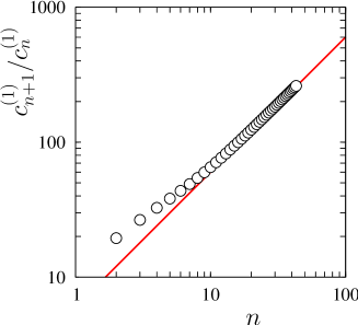
Figure 4: Illustrating the growth of the perturbation coefficients $c^{(1)}_{n}$ with increasing order $n$ for the first Lyapunov exponent, $\Gamma=2$. Shown is the ratio $c^{(1)}_{n+1}/c^{(1)}_{n}$ as a function of $n$. The solid line is the asymptotic relation $c^{(1)}_{n+1}/c^{(1)}_{n}=6\,n$, consistent with $c^{(1)}_{n}\sim C\,6^{n}\,(n-1)!$, for some constant $C$.

for some constant $C$. This factorial growth is typical of an asymptotic series [33]. We find that $S=1/6$, independent of $j$ and $\Gamma$. Figure  4 shows the growth of $c_{n}^{(1)}$ for $\Gamma=2$.

There are rather few concrete physical problems for which perturbation expansion coefficients are available to high order: most studies are concerned with quantum-mechanical problems which are perturbations of a harmonic oscillator, such as [32]. Here we do have the perturbation series coefficients to high order, for the same underlying reason: we used the algebra of harmonic-oscillator raising and lowering operators to compute matrix elements exactly.

Methods for treating divergent series are discussed in [33] and [34], assuming that the expansion can be pursued to high order. Here we use Padé-Borel summation, similar to an approach used to sum the perturbation series of certain one-dimensional quantum-mechanical anharmonic oscillators [32]. We evaluate the ‘Borel sum’

$$B_{j}(\epsilon^{2})=\sum_{n=1}^{n_{\rm max}}\frac{c_{n}^{(j)}}{n!}\epsilon^{2n}$$ (92)

where $n_{\rm max}$ is the number of terms available. The sum of the series is then taken to be

$$\lambda_{j}/\gamma=\mbox{Re}\int_{\cal C}{\rm d}t\,B_{j}(\epsilon^{2}\,t){\rm e}^{-t}$$ (93)

where ${\cal C}$ is a suitable curve in the complex plane. Assuming that the Borel sum has a finite radius of convergence, the function may be approximated by Padé approximants of order $N/M$, $P_{N/M}(\epsilon^{2}t)$ [35]. Here $N$ and $M$ are the orders of the numerator and denominator polynomials, respectively and $N+M\leq n_{\rm max}$, where $n_{\rm max}$ is the number of coefficients available.

The integral in (93) is evaluated numerically. If the Padé approximants to $B_{j}(\epsilon^{2}t)$ have poles on the positive real axis, the integration path in (93) is taken to be a ray in the upper right quadrant in the complex plane.

Results of Padé-Borel summation of the series for $\lambda_{1}$ in the incompressible case ($\Gamma=2$) are shown in figure 5a for $N=M=5,10,15,20,23$. The summation results are in good agreement with numerical results for $\lambda_{1}$ obtained as described in section 3.2. For the first Lyapunov exponent, we obtained higher-order coefficients using the method described in [21] (which is particularly efficient but also restricted to calculating the maximal exponent): in this case $n_{\rm max}=47$. We conclude that the Padé-Borel approach works very well for the largest Lyapunov exponent.

Figure 5b shows results for the first and second Lyapunov exponents for $\Gamma=1$, representing a flow field with both solenoidal and compressible components. For the maximal Lyapunov exponent, $\lambda_{1}$, Padé-Borel summation gives very good agreement with the numerical results. For the second Lyapunov exponent, inspection of the coefficients (6.3) shows that for $\Gamma=1$, $c_{l}^{(2)}=-c_{l}^{(1)}$, in other words, the perturbation coefficients for $\lambda_{1}+\lambda_{2}$ vanish identically for $\Gamma=1$. However direct numerical simulations show that $\lambda_{1}+\lambda_{2}$ is not equal to zero when $\Gamma=1$. The WKB analysis summarised in section 7 gives rise to the hypothesis that there may be a non-analytical contribution to the Lyapunov exponents of the form $C_{j}(\Gamma,\epsilon)\exp(-1/6\epsilon^{2})$ which has to be added to the Padé-Borel approximation. Figure 5b shows that this is indeed the case for the second Lyapunov exponent for $\Gamma=1$: adding $C\,\exp(-1/6\epsilon^{2})$ (with $C=0.79$ a fitted constant) to the Padé-Borel sum for $\lambda_{2}$ (solid line) gives very good agreement with the numerical data. This observation shows that there are contributions to the Lyapunov exponents which are not captured by a simple application of the Borel-Padé summation technique.

Figure 6 shows a comparison of the results of Borel-Padé summation with Monte-Carlo simulations of all three of the three Lyapunov exponents for $\Gamma=2$ (incompressible flow). Here we used the coefficients given in section 6.2 with $n_{\rm max}=7$. The results for the first Lyapunov exponent show excellent agreement, as mentioned above. Those for the second exponent show a systematic deviation for larger values of $\epsilon$. The results for the third exponent show some instability upon changing the number of terms included in the Borel sum, implying that more terms are required to achieve a convergent result.

We conclude that the Borel-Padé summation gives very satisfactory results for small values of $\epsilon$, but for large $\epsilon$ there are systematic deviations which are not yet understood. These appear to be associated with non-analytic contributions of the form $\exp(-\Phi^{\ast}/\epsilon^{2})$.

6.5 Relation to clustering

A major motivation for calculating the Lyapunov exponents is to evaluate the dimension deficit $\Delta$ (defined by equation (1)) and hence the Lyapunov dimension, $d_{\rm L}=3-\Delta$. To lowest order in $\epsilon$, equations (89) and (6.3) imply that

$$\lambda_{1}/\gamma=(-1+2\Gamma)\epsilon^{2}\,,\hskip 14.22636pt\lambda_{2}/\gamma=(-2+\Gamma)\epsilon^{2}\,,\hskip 14.22636pt\lambda_{3}/\gamma=-3\,\epsilon^{2}\ .$$ (94)

In figure 3 a, b, and c these expressions are shown as dashed lines. Equations (94) imply that in for an incompressible flow ($\Gamma=2$), the sum $\lambda_{1}+\lambda_{2}+\lambda_{3}$ vanishes in the limit of $\epsilon\rightarrow 0$, and so does $\Delta$, defined in (1). This reflects that in the absence of inertial effects, an incompressible flow cannot give rise to density fluctuations. The leading-order behaviour of the dimension deficit is

$$\Delta = \frac{3\Gamma-6}{2\Gamma-1}+\frac{54-54\,\Gamma+21\,\Gamma^{2}}{2\Gamma-1}\,\epsilon^{2}+O(\epsilon^{4})\ .$$ (95)

In the incompressible case this gives $\Delta=10\,\epsilon^{2}$ for small $\epsilon$.

Figure 1a shows numerical results for $\Delta$ as a function of $\epsilon$ for incompressible flow, including the asymptotic approximation (95). When the numerical results were re-plotted in figure 1b, we used the relation ${\rm St}=\epsilon^{2}/0.256^{2}$, with the factor chosen to give a good agreement as judged by eye.

Figure 6b shows results for the dimension deficit $\Delta$ obtained from Padé-Borel summations for the Lyapunov exponents shown in figure 6a, using equation (1). For small values of $\epsilon$ the agreement is excellent. Despite shortcomings of the Borel summations for $\lambda_{2}$ and $\lambda_{3}$ mentioned above, we observe satisfactory agreement between the theory and results of computer simulations for all values of $\epsilon$ where $\Delta$ is positive. In summary, Padé-Borel summation of the series (90) provides a satisfactory theoretical description of the dimension deficit $\Delta$. The maximal value of $\Delta$ obtained here (and in [4]) is in good agreement with direct numerical simulations of particles suspended in a Navier-Stokes flow (see figure 1).

7 WKB analysis

In this section we discuss the stationary solution of the Fokker-Planck equation (54) by means of a WKB method, along the lines discussed in [36]. This gives an indication as to the interpretation of the non-analytic contributions to the Lyapunov exponents of the form $\exp(-\Phi/\epsilon^{2})$ which were considered in section 6. A precise evaluation of these contributions is beyond the scope of existing methods.

It is convenient to re-scale the variables $x_{i}$ in (54) using $x_{i}^{\prime}=x_{i}\,\epsilon$. The stationary Fokker-Planck equation for $P(\mbox{\boldmath$x$}^{\prime})$ is then

$$\nabla^{\prime}\cdot\bigl{[}(-\mbox{\boldmath$v$}^{\prime}+\epsilon^{2}{\bf D}\mbox{\boldmath$\nabla$}^{\prime})P(\mbox{\boldmath$x$}^{\prime})\bigr{]}=0$$ (96)

with $v_{i}^{\prime}=-x_{i}^{\prime}-\sum_{jk}V_{ijk}x_{j}^{\prime}x_{k}^{\prime}$. Equation (96) indicates why the odd orders of the perturbation series developed in section 6 vanish: because this equation contains $\epsilon^{2}$ rather than $\epsilon$, expansion of any quantity as a power series must be a series in powers of $\epsilon^{2}$.

In the remainder of this section we drop the primes and make the WKB ansatz [35]

$$P(\mbox{\boldmath$x$})=A\exp\left[-\frac{1}{\epsilon^{2}}\left(\Phi(\mbox{\boldmath$x$})+\epsilon^{2}\Psi(\mbox{\boldmath$x$})+\cdots\right)\right]$$ (97)

(where $A$ is a normalisation factor). Our objective is to determine the nature of the function $\Phi$ in (97). Inserting this into (96) and keeping only the lowest-order terms in $\epsilon$ gives

$$\mbox{\boldmath$v$}\cdot\mbox{\boldmath$\nabla$}\Phi+\mbox{\boldmath$\nabla$}\Phi\cdot{\bf D}\mbox{\boldmath$\nabla$}\Phi=0\ .$$ (98)

This has the form of a Hamilton-Jacobi equation [36]. Recall that given a Hamiltonian $H(\mbox{\boldmath$x$},\mbox{\boldmath$p$})$ the Hamilton-Jacobi equation for the action $\Phi(\mbox{\boldmath$x$},E)$ is

$$H(\mbox{\boldmath$x$},\mbox{\boldmath$\nabla$}\Phi)=E\ .$$ (99)

The Hamilton-Jacobi equation is solved by finding the classical trajectories which are solutions of Hamilton’s equations of motion. The function $\Phi(\mbox{\boldmath$x$},E)$ is then obtained by integration along the classical trajectory

$$\Phi(\mbox{\boldmath$x$},E)=\int_{0}^{t(\mbox{\boldmath$\scriptstyle x$},\scriptstyle E)}\!\!\!{\rm d}t\ \dot{\mbox{\boldmath$x$}}\cdot\mbox{\boldmath$p$}\ .$$ (100)

In our case, $E=0$ and the Hamiltonian is

$$H(\mbox{\boldmath$x$},\mbox{\boldmath$p$})=\mbox{\boldmath$v$}(\mbox{\boldmath$x$})\cdot\mbox{\boldmath$p$}+\mbox{\boldmath$p$}\cdot{\bf D}\,\mbox{\boldmath$p$}$$ (101)

and (using the fact that ${\bf D}$ is a symmetric matrix) Hamilton’s equations of motion are

$$\dot{\mbox{\boldmath$x$}}=\frac{\partial H}{\partial\mbox{\boldmath$p$}}=\mbox{\boldmath$v$}(\mbox{\boldmath$x$})+2{\bf D}\,\mbox{\boldmath$p$}\ ,\ \ \ \dot{\mbox{\boldmath$p$}}=-\frac{\partial H}{\partial\mbox{\boldmath$x$}}=-{\bf F}\,\mbox{\boldmath$p$}$$ (102)

where the matrix ${\bf F}$ has components $F_{ij}=\partial v_{i}/\partial x_{j}$. Close to the origin, $\Phi(\mbox{\boldmath$x$})$ is expected to be approximately $\Phi_{0}(\mbox{\boldmath$x$})=\frac{1}{2}\mbox{\boldmath$x$}\cdot\bf{D}\,\mbox{\boldmath$x$}$, in agreement with the Gaussian approximate solution (57). The appropriate initial conditions for the trajectories are therefore infinitesimally close to the origin in $x$-$p$-space with initial condition $\mbox{\boldmath$p$}=\mbox{\boldmath$\nabla$}\Phi(\mbox{\boldmath$x$})=\mbox{\boldmath$x$}$.

Singular points of $\Phi(\mbox{\boldmath$x$})$ are points $\mbox{\boldmath$x$}^{\ast}$ where $\mbox{\boldmath$\nabla$}\Phi=\mbox{\boldmath$0$}$. Consider a trajectory from the origin passing through a singular point $\mbox{\boldmath$x$}^{\ast}$. At this point $\mbox{\boldmath$\nabla$}\Phi$ vanishes and consequently also $p$. From this point onwards, $\dot{\mbox{\boldmath$p$}}=\mbox{\boldmath$p$}=0$ and after reaching the singular point the dynamics is thus advective, $\dot{\mbox{\boldmath$x$}}=\mbox{\boldmath$v$}(\mbox{\boldmath$x$})$, with $\Phi$ remaining constant at $\Phi^{\ast}=\Phi(\mbox{\boldmath$x$}^{\ast})$. Singular points are expected to give rise to non-analytic behaviour of the Lyapunov exponents of the form $\exp(-\Phi^{\ast}/\epsilon^{2})$.

There is a trajectory of equations (102) for which all of the coordinates except $x_{1}$ are zero, for which there is a singular point at $x_{1}^{\ast}=-1$ with action $\Phi^{\ast}=\Phi(x_{1}^{\ast})=1/6$. We can therefore expect non-analytic contributions to the Lyapunov exponents of the form $F\exp(-1/6\epsilon^{2})$, where $F$ may have an algebraic dependence upon $\epsilon$.

The formation of caustics is associated with escape of the Langevin trajectory to infinity. The Langevin equations have an attractive fixed point at $\mbox{\boldmath$x$}={\bf 0}$, but particles that diffuse sufficiently far from this fixed point will escape to infinity. We expect that the escape rate contains a factor $\exp[-\Phi^{\ast}/\epsilon^{2}]$, where $\Phi^{\ast}$ is the action of a trajectory to a singular point. We find that the rate of caustic formation is of the form

$$J^{\prime}\sim J^{\prime}_{0}\exp(-\Phi^{\ast}_{\rm caustic}/\epsilon^{2})$$ (103)

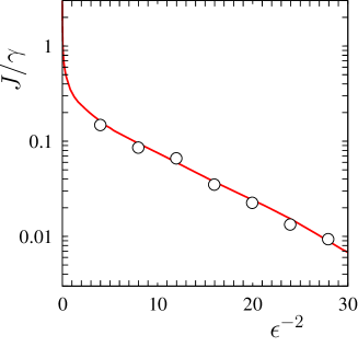
Figure 7: Rate of caustic formation $J^{\prime}=J/\gamma$ as a function of $\epsilon$, for $\Gamma=2$, Monte-Carlo simulations of the Langevin equation (44 - 48), solid red line, and numerical data obtained as described in section 3.2 ($\circ$). The results are asymptotic to $J^{\prime}=C\exp(-\Phi_{\rm caustic}/\epsilon^{2})$ in the limit as $\epsilon\to 0$, with $C\approx 0.28$ and $\Phi_{\rm caustic}\approx 0.125$ (dashed line).

Numerical results confirming this expectation are illustrated in figure 7, which shows that the action associated with the formation of caustics is $\Phi^{\ast}_{\rm caustic}\approx 0.125$.

8 Advective approximation

In the remaining two sections we discuss the overdamped limit $\Omega\gg 1$ and consider how this connects with our results for the underdamped limit described in sections 3 to 7. A surprising fact is that the leading-order formulae for the expansion of the Lyapunov exponents in $\kappa$ are identical in the limits $\Omega\ll 1$ and $\Omega\gg 1$ (although the higher-order terms differ). When $\Omega\gg 1$ the particles are advected by the flow. However, we show that when $\Omega\ll 1$, despite the fact that the particles are not advected, the equations determining their separation are identical to those of advected particles in the limit $\epsilon\to 0$. It is this advective approximation which is discussed in this section.

In the advective limit it is of interest to compute the sum of the three Lyapunov exponents for particles suspended in an incompressible fluid beyond the leading-order approximation. This case is important because its sign determines whether particles in an incompressible flow cluster. The result for purely advected particles is zero, so that a theory going beyond the advective approximation is required. This special case is considered in section 9.

This section is structured as follows. First in section 8.1 we discuss the advective approximation and the conditions for its validity. We also show that the Lyapunov exponents can be obtained from an Itô type Brownian process. The Lyapunov exponents of this process were calculated by Le Jan [13], using a notation and terminology which are difficult to relate to our own. In section 8.2 we calculate the Lyapunov exponents using a simpler method, expressed in our own notation. We calculate the leading-order expressions for the Lyapunov exponents for the model with force statistics defined by equation (35), considered as an expansion in $\kappa$, showing that these are identical when $\Omega\gg 1$ to those expressions obtained in section 6 when $\Omega\ll 1$.

8.1 Brownian advection model

Consider the linearised equations of motion. These can be integrated to give

$$\delta\mbox{\boldmath$r$}(\Delta t)-\delta\mbox{\boldmath$r$}(0)={1\over{m}}\int_{0}^{\Delta t}{\rm d}t_{1}\ \delta\mbox{\boldmath$p$}(t_{1})$$ (104)

and

$$\delta\mbox{\boldmath$p$}(t_{1})=\int_{-\infty}^{t_{1}}{\rm d}t_{2}\ \exp[-\gamma(t_{1}-t_{2})]\,{\bf F}(\mbox{\boldmath$r$}(t_{2}),t_{2})\,\delta\mbox{\boldmath$r$}(t_{2})\ .$$ (105)

We now consider the mean and variance of the displacement (104).

Mean value of displacement

Combining these expressions, writing the result in component form, and expanding the functions in the second integral about $\mbox{\boldmath$r$}(0)$, we obtain

$$\delta r_{\mu}(\Delta t)-\delta r_{\mu}(0) = {1\over{m}}\sum_{\nu}\int_{0}^{\Delta t}{\rm d}t_{1}\ \int_{-\infty}^{t_{1}}{\rm d}t_{2}\ \exp[-\gamma(t_{1}-t_{2})]\,F_{\mu\nu}(\mbox{\boldmath$r$}(0),t_{2})\delta r_{\nu}(0)$$ (106)

$$+{1\over{m^{2}}}\sum_{\nu\lambda}\int_{0}^{\Delta t}{\rm d}t_{1}\int_{-\infty}^{t_{1}}{\rm d}t_{2}\ \exp[-\gamma(t_{1}-t_{2})]\int_{0}^{t_{2}}{\rm d}t_{3}\int_{-\infty}^{t_{3}}{\rm d}t_{4}\ \exp[-\gamma(t_{3}-t_{4})]$$

$$\times\biggl{[}{\partial^{2}f_{\mu}\over{\partial r_{\nu}\partial r_{\lambda}}}(\mbox{\boldmath$r$}(0),t_{2})\,f_{\lambda}(\mbox{\boldmath$r$}(0),t_{4})+{\partial f_{\mu}\over{\partial r_{\nu}}}\bigl{(}\mbox{\boldmath$r$}(0),t_{2}\bigr{)}\,{\partial f_{\nu}\over{\partial r_{\lambda}}}(\mbox{\boldmath$r$}\bigl{(}0),t_{4}\bigr{)}\biggr{]}\delta r_{\nu}(0)\delta r_{\lambda}(0)$$

$$+O(f^{3})\ .$$

This approximation is valid when the absolute displacement $\Delta\mbox{\boldmath$r$}$ during time $\Delta t$ is small compared to the correlation length: $|\Delta\mbox{\boldmath$r$}(\Delta t)|\ll\xi$. The force is derived from potentials, as specified by equation (34). The potentials $\phi$ and $A_{\mu}$ have statistics (given by (35)) which are spatially homogeneous and isotropic. Consider the correlation function of two such quantities $A$ and $B$ which have spatially homogeneous statistics. The following relation holds between correlation functions involving derivatives:

$$\biggl{\langle}{\partial A\over{\partial r_{\lambda}}}(\mbox{\boldmath$r$},t)B(\mbox{\boldmath$r$}^{\prime},t)+A(\mbox{\boldmath$r$},t){\partial B\over{\partial r^{\prime}_{\lambda}}}(\mbox{\boldmath$r$}^{\prime},t^{\prime})\biggr{\rangle}=0\ .$$ (107)

Applying this relation to (106), with $\partial f_{\mu}/\partial r_{\nu}$ and $f_{\nu}$ playing the role of the functions $A$ and $B$, we see that

$$\langle\delta\mbox{\boldmath$r$}(\Delta t)-\delta\mbox{\boldmath$r$}(0)\rangle=O(\Delta t^{2})\ .$$ (108)

Variance of displacement

The variance of (104) is

$$\langle[\delta\mbox{\boldmath$r$}(\Delta t)-\delta\mbox{\boldmath$r$}(0)]^{2}\rangle=\Delta t{1\over{m^{2}}}\int_{-\infty}^{\infty}{\rm d}t\ \langle\delta\mbox{\boldmath$p$}(t)\cdot\delta\mbox{\boldmath$p$}(0)\rangle+O(\Delta t^{2})\,.$$ (109)

The correlation function of the components of the momentum difference is

$$\langle\delta p_{\mu}(t)\delta p_{\mu^{\prime}}(0)\rangle \sim \sum_{\nu\nu^{\prime}}\int_{-\infty}^{0}{\rm d}t_{1}\int_{-\infty}^{0}{\rm d}t_{2}\ \exp[\gamma(t_{1}+t_{2})]$$ (110)

$$\times \biggl{\langle}{\partial f_{\mu}\over{\partial r_{\nu}}}(\mbox{\boldmath$r$}(t+t_{1}),t+t_{1}){\partial f_{\mu^{\prime}}\over{\partial r_{\nu^{\prime}}}}(\mbox{\boldmath$r$}(t_{2}),t_{2})\biggr{\rangle}\,\delta r_{\nu}(0)\delta r_{\nu^{\prime}}(0)\ .$$

We consider the evaluation of the momentum correlation function (110) in successively the underdamped and overdamped limits. In both cases we assume that the displacement $\Delta\mbox{\boldmath$r$}$ during the relevant correlation time is small compared to $\xi$. In the underdamped case, $\Omega\ll 1$, we can approximate the correlation function appearing in (110) by a delta function multiplied by a weight

$$\biggl{\langle}{\partial f_{\mu}\over{\partial r_{\nu}}}(\mbox{\boldmath$r$}(t_{1}),t_{1}){\partial f_{\mu^{\prime}}\over{\partial r_{\nu^{\prime}}}}(\mbox{\boldmath$r$}(t_{2}),t_{2})\biggr{\rangle}\sim 2\,{\cal D}_{\mu\nu,\mu^{\prime}\nu^{\prime}}\,\delta(t_{1}-t_{2})$$ (111)

where the coefficients ${\cal D}_{\mu\nu,\mu^{\prime}\nu^{\prime}}$ are defined by equation (33). Using this approximation to simplify (110) we find

$$\langle\delta p_{\mu}(t)\delta p_{\mu^{\prime}}(0)\rangle={1\over\gamma}\exp(-\gamma|t|)\sum_{\nu\nu^{\prime}}{\cal D}_{\mu\nu,\mu^{\prime}\nu^{\prime}}\,\delta r_{\nu}(0)\delta r_{\nu^{\prime}}(0)\ ,\ \ \ {\rm(underdamped\ case)},\ \Omega\ll 1\ .$$ (112)

In the case where $\gamma\tau\gg 1$, the integral (110) is dominated by the region $t_{1}\sim t_{2}\sim 0$, and we obtain

$$\langle\delta p_{\mu}(t)\delta p_{\mu^{\prime}}(0)\rangle=\sum_{\nu\nu^{\prime}}{1\over{\gamma^{2}}}\biggl{\langle}{\partial f_{\mu}\over{\partial r_{\nu}}}(\mbox{\boldmath$r$}(t),t){\partial f_{\mu^{\prime}}\over{\partial r_{\nu^{\prime}}}}(\mbox{\boldmath$r$}(0),0)\biggr{\rangle}\,\delta r_{\nu}(0)\delta r_{\nu^{\prime}}(0)\ ,\ \ \ {\rm(overdamped\ case)},\ \Omega\gg 1\ .$$ (113)

Thus we find that the momentum correlation functions are different in the underdamped and overdamped cases. However, when we evaluate the variance of the change in spatial separation using (109), we find the same result in both limits:

$$\langle[\delta\mbox{\boldmath$r$}(\Delta t)-\delta\mbox{\boldmath$r$}(0)]^{2}\rangle={2\Delta t\over{m^{2}\gamma^{2}}}\sum_{\mu\nu\nu^{\prime}}{\cal D}_{\mu\nu,\mu\nu^{\prime}}\,\delta r_{\nu}(0)\delta r_{\nu^{\prime}}(0)\ .$$ (114)

Equations (108) and (114) give the statistics of the change in the particle separation after a short time $\Delta t$. This result is valid both when $\Omega\gg 1$ (overdamped limit) and when $\Omega\ll 1$ (underdamped limit), provided that the particle displacement is sufficiently small . In both cases we estimate the displacement as $|\Delta\mbox{\boldmath$r$}(\Delta t)|\approx\sqrt{D\Delta t}$, where $D\approx u^{2}\tau$ is the spatial diffusion constant. In the underdamped case the correlation time is $O(1/\gamma)$, and the requirement that $\Delta\mbox{\boldmath$r$}(\gamma^{-1})\ll\xi$ gives the condition $u\sqrt{\tau}/\xi\sqrt{\gamma}\ll 1$ that is $\epsilon\ll 1$. In the overdamped limit (108) and (114) are always valid when $\kappa\ll 1$.

Relation to advective model

Equations (108) and (114) imply that both in the overdamped limit and in the underdamped limit when $\epsilon\ll 1$, the dynamics may be approximated by a random advection model. In this model the displacement of a particle during time $\Delta t$ is a function only of the position of the particle at time $t$, and not its momentum: we write the displacement at $t=n\Delta t$ as

$$\mbox{\boldmath$r$}(t+\Delta t)=\mbox{\boldmath$r$}(t)+\mbox{\boldmath$w$}_{n}(\mbox{\boldmath$r$})\Delta t$$ (115)

The values of $\mbox{\boldmath$w$}_{n}$ at successive time steps are uncorrelated and average to zero, but $\mbox{\boldmath$w$}_{n}(\mbox{\boldmath$r$})$ is a smoothly varying function of position, so that nearby particles follow similar paths in this random advection model. The spatial correlation of $\mbox{\boldmath$w$}_{n}(\mbox{\boldmath$r$})$ at equal times ($n=n^{\prime}$) is determined by that of $\mbox{\boldmath$u$}(\mbox{\boldmath$r$},t)$.

The separation $\delta\mbox{\boldmath$r$}$ of two trajectories satisfies

$$\delta\mbox{\boldmath$r$}(t+\Delta t)=[{\bf I}+{\bf M}_{n}]\delta\mbox{\boldmath$r$}(t)$$ (116)

where ${\bf I}$ is the identity matrix and where ${\bf M}_{n}$ is a matrix with elements $({\bf M}_{n})_{\mu\nu}=(\partial(\mbox{\boldmath$w$}_{n})_{\mu}/\partial r_{\nu})\delta t$. The elements of this matrix are assumed to have mean value zero and to have diffusive increments: for consistency with (114) we write

$$\langle({\bf M}_{n})_{\mu\nu}\rangle=0$$ (117)

$$\langle({\bf M}_{n})_{\mu\nu}({\bf M}_{n^{\prime}})_{\mu^{\prime}\nu^{\prime}}\rangle={2\over{m^{2}\gamma^{2}}}\delta_{nn^{\prime}}{\cal D}_{\mu\nu,\mu^{\prime}\nu^{\prime}}\Delta t\ .$$ (118)

Equations (115) to (118) define an Itô type stochastic process. It is a surprising feature that an Itô rather than a Stratonovich type equation [37] arises as a stochastic approximation to a system of continuous differential equations.

Note that we do not claim that the particles are always simply advected by the flow $\mbox{\boldmath$u$}(\mbox{\boldmath$r$},t)$ when $\Omega\ll 1$ and $\epsilon\ll 1$: in the overdamped case this is true, but in the underdamped case they are not advected. The statement is that the particle separations behave as if the particles were being advected, according to the simple model (115).

8.2 Lyapunov exponents of Brownian advection model

The Lyapunov exponents for processes of the type defined by (115) to (118) were obtained by LeJan [13]. Here we calculate these Lyapunov exponents using a different and much simpler approach, facilitating direct comparison with the coefficients in equation (6.3).

First Lyapunov exponent

The Lyapunov exponent $\lambda_{1}$ is obtained by considering the magnitude of the separations $\delta r(t)=|\delta\mbox{\boldmath$r$}(t)|$, at successive time steps:

$$\lambda_{1}={1\over{\Delta t}}\biggl{\langle}\log_{\rm e}\biggl{(}{\delta r(t+\Delta t)\over{\delta r(t)}}\biggr{)}\biggr{\rangle}\ .$$ (119)

From (116) we obtain (from here on we drop the subscript labeling the time step on the matrix ${\bf M}_{n}$)

$$\delta r^{2}(t+\Delta t)=\delta r^{2}(t)\,{\bf n}_{1}\cdot({\bf I}+{\bf M}+{\bf M}^{T}+{\bf M}^{T}{\bf M})\,{\bf n}_{1}$$ (120)

where ${\bf n}_{1}$ is a unit vector such that $\delta\mbox{\boldmath$r$}=\delta r{\bf n}_{1}$. Anticipating that two other unit vectors will be defined in due course, and writing

$$M_{\mu\nu}^{\prime}={\bf n}_{\mu}\cdot{\bf M}\,{\bf n}_{\nu}$$ (121)

we obtain

$${\delta r(t+\Delta t)\over{\delta r(t)}} = \sqrt{1+2M^{\prime}_{11}+({\bf M}^{T}{\bf M})^{\prime}_{11}}$$

$$= 1+M^{\prime}_{11}-{\textstyle{1\over 2}}{M^{\prime}}_{11}^{2}+{\textstyle{1\over 2}}({\bf M}^{T}{\bf M})^{\prime}_{11}+O(M^{3})$$

$$\log_{\rm e}\biggl{(}{\delta r(t+\Delta t)\over{\delta r(t)}}\biggr{)} = M^{\prime}_{11}-{M^{\prime}}_{11}^{2}+{\textstyle{1\over 2}}({\bf M}^{T}{\bf M})^{\prime}_{11}+O(M^{3})$$ (122)

$$= M^{\prime}_{11}+{\textstyle{1\over 2}}\sum_{\mu}{M^{\prime}}_{1\mu}^{2}-{M^{\prime}}_{11}^{2}+O(M^{3})\ .$$

Taking the expectation value using (117) and (118) we obtain

$$\lambda_{1}={1\over{m^{2}\gamma^{2}}}\biggl{[}\sum_{\mu=1}^{d}{\cal D}_{\mu 1\mu 1}-2{\cal D}_{1111}\biggr{]}$$ (123)

where $d$ is the number of space dimensions. Finally we relate this expression for the Lyapunov exponent to the results of section 6, showing agreement with the lowest-order terms of the expansions $\epsilon$. Using the properties of the elements ${\cal D}_{\mu\nu\mu^{\prime}\nu^{\prime}}$ discussed in section 4, (123) gives

$$\lambda_{1}=\gamma{{\cal D}_{1}\over{m^{2}\gamma^{3}}}(2\Gamma-1)=\gamma\epsilon^{2}(2\Gamma-1)$$ (124)

(here we used the fact that ${\cal D}_{1313}={\cal D}_{1212}\equiv{\cal D}_{2}\equiv\Gamma{\cal D}_{1}$). This agrees with the leading-order term in the expansion (89), (6.3).

Second Lyapunov exponent

For the second Lyapunov exponent we follow an approach analogous to that of section 3: we consider two vectors $\delta\mbox{\boldmath$r$}_{1}=\delta r{\bf n}_{1}$ and $\delta\mbox{\boldmath$r$}_{2}=\delta\mbox{\boldmath$r$}_{1}+\delta r\delta\theta{\bf n}_{2}$, where ${\bf n}_{2}$ is orthogonal to ${\bf n}_{1}$ and where $\delta\theta\ll 1$. A third unit vector is defined by ${\bf n}_{3}={\bf n}_{1}\wedge{\bf n}_{2}$. The area of the parallelogram spanned by the vectors $\delta\mbox{\boldmath$r$}_{1}$ and $\delta\mbox{\boldmath$r$}_{2}$ is $\delta{\cal A}(t)=|\delta\mbox{\boldmath$r$}_{1}(t)\wedge\delta\mbox{\boldmath$r$}_{2}(t)|$. The second Lyapunov exponent may be obtained from the relation

$$\lambda_{1}+\lambda_{2}={1\over{\Delta t}}\biggl{\langle}\log_{\rm e}\biggl{(}{\delta{\cal A}(t+\Delta t)\over{\delta{\cal A}(t)}}\biggr{)}\biggr{\rangle}\ .$$ (125)

We find $\delta{\cal A}(t)=\delta r^{2}\delta\theta$ and

$$\delta{\cal A}(t+\Delta t)=|{\bf n}_{1}\wedge{\bf n}_{2}+\mbox{\boldmath$z$}|$$ (126)

where

$$\mbox{\boldmath$z$}={\bf M}{\bf n}_{1}\wedge{\bf n}_{2}+{\bf n}_{1}\wedge{\bf M}{\bf n}_{2}+{\bf M}{\bf n}_{1}\wedge{\bf M}{\bf n}_{2}\ .$$ (127)

This implies

$$\left(\frac{\delta{\cal A}(t+\Delta t)}{\delta{\cal A}(t)}\right)^{2}=1+2{\bf n}_{3}\cdot\mbox{\boldmath$z$}+\mbox{\boldmath$z$}\cdot\mbox{\boldmath$z$}\ .$$ (128)

It is convenient to express these vectors in terms of components: for example we have ${\bf M}{\bf n}_{1}=M^{\prime}_{11}{\bf n}_{1}+M^{\prime}_{21}{\bf n}_{2}+M^{\prime}_{31}{\bf n}_{3}$ so that ${\bf M}{\bf n}_{1}\wedge{\bf n}_{2}=M^{\prime}_{11}{\bf n}_{3}-M^{\prime}_{31}{\bf n}_{1}$. We find ${\bf n}_{3}\cdot\mbox{\boldmath$z$}=M^{\prime}_{11}+M^{\prime}_{22}+M^{\prime}_{11}M^{\prime}_{22}-M^{\prime}_{21}M^{\prime}_{12}$ and $\mbox{\boldmath$z$}\cdot\mbox{\boldmath$z$}={M^{\prime}}_{31}^{2}+{M^{\prime}}_{32}^{2}+{M^{\prime}}_{11}^{2}+{M^{\prime}}_{22}^{2}+2M^{\prime}_{11}M^{\prime}_{22}+O(M^{3})$. This gives

$$\left(\frac{\delta{\cal A}(t+\Delta t)}{\delta{\cal A}(t)}\right)^{2} = 1+2(M^{\prime}_{11}+M^{\prime}_{22})+2M^{\prime}_{11}M^{\prime}_{22}-2M^{\prime}_{21}M^{\prime}_{12}$$

$$+{M^{\prime}}_{31}^{2}+{M^{\prime}}_{32}^{2}+(M^{\prime}_{11}+M^{\prime}_{22})^{2}+O(M^{3})$$

$${\delta{\cal A}(t+\Delta t)\over{\delta{\cal A}(t)}} = 1+M^{\prime}_{11}+M^{\prime}_{22}-M^{\prime}_{21}M^{\prime}_{12}+M^{\prime}_{11}M^{\prime}_{22}+{\textstyle{1\over 2}}{M^{\prime}}_{31}^{2}+{\textstyle{1\over 2}}{M^{\prime}}_{32}^{2}+O(M^{3})$$

$$\log_{\rm e}{\delta{\cal A}(t+\Delta t)\over{\delta{\cal A}(t)}} = M^{\prime}_{11}+M^{\prime}_{22}-M^{\prime}_{12}M^{\prime}_{21}-{\textstyle{1\over 2}}{M^{\prime}}_{11}^{2}-{\textstyle{1\over 2}}{M^{\prime}}_{22}^{2}+{\textstyle{1\over 2}}{M^{\prime}}_{31}^{2}+{\textstyle{1\over 2}}{M^{\prime}}_{32}^{2}$$

$$+O(M^{3})\ .$$

Using (125), (117) and (118), the sum of the first two Lyapunov exponents is found to be

$$\lambda_{1}+\lambda_{2}={1\over{m^{2}\gamma^{2}}}\bigl{(}{\cal D}_{3131}+{\cal D}_{3232}-{\cal D}_{1111}-{\cal D}_{2222}-2{\cal D}_{2112}\bigr{)}\ .$$ (130)

Expressing (130) in terms of the notation used in section 6, we find

$$\lambda_{1}+\lambda_{2}={1\over{m^{2}\gamma^{2}}}\bigl{(}2{\cal D}_{2}-2{\cal D}_{1}-2{\cal D}_{3}\bigr{)}=\gamma{{\cal D}_{1}\over{m^{2}\gamma^{3}}}(2\Gamma-2-2\sigma)=\gamma\epsilon^{2}(3\Gamma-3)\ .$$ (131)

This gives $\lambda_{2}=\gamma\epsilon^{2}(\Gamma-2)$, which is consistent with the leading-order term of the expansion of $\lambda_{2}$ in (6.3).

Third Lyapunov exponent

The third Lyapunov exponent is determined by considering the sum of the first three Lyapunov exponents, which are obtained from the mean logarithmic derivative of the volume element $\delta{\cal V}(t)$:

$$\lambda_{1}+\lambda_{2}+\lambda_{3}={1\over{\Delta t}}\biggl{\langle}\log_{\rm e}\biggl{(}{{\cal V}(t+\Delta t)\over{\cal V}(t)}\biggr{)}\biggr{\rangle}\ .$$ (132)

We have

$${{\cal V}(t+\Delta t)\over{\cal V}(t)} = {\rm det}({\bf I}+{\bf M})$$

$$\log_{\rm e}\biggl{(}{{\cal V}(t+\Delta t)\over{\cal V}(t)}\biggr{)} = \log_{\rm e}{\rm det}({\bf I}+{\bf M})={\rm tr}\log_{\rm e}({\bf I}+{\bf M})$$ (133)

$$= {\rm tr}\bigl{[}{\bf M}-{\textstyle{1\over 2}}{\bf M}^{2}\bigr{]}+O(M^{3})\ .$$

The sum of the first three Lyapunov exponents is therefore

$$\lambda_{1}+\lambda_{2}+\lambda_{3} = -{\textstyle{1\over 2}}{1\over{\Delta t}}\biggl{\langle}{\rm tr}({\bf M}^{2})\biggr{\rangle}$$ (134)

$$= -\frac{3}{m^{2}\gamma^{2}}\bigl{[}{\cal D}_{1111}+{\cal D}_{1221}+{\cal D}_{1331}\bigr{]}\,.$$

In the notation of section 6, (134) gives

$$\lambda_{1}+\lambda_{2}+\lambda_{3}={-3\over{m^{2}\gamma^{2}}}\bigl{(}{\cal D}_{1}+2{\cal D}_{3}\bigr{)}=-3\gamma\epsilon^{2}(1+2\sigma)=-3(2-\Gamma)\gamma\epsilon^{2}$$ (135)

Subtracting (131) we find $\lambda_{3}=-3\gamma\epsilon^{2}$, which agrees with the leading term of (6.3).

Equation (134) may also be written in the form

$$\lambda_{1}+\lambda_{2}+\lambda_{3} = -\frac{1}{2}\int_{-\infty}^{\infty}{\rm d}t\,\langle{\rm div}\,\mbox{\boldmath$w$}(\mbox{\boldmath$0$},t)\,{\rm div}\,\mbox{\boldmath$w$}(\mbox{\boldmath$0$},0)\rangle\ .$$ (136)

Here $\mbox{\boldmath$w$}(\mbox{\boldmath$r$},t)$ is related to the velocity field $\mbox{\boldmath$w$}_{n}(\mbox{\boldmath$r$})$ in equation (115) by $\mbox{\boldmath$w$}_{n}(\mbox{\boldmath$r$})=\mbox{\boldmath$w$}(\mbox{\boldmath$r$},n\Delta t)$. A similar expression has been quoted by Balkovsky et al. [17].

9 Correction to overdamped limit

In the previous section, the advective approximation of the solution of equation (3) was considered. We showed that whenever $\epsilon\ll 1$, at leading order in $\kappa$ we can apply a model in which the particles are advected by a random flow. The only case where the advective approximation is inadequate in the overdamped limit is the following. Consider the quantity $\Delta$, defined in equation (1). Its sign and magnitude determine whether or not clustering occurs, and to which extent. In the case of an incompressible flow, $\Delta$ vanishes in the advective approximation, because the flow is volume preserving (this also follows from equation (135), noting that $\Gamma=2$ for incompressible flow). In order to compute whether $\Delta$ is positive or negative (which determines whether or not clustering happens) it is thus necessary to go beyond the advective approximation, as explained in the following.

We consider an incompressible flow field $\mbox{\boldmath$u$}(\mbox{\boldmath$r$},t)$. We make use of a result due to Maxey [1] who has derived a ‘synthetic’ velocity field including a correction term which is proportional to $1/\gamma$ and shown that this modified field describes, to leading order, corrections to the purely advective limit. Maxey’s synthetic field was subsequently employed in [16, 38, 17] to study particle-density fluctuations in incompressible fluids in the near-advective limit.

As pointed out by Maxey, this correction term gives rise to a potential component in the synthetic advection field which, according to equation (134), implies that $\Delta>0$. The aim of this section is to evaluate this correction, and to express it in terms of the dimensionless parameters $\kappa$ and $\Omega$.

Integrating (3) one obtains

$$\mbox{\boldmath$p$}(t) = \int_{-\infty}^{t}\!\!{\rm d}t_{1}\ \exp[-\gamma(t-t_{1})]\mbox{\boldmath$f$}(\mbox{\boldmath$r$}(t_{1}),t_{1})$$ (137)

$$= \frac{1}{\gamma}\Big{[}\mbox{\boldmath$f$}(\mbox{\boldmath$r$}(t),t)-\int_{-\infty}^{t}\!\!{\rm d}t_{1}\ \exp[-\gamma(t-t_{1})]\frac{\rm d}{{\rm d}t_{1}}\mbox{\boldmath$f$}(\mbox{\boldmath$r$}(t_{1}),t_{1})\Big{]}$$

ignoring an initial transient. Using $\mbox{\boldmath$f$}=m\gamma\mbox{\boldmath$u$}$ this gives, to leading order in $\Omega^{-1}=(\gamma\tau)^{-1}$

$$\dot{\mbox{\boldmath$r$}}=\mbox{\boldmath$u$}(\mbox{\boldmath$r$}(t),t)-\frac{1}{\gamma}\Big{[}\frac{\partial}{\partial t}\mbox{\boldmath$u$}(\mbox{\boldmath$r$}(t),t)+\big{(}\mbox{\boldmath$u$}(\mbox{\boldmath$r$}(t),t)\cdot\mbox{\boldmath$\nabla$}\big{)}\dot{\mbox{\boldmath$r$}}\Big{]}\ .$$ (138)

As pointed out by Maxey (equation (5.9) in [1]) this equation describes advection in a synthetic velocity field

$$\mbox{\boldmath$v$}=\mbox{\boldmath$u$}-\frac{1}{\gamma}\Bigg{[}\frac{\partial\mbox{\boldmath$u$}}{\partial t}+\big{(}\mbox{\boldmath$u$}\cdot\mbox{\boldmath$\nabla$}\big{)}\mbox{\boldmath$u$}\Bigg{]}\ .$$ (139)

The sum of the Lyapunov exponents for this advection problem are given by (136). Since $\mbox{div}\,\mbox{\boldmath$v$}=\gamma^{-1}\mbox{\boldmath$\nabla$}(\mbox{\boldmath$u$}\cdot\mbox{\boldmath$\nabla$})\mbox{\boldmath$u$}$, we have

$$\lambda_{1}+\lambda_{2}+\lambda_{3}=-\frac{1}{2\gamma^{2}}\int_{-\infty}^{\infty}{\rm d}t\,\Big{\langle}\Big{(}\mbox{\boldmath$\nabla$}\cdot(\mbox{\boldmath$u$}\cdot\mbox{\boldmath$\nabla$})\mbox{\boldmath$u$}\Big{)}_{t}\Big{(}\mbox{\boldmath$\nabla$}\cdot(\mbox{\boldmath$u$}\cdot\mbox{\boldmath$\nabla$})\mbox{\boldmath$u$}\Big{)}_{0}\Big{\rangle}\ .$$ (140)

We will estimate this expression for a particular example, where the correlation function $C(R,t)$ in (35) factorises into a spatial and a time-dependent part: $C(R,t)=C_{0}(R)\Phi(t)$. In the incompressible case where $\nabla\cdot\mbox{\boldmath$u$}=0$, we obtain

$$\lambda_{1}+\lambda_{2}+\lambda_{2}=-\left\langle\left(\sum_{\mu\nu}\frac{\partial u_{\mu}}{\partial r_{\nu}}\frac{\partial u_{\nu}}{\partial r_{\mu}}\right)^{2}\right\rangle\,\frac{1}{2\gamma^{2}}\int_{-\infty}^{\infty}{\rm d}t\,\Phi^{2}(t)\ .$$ (141)

In terms of the characteristic quantities of the flow, we therefore estimate $\lambda_{1}+\lambda_{2}+\lambda_{3}\sim\kappa^{4}/(\Omega^{2}\tau)$. Together with (124) this gives, for $\Omega\gg 1$,

$$\Delta\sim\frac{\kappa^{2}}{\Omega^{2}}\ .$$ (142)

This result should be contrasted with (95), valid for $\Omega\ll 1$, which implies that $\Delta\sim\kappa^{2}/\Omega$. Thus $\Delta$ is given in terms if different combinations of dimensionless parameters $\kappa$ and $\Omega$ for $\Omega\ll 1$ and $\Omega\gg 1$. In the underdamped case, $\Delta$ is obtained as a perturbation expansion in $\epsilon=\kappa\Omega^{-1/2}$. In the overdamped case, by contrast, it is obtained as a perturbation expansion in $\kappa/\Omega$ and $\kappa/\Omega^{2}$. We note that expression (142) is always small in the domain of its validity: $\Omega\gg 1$ and $\kappa<1$. The results of section 6 by contrast, remain valid when $\Delta$ is of order unity.

10 Concluding remarks

10.1 Conclusions

In this paper we have characterised the local properties of the motion of inertial particles in a short-time correlated random flow model. We calculated the Lyapunov exponents using an exact series expansion, and characterised the rate of caustic formation in terms of an escape process.

The results give important new insights into the mechanism for particle clustering. The relevant dimensionless parameter is $\epsilon\sim\kappa\Omega^{-1/2}$, and we find that the dimension deficit is significant when $\epsilon$ is of order unity, reaching a maximum value of $\Delta_{\rm max}\approx 0.35$ at $\epsilon_{\rm max}\approx 0.21$. This contradicts the accepted explanation for particle clustering, based on the centrifuge mechanism, because (when $\kappa\ll 1$) it implies that clustering onto a fractal set can occur when the Stokes number $\Omega^{-1}$ is large. For fully developed turbulent flow, we have $\kappa=O(1)$ so that $\epsilon\sim\Omega^{-1/2}$, and in that case our theory does predict that clustering onto a fractal set occurs when the Stokes number is of order unity. This is consistent with numerical experiments. We cannot exclude the possibility that the centrifuge effect has some relevance, however we note that our theory predicts $\Delta_{\rm max}=0.35$ for the maximal dimension deficit, see figure 1b, also [4]. The value obtained from direct numerical simulations of a Navier-Stokes flow is very similar, $\Delta_{\rm max}=0.4$ [3].

For $\epsilon>\epsilon_{\rm c}\approx 0.33$, the dimension deficit is zero, and the particles will not cluster onto a fractal set. However, as $\epsilon$ increases the rate of caustic formation increases. The particle density can diverge on caustic lines, as described in [20].

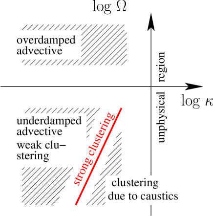
Figure 8: Schematic diagram showing how the behaviour of particles suspended in an incompressible fluid depends upon the parameters $\kappa$ and $\Omega$.

Figure 7 is a schematic illustration of how the unmixing of particles suspended in an incompressible fluid (that is a flow with $\Gamma=2$) depends upon the parameters $\kappa$ and $\Omega$. Instead of clustering being confined to $\Omega\sim 1$, it may occur on a ray in logarithmic parameter space extending into the underdamped region. The solid line in figure 8, $\epsilon\sim\kappa\Omega^{-1/2}=\mbox{const}.$, indicates schematically the critical line where $\Delta$ reaches zero. Above the solid line $\Delta$ is always positive, but tends to zero for small $\epsilon$ as $\Delta=10\epsilon^{2}\sim\kappa^{2}/\Omega$. In section 8 we showed that in the limit of $\epsilon\rightarrow 0$ the dynamics behaves like advection, even if $\Omega\ll 1$.

10.2 Experimental considerations

We make some final comments concerning the situations in which clustering should be observable. The velocity field of fully-developed turbulent flow has a power-law energy spectrum, with an upper and lower cutoff [26]. The smaller length scale is the Kolmogorov length, defined by $\eta=(\nu^{3}/{\cal E})^{1/4}$ where $\nu$ is the kinematic viscosity and ${\cal E}$ is the rate of dissipation per unit mass of fluid. This is the size of the smallest vortices generated by the turbulence. In section 4.3 we show that it is this small length scale $\eta$ which corresponds to the correlation length $\xi$ in our theory. Our results indicate that clustering can certainly occur on a scale smaller than $\xi$, but what happens on larger length scales is less certain.

Lengthscale for clustering

It is not entirely clear whether particles in turbulent flows can exhibit clustering effects on length scales greater than the Kolmogorov length, $\eta$. Particles separated by distances greater than $\eta$ will be separated by Richardson diffusion [39], but that is not necessarily incompatible with some type of clustering. Numerical evidence for such an effect has been presented [7], but the range of Stokes and Reynolds numbers are not sufficiently large to allow clear conclusions. At very small Stokes number, suspended particles are advected and must be mixed to uniform concentration in a turbulent flow. At large Stokes number, however, it is conceivable that particles could be centrifuged away from vortices with length scale $L\gg\eta$ when their rotation period $t_{L}$ is such that the length-dependent Stokes number ${\rm St}_{L}=1/(\gamma T_{L})$ is of order unity [40]. The Kolmogorov theory gives $t_{L}\sim(L^{2}/{\cal E})^{1/3}$. Consequently this picture implies clustering on a length scale $L\sim({\cal E}/\gamma^{3})^{1/2}$.

However, there is an argument which suggests that such large-scale clusters might not form. At large Stokes number, the formation of numerous caustics implies that the velocity field of the suspended particles is multi-valued, so that in the limit ${\rm St}\to\infty$ the suspended particles are expected to behave as a gas [41]. Particles at the same position move with relative speed $\Delta v$; using the Kolmogorov cascade principle, we estimate that the variance of $\Delta v$ is $\langle\Delta v^{2}\rangle\sim{\cal E}/\gamma$ [42]. The motion of the suspended particles is damped at a rate $\gamma$, so that they travel in an approximately straight line for a distance $\Delta v/\gamma$. We see that $\Delta v/\gamma\sim({\cal E}/\gamma^{2})^{1/2}\sim L$. So particles within a cluster of size $L$ travel distances of order $L$ in random directions before their relative motion is damped out. This argument suggests that clustering may be difficult to observe on scales larger than the Kolmogorov length.

Effects of gravity

The Kolmogorov scale is rather insensitive to the value of ${\cal E}$: for $\nu\sim 10^{-5}{\rm m}^{2}{\rm s}^{-1}$ (air at standard atmospheric conditions) and ${\cal E}\sim 1{\rm m}^{2}{\rm s}^{-3}$, we have $\eta\sim 10^{-4}{\rm m}$. Our results concerning the Lyapunov exponents are relevant to clustering of particles on length scales below the Kolmogorov length and therefore describe clustering on very small length scales. They would be relevant to the aggregation of aerosol particles, but it seems unlikely that it could explain the macroscopic clustering observed in the experiments of Fessler and Eaton and [2].

In discussing the conditions under which the clustering effect is observable, we must also consider the effects of gravity. Gravitational effects may be assumed negligible when motion at the terminal velocity moves particles by a distance which is small compared to $\xi$ in time $\tau$. Noting that the terminal velocity is $g/\gamma$, this condition may be written $g\tau^{2}/\xi\Omega\ll 1$. For fully developed turbulence, using the Kolmogorov theory we estimate

$$\frac{g\tau^{2}}{\xi}\sim\frac{g\nu^{1/4}}{{\cal E}^{3/4}}\ .$$ (143)

This quantity is small only for highly energetic turbulence. Thus, in terrestrial applications, direct application of the model to three-dimensional turbulent flows requires very intense turbulence if the effects of gravity are to be neglected.

Acknowledgments. BM acknowledges financial support from Vetenskapsrådet and from the research platform ‘Nanoparticles in an interactive environment’ at Göteborg university.

References

• [1] M. R. Maxey, The gravitational settling of aerosol particles in homogeneous turbulence and random flow fields, J. Fluid Mech. 174, 441-465, (1987).
• [2] J. R. Fessler, J. D. Kulick and J. K. Eaton, Preferential concentration of heavy particles in a turbulent channel flow, Phys. Fluid, 6, 3742, (1994).
• [3] J. Bec, L. Biferale, G. Boffetta, M. Cencini, S. Musachchio and F. Toschi, Lyapunov exponents of heavy particles in turbulence, submitted to Phys. Fluid, (2006), preprint archive: nlin.CD/0606024.
• [4] K. P. Duncan, B. Mehlig, S. Östlund and M. Wilkinson, Clustering in Mixing Flows, Phys. Rev. Lett., 95, 240602, (2005).
• [5] L. P. Wang and M. R. Maxey, Settling Velocity and Concentration Distribution of Heavy Particles in Homogeneous Isotropic Turbulence, J. Fluid. Mech., 256, 27, (1993).
• [6] R. C. Hogan and J. N. Cuzzi, Stokes and Reynolds number dependence of preferential particle concentration in simulated three-dimensional turbulence , Phys. Fluids, 13, 2938-2945, (2001).
• [7] G. Boffeta, F. de Lillo and A. Gamba, Large scale inhomogeneity of inertial partyicles in turbulent flows, Phys. Fluids, 14, L20-L23, (2004).
• [8] J. Sommerer and E. Ott, Particles floating on a random flow: a dynamically comprehensible physical fractal, Science, 359, 334, (1993).
• [9] J. L. Kaplan and J. A. Yorke, in: Functional Differential Equations and Approximations of Fixed Points, eds.: H.-O. Peitgen and H.-O. Walter, Lecture Notes in Mathematics, 730, Springer, Berlin, (1979), p. 204.
• [10] J. Bec, Fractal clustering of inertial particles in random flows , Phys. Fluids, 15, L81-84, (2003).
• [11] J. Bec, Multifractal concentrations of inertial particles in smooth random flows , J. Fluid Mech., 528 255-277 (2005).
• [12] R. J. Kraichnan, Convection of a passive scalar by a quasi-uniform random straining field, J. Fluid. Mech., 64, 737-62, (1974).
• [13] Y. Le Jan, On isotropic Brownian motions, Z. Wahrsch. verw. Gebiete, 70, 609-20, (1985).
• [14] D. Bernard, K. Gawȩdzki and A. Kupiainen, Slow Modes in Passive Advection, J. Stat. Phys., 90, 519-69, (1998).
• [15] G. Falkovich, K. Gawȩdzki and M. Vergassola, Particles and Fields in Fluid Turbulence, Rev. Mod. Phys., 73, 913-75, (2001).
• [16] T. Elperin, N. Kleeorin and I. Rogachevskii, Self-excitation of fluctuation of inertial particle concentration in turbulent fluid flow, Phys. Rev. Lett., 77, 5373, (1996).
• [17] E. Balkovsky, G. Falkovich and A. Fouxon, Intermittent distribution of inertial particles in turbulent flows, Phys. Rev. Lett., 86, 2790-3, (2001).
• [18] M. Wilkinson and B. Mehlig, The Path Coalescence Transition and its Applications, Phys. Rev. E, 68, 040101, (2003).
• [19] B. Mehlig and M. Wilkinson, Coagulation by Random Velocity Fields as a Kramers Problem, Phys. Rev. Lett, 92, 250602, (2004).
• [20] M. Wilkinson and B. Mehlig, Caustics in Turbulent Aerosols, Europhys. Lett., 71, 186-92, (2005).
• [21] B. Mehlig, M. Wilkinson, K. Duncan, T. Weber and M. Ljunggren, On the aggregation of inertial particles in random flows, Phys. Rev. E, 72, 051104, (2005).
• [22] L. I. Piterbarg, The top Lyapunov exponent for a stochastic flow modelling the upper ocean turbulence, SIAM J. Appl. Math., 62, 777-800, (2001).
• [23] A. Brissaud and U. Frisch, Solving Linear Stochastic Differential Equations, J. Math. Phys., 15, 524, (1974).
• [24] M. Wilkinson, B. Mehlig and V. Bezuglyy, Caustic Activation of Rain Showers, Phys. Rev. Lett., 97, 048501, (2006).
• [25] M. Maxey and J. Riley, Equation of Motion for a Small Rigid Sphere in a Non-Uniform Flow, Phys. Fluids, 26, 883-889, (1983).
• [26] U. Frisch, Turbulence, Cambridge Univeristy Press, (1997).
• [27] G. Falkovich, A. Fouxon and G. Stepanov, Acceleration of Rain Initiation by Cloud Turbulence, Nature, 419, 151-154, (2002).
• [28] M. V. Berry, Singularities in Waves, Les Houches Lecture Series Session XXXV, eds. R. Balian, M. Kléman and J-P. Poirier, North Holland: Amsterdam, 453-543, (1981).
• [29] J. P. Eckmann and D. Ruelle, Ergodic Theory of Chaos and Strange Attractors, Rev. Mod. Phys., 57, 617-656, (1985).
• [30] E. Arvedson, M. Wilkinson, B. Mehlig, and K. Nakamura, Staggered Ladder Spectra, Phys. Rev. Lett. 96, 030601, (2006).
• [31] P. A. M. Dirac, The principles of quantum mechanics, Oxford University Press, (1930).
• [32] S. Graffi, V. Grecchi, and B. Simon, Borel Summability - Application to Anharmonic Oscillator , Phys. Lett. B, 32, 631, (1970).
• [33] R. B. Dingle, Asymptotic expansions: their derivation and interpretation, Academic Press, New York, (1974).
• [34] J. P. Boyd, The Devil’s Invention: Asymtotic, Superasymptotic and Hyperasymptotic Series, Acta Applicandae, 56, 98, (1999).
• [35] C. M. Bender and S. A. Orszag, Advanced mathematical methods for scientists and engineers, McGraw-Hill, New York, (1978).
• [36] M. I. Freidlin and A. D. Wentzell, Random Perturbations of Dynamical Systems, Springer: New York (1984).
• [37] N. G. van Kampen, Stochastic processes in physics and chemistry, North-Holland, Amsterdam, (1992).
• [38] M. B. Pinsky, A. P. Khain, and Z. Levin, The role of the inertia of cloud drops in the evolution of the spectra during drop growth by diffusion, Q. J. R. Meteorol. Soc., 125, 553-581, (1999).
• [39] L. F. Richardson, The role of the inertia of cloud drops in the evolution of the spectra during drop growth by diffusion, Proc. Roy. Soc. Lond., A110, 709-37, (1926).
• [40] G. Falkovich, A. Fouxon and M. Stepanov, in Sedimentation and Sediment Transport, eds: A. Gyr and W. Kinzelbach, Kluwer Academic Publishers, Dordrecht, 2003, pp. 155-158.
• [41] J. Abrahamson, Collision rates of small particles in a vigourouslt turbulent fluid Chem. Eng. Sci., 30, 1371, (1975).
• [42] B. Mehlig, V. Uski and M. Wilkinson, Colliding Particles in Highly Turbulent Flows, nlin.CD/0612008, (2006).
Refer to caption