Ring Intermittency in Coupled Chaotic Oscillators at the Boundary of Phase Synchronization

Abstract

A new type of intermittent behavior is described to occur near the boundary of phase synchronization regime of coupled chaotic oscillators. This mechanism, called ring intermittency, arises for sufficiently high initial mismatches in the frequencies of the two coupled systems. The laws for both the distribution and the mean length of the laminar phases versus the coupling strength are analytically deduced. A very good agreement between the theoretical results and the numerically calculated data is shown. We discuss how this mechanism is expected to take place in other relevant physical circumstances.

Intermittent behavior is an ubiquitous phenomenon in nonlinear science. Its arousal and main statistical properties have been studied and characterized already since long time ago, and different types of intermittency have been classified as types I–III P. Berge, Y. Pomeau, Ch. Vidal (1988); M. Dubois, M. Rubio, P. Bergé (1983) or on–off intermittency N. Platt, E.A. Spiegel, C. Tresser (1993); J.F. Heagy, N. Platt, S.M. Hammel (1994). One of the most general and interesting manifestations of the intermittent behavior can be observed near of the boundary of chaotic synchronization regimes. Indeed, close to the threshold parameter values for which the coupled systems show synchronized dynamics, it is observed that the de-synchronization mechanism involves persistent intermittent time intervals during which the synchronized oscillations are interrupted by the non-synchronous behavior. These pre-transitional intermittencies have been described in details for the case of lag synchronization M.G. Rosenblum, A.S. Pikovsky, J. Kurths (1997); S. Boccaletti, D.L. Valladares (2000); M. Zhan et al (2002) and for generalized synchronization A.E. Hramov, A.A. Koronovskii (2005), and their main statistical properties (following those of the on-off intermittency) have been shown to be common to other relevant physical processes.

As far as intermittency phenomena near the phase synchronization onset are concerned, two types of intermittent behavior have been observed so far A. Pikovsky et al (1997); K.J. Lee et al (1998); S. Boccaletti, E. Allaria, R. Meucci, F.T. Arecchi (2002); E.J. Rosa, E. Ott, M.H. Hess (1998), namely the type-I intermittency and the super-long laminar behavior (so called “eyelet intermittency” A. Pikovsky et al (1997)).

In this Letter we report that a new type of intermittent behavior is observed near the phase synchronization boundary of two unidirectionally coupled chaotic oscillators, when the natural frequencies of the two oscillators are sufficiently different from one another. The system under study is represented by a pair of unidirectionally coupled Rössler systems, whose equations read as

$$\begin{array}[]{ll}\dot{x}_{d}=-\omega_{d}y_{d}-z_{d},&\dot{x}_{r}=-\omega_{r}y_{r}-z_{r}+\varepsilon(x_{d}-x_{r}),\\ \dot{y}_{d}=\omega_{d}x_{d}+ay_{d},&\dot{y}_{r}=\omega_{r}x_{r}+ay_{r},\\ \dot{z}_{d}=p+z_{d}(x_{d}-c),\mbox{}&\dot{z}_{r}=p+z_{r}(x_{r}-c),\\ \end{array}$$ (1)

where $(x_{d},y_{d},z_{d})$ [$(x_{r},y_{r},z_{r})$] are the cartesian coordinates of the drive (the response) oscillator, dots stand for temporal derivatives, and $\varepsilon$ is a parameter ruling the coupling strength. The other control parameters of Eq. (1) have been set to $a=0.15$, $p=0.2$, $c=10.0$, in analogy with previous studies  A.E. Hramov, A.A. Koronovskii (2005); A.E. Hramov, A.A. Koronovskii, O.I. Moskalenko (2005). The $\omega_{r}$–parameter (representing the natural frequency of the response system) has been selected to be $\omega_{r}=0.95$; the analogous parameter for the drive system has been fixed to $\omega_{d}=1.0$. For such a choice of parameter values, both chaotic attractors of the drive and response systems are, at zero coupling strength, phase coherent. Furthermore, the boundary of the phase synchronization regime occur around $\varepsilon_{c}\approx 0.124$.

The instantaneous phase of the chaotic signals $\varphi(t)$ can be therefore introduced in the traditional way, as the rotation angle ${\varphi_{d,r}=\arctan(y_{d,r}/x_{d,r})}$ on the projection plane $(x,y)$ of each system. The presence of the phase synchronization regime can be detected by means of monitoring the time evolution of the instantaneous phase difference, that has to obey the phase locking condition S. Boccaletti et al (2002)

$$|\Delta\varphi(t)|=|\varphi_{d}(t)-\varphi_{r}(t)|<\mathrm{const}.$$ (2)

Below the boundary of the phase synchronization regime, the dynamics of the phase difference $\Delta\varphi(t)$ features time intervals of phase synchronized motion (laminar phases) persistently and intermittently interrupted by sudden phase slips (turbulent phases) during which the value of $|\Delta\varphi(t)|$ jumps up by $2\pi$.

By analyzing the statistics of the laminar phases, it is found that the intermittent type behavior described in Refs.  A. Pikovsky et al (1997); K.J. Lee et al (1998); S. Boccaletti, E. Allaria, R. Meucci, F.T. Arecchi (2002); E.J. Rosa, E. Ott, M.H. Hess (1998); A. Pikovsky et al (1997) takes place only for small differences in the natural frequencies of the drive and response systems. In particular, the eyelet intermittent phenomenon occurs in the range $\omega_{d}=0.90\div 0.98$. As far as large differences in the natural frequencies of the drive and response systems are concerned ($\omega_{d}<0.90$ and $\omega_{d}>0.98$), a novel type of intermittent behavior emerges which differs remarkably from the ones known so far. In the following we will describe the properties of this new type of behavior, that we called ring intermittency, due to the specific dynamical mechanism that produces it.

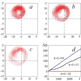
Figure 1: (Color online) The phase trajectory of the response system on the $(x^{\prime},y^{\prime})$-plane rotating around the origin when the coupling parameter strength is selected as (a) $\varepsilon=0.126$ — the phase synchronization regime, (b) $\varepsilon=0.115$ — the ring intermittency and (c) $\varepsilon=0.109$ — the asynchronous dynamics. (d) The dependence of the phase difference $\Delta\varphi(t)$ on the time $t$ for the coupling strength values $\varepsilon$ used in Fig. (a–c).

Let us start with discussing the mechanism at the origin of the arousal of the ring intermittency, and that rules out the scaling laws characterizing this phenomenon. It is well-known that there are two different scenarios for synchronization destruction in a periodic oscillator driven by an external force, corresponding respectively to small and large detunings with the external signal frequency (see, e.g., tutorial A. Pikovsky, M. Rosenblum, J. Kurths (2000)). Under certain conditions (i.e., for the periodically forced weakly nonlinear isochronous oscillator), the complex amplitude method may be used to find the solution describing the oscillator behavior in the form ${u(t)=\mathrm{Re}\,a(t)e^{i\omega t}}$. For the complex amplitude $a(t)$ one obtains averaged (truncated) equations ${\dot{a}=-i\nu a+a-|a|^{2}a-ik}$, where ${\nu}$ is the frequency mismatch, and $k$ is the (renormalized) amplitude of the external force. For the small $\nu$ and large $k$ the stable solution ${a(t)=Ae^{i\phi}=\mathrm{const}}$ corresponds to the synchronous regime, with the synchronization destruction corresponding to the the saddle-node bifurcation on the plane of the complex amplitude. For large frequency mismatches with the decrease of $k$-value the fixed point (stable node) on the complex amplitude plane becomes sequentially a stable focus and an unstable focus (via the Andronov–Hopf bifurcation). In this case the phase synchronization destruction is connected with the limit cycle location on the complex amplitude plane (see A. Pikovsky, M. Rosenblum, J. Kurths (2000) for detail). When the limit cycle starts enveloping the origin, the synchronization regime begins to destroy. Obviously, if one considers the behavior of the synchronized periodic oscillator on the plane $(x^{\prime},y^{\prime})$ rotating with the frequency of the external signal around the origin he observes the stable node for the small values of the frequency detuning and a cycle for the large ones, respectively. These considerations on the rotating plane may be made apparent by using the coordinate transformation ${x^{\prime}=x_{r}\cos\varphi_{d}+y_{r}\sin\varphi_{d}}$, ${y^{\prime}=-x_{r}\sin\varphi_{d}+y_{r}\cos\varphi_{d}}$, where $\varphi_{d}=\varphi_{d}(t)$ is the instantaneous phase of the drive system.

The same effects may be also observed for chaotic oscillators. Indeed, in Fig. 1, a the behavior of the synchronized response oscillator (1) is shown on the plane $(x^{\prime},y^{\prime})$ rotating around the origin in accordance with the phase $\varphi_{d}(t)$ of the drive system when the control parameters $\omega_{d}$ and $\omega_{r}$ are detuned sufficiently. One can see that the phase trajectory on this plane looks like a ring. This effect arises insofar as the Rössler system may be considered as a noise smeared periodic oscillator (see, e.g., A. Pikovsky et al (1997)). Therefore one observes the ring consisting of the phase trajectories, instead of the limit cycle that would occur in the periodic case. It is the case of the large control parameter mismatch that is accompanied by the ring intermittency behavior, while for the small parameter detuning the intermittent type-I as well as the eyelet intermittency are revealed. When the coupling strength $\varepsilon$ gets below the critical value $\varepsilon_{c}$ the phase trajectory on the $(x^{\prime},y^{\prime})$-plane starts enveloping the origin (see Fig. 1, b, the origin is the point of intersection of the dashed lines), and the phase synchronization regime begins to destroy, as a phase slip is observed all the times that the phase trajectory envelops the origin of that plane. As the coupling strength decreases further, the phase trajectory envelops the origin more often, and the phase slips occur more frequently. Finally, when the coupling strength $\varepsilon$ becomes less than $\varepsilon_{t}\approx 0.1097$ the origin is inside the ring (see Fig. 1, c), therefore every rotation of phase trajectory causes a phase slip. So, varying the coupling strength $\varepsilon$ one observes: (i) the phase synchronization regime for ${\varepsilon>\varepsilon_{c}}$, (ii) the intermittent behavior for ${\varepsilon_{t}<\varepsilon<\varepsilon_{c}}$ and (iii) the asynchronous dynamics for ${\varepsilon<\varepsilon_{t}}$ when the phase slips follow each other at approximately equal time intervals $T$, the averaged period of the phase trajectory rotation on the $(x^{\prime},y^{\prime})$-plane (see Fig. 1, d).

Let the probability that the phase trajectory on the rotating $(x^{\prime},y^{\prime})$-plane envelops the origin be ${p=p(\varepsilon)}$. Obviously, $p=0$ if ${\varepsilon>\varepsilon_{c}}$, $p=1$ if ${\varepsilon<\varepsilon_{t}}$ and $0<p<1$ when ${\varepsilon_{t}<\varepsilon<\varepsilon_{c}}$.

In the case of the intermittent behavior (i.e., ${\varepsilon_{t}<\varepsilon<\varepsilon_{c}}$) the probability of the laminar phase with length $T$ to be observed is $P(T)=p^{2}$. This period is determined by the difference of the main frequencies of the drive ($f_{d}$) and response ($f_{r}$) systems and may be calculated as ${T\approx 1/|f_{r}-f_{d}|}$. For the control parameter set mentioned above, we have $T\approx 80$. It is clear that the probability of laminar phases with length $nT$ to arise is $P(nT)=(1-p)^{n-1}p^{2}$. So, the distribution of the laminar phases with generic length $\tau$ should scale as

$$N(\tau)\sim p^{2}(1-p)^{\tau/T-1},\mbox{\quad$\tau>T$}.$$ (3)

Equation (3) may be also rewritten in the form

$$N(\tau)=A\exp(k\tau),\mbox{\quad$\tau>T$}$$ (4)

where $k=(1/T)\ln(1-p)$, $A$ being a normalizing coefficient. Thus, the laminar phase distribution in the ring intermittency obeys an exponential law, with the parameter $k$ being negative due to ${0<p<1}$.

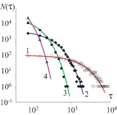
Figure 2: (Color online) The laminar phase length distributions for the different values of the coupling strength $\varepsilon$ and exponential laws (4) corresponding to them. The theoretical curves are shown by lines, the data calculated for two coupled Rössler systems (1) are shown by points. The coupling strength values $\varepsilon$, the probability $p$ and the parameter of the exponential law $k$ have been selected as follows: (1) $\varepsilon=0.123$ ($\circ$), $p=0.06$, $k=-7.7\times 10^{-4}$; (2) $\varepsilon=0.12$ ($\blacklozenge$), $p=0.31$, $k=-4.6\times 10^{-3}$; (3) $\varepsilon=0.115$ ($\blacksquare$), $p=0.65$, $k=-1.3\times 10^{-2}$; (4) $\varepsilon=0.11$ ($\vartriangle$), $p=0.96$, $k=-4.0\times 10^{-2}$.

Let us compare the obtained theoretical law (4) with the results of the numerical calculations of the intermittent behavior of two coupled Rössler systems (1). In Fig. 2 the distribution of the laminar phase lengths are shown for the different values of the coupling strength $\varepsilon$. In the same Figure we report also the exponential fits obeying the law (4). The value of the probability $p(\varepsilon)$ to calculate the coefficient $k$ may be estimated as follows. If the length of the time realization under consideration is $L$ (in our calculations the length of the analyzed time series was $L=2\times 10^{6}$ time units) and $N$ phase slips have been observed during this period, then the probability $p(\varepsilon)$ that the phase trajectory on the rotating $(x^{\prime},y^{\prime})$-plane envelops the origin is $p=NT/L$. E.g., when the coupling strength has been fixed as $\varepsilon=0.12$ (see curve 2 and points $\blacklozenge$ in Fig. 2 for the distribution of the laminar phase lengths) we have observed $N=7,772$ phase slips during the analyzed time series, and therefore the probability $p(\varepsilon)$ was estimated as $p=0.31$. From Fig. 2 one can see an excellent agreement of the numerical data with the theoretical law (4) for the whole range of coupling strength values ${\varepsilon_{t}<\varepsilon<\varepsilon_{c}}$ where the ring intermittency takes place.

Let us now derive the dependence of the mean length $\langle\tau\rangle$ of the laminar phases (i.e., the averaged time interval between two successive phase slips) on the coupling strength $\varepsilon$. From equation (4) one can easily obtain the relationship between the mean length $\langle\tau(\varepsilon)\rangle$ and the probability $p=p(\varepsilon)$

$$\langle\tau\rangle=T-\frac{1}{k}=T-\frac{T}{\ln(1-p)}.$$ (5)

We have numerically observed that, in the coupling strength range ${\varepsilon_{t}<\varepsilon<\varepsilon_{c}}$ where the ring intermittent behavior is observed, the value of the probability $p$ is directly proportional to the deviation of the coupling strength $\varepsilon$ from the critical value $\varepsilon_{c}$, i.e.,

$$p(\varepsilon)\sim\left(\varepsilon_{c}-\varepsilon\right).$$ (6)

Indeed, in Fig. 3 the dependence of the probability $p$ on the deviation of the coupling strength from the critical value ${(\varepsilon_{c}-\varepsilon)}$ is shown. The probability $p(\varepsilon)$ for each value of $\varepsilon$ has been calculated in the same way as it was described above.

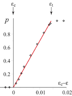
Figure 3: (Color online) The dependence of the probability $p$ that the phase trajectory on the rotating $(x^{\prime},y^{\prime})$-plane envelops the origin on the deviation of the coupling strength from the critical value ${(\varepsilon_{c}-\varepsilon)}$. The points obtained numerically has been shown by symbols $\lozenge$, the linear approximation $p=a(\varepsilon_{c}-\varepsilon)$ (where $a=70$) is shown by a solid line. The critical values $\varepsilon_{c}$ and $\varepsilon_{t}$ of the coupling parameter are shown by arrows. Note, equation (6) is applicable only in the coupling strength range ${\varepsilon_{t}<\varepsilon<\varepsilon_{c}}$.

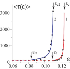
Figure 4: (Color online) The mean length $\langle\tau\rangle$ of the laminar phases vs. $\varepsilon$ calculated numerically ($\lozenge$) for two coupled Rössler systems (1), the theoretical curve (7) (red solid line 1, applicable only in the range $\varepsilon_{t}<\varepsilon<\varepsilon_{c}$ shown by arrows), and the asymptotic ($\varepsilon<\varepsilon_{t}$) value of (5) (red dashed line). The analogous curves (filled dots, blue solid line, blue dashed line) refers to the case of two coupled generators with tunnel diodes of Ref. M.G. Rosenblum, A. Pikovsky, J. Kurths (1997). In this latter case, arrows point to $\varepsilon_{t2}=0.083$ and $\varepsilon_{c2}=0.111$, delimiting the validity range of Eq. (7).

Since the probability $p$ on the coupling strength in the range ${\varepsilon_{t}<\varepsilon<\varepsilon_{c}}$ relates to the coupling strength as ${p(\varepsilon)=(\varepsilon_{c}-\varepsilon)/(\varepsilon_{c}-\varepsilon_{t})}$, one easily obtains that the dependence of the mean laminar phase length on $\varepsilon$ has to scale in the form

$$\langle\tau(\varepsilon)\rangle=T\left(1-\ln^{-1}\left(\frac{\varepsilon-\varepsilon_{t}}{\varepsilon_{c}-\varepsilon_{t}}\right)\right).$$ (7)

Notice that Eq. (7) describes scaling properties for the laminar periods during the ring intermittency that are completely different from those typical of type-I intermittency characterizing the transition to phase locking of periodic oscillators in the presence of noise S. Boccaletti et al (2002), as well as from those arising from the super-long laminar behavior (or eyelet intermittency) characterizing pre-transitional stages of slightly mismatched chaotic oscillators  A. Pikovsky et al (1997); S. Boccaletti, E. Allaria, R. Meucci, F.T. Arecchi (2002). Obviously, equation (7) is correct only in the coupling strength range ${\varepsilon_{t}<\varepsilon<\varepsilon_{c}}$, whereas (5) may be used both below $\varepsilon_{t}$ and above $\varepsilon_{c}$. The mean length $\langle\tau\rangle$ of the laminar phases is about $T$ for values of $\varepsilon$ is below the critical value $\varepsilon_{t}$ (the asynchronous regime where the phase slips follow one another at approximately equal time intervals), and is infinity in the case $\varepsilon>\varepsilon_{c}$. Note also, that $\lim_{\varepsilon\rightarrow+\varepsilon_{t}}\langle\tau(\varepsilon)\rangle=T$ and $\lim_{\varepsilon\rightarrow-\varepsilon_{c}}\langle\tau(\varepsilon)\rangle=+\infty$ in perfect agreement with the system’s behavior at the two boundaries of the intermittency phenomenon ${(\varepsilon_{t};\varepsilon_{c})}$.

Finally, in Fig. 4 the dependence of the mean laminar phase length $\langle\tau\rangle$ on the coupling strength $\varepsilon$ is shown. The points ($\lozenge$) correspond to the calculated mean lengths of the laminar phases and the red solid line 1 reports the theoretical equation (7). Again, one can see a perfect agreement of the theoretical curve with the calculated points. Below the threshold $\varepsilon_{t}$, the calculated mean length of the laminar phases is compared with the asymptotic value $\langle\tau\rangle=T$ (red dashed line). In order to show that our analysis is not limited to the chaotic system (1), we report in the same Figure the analogous curves (filled dots, blue solid line, blue dashed line) obtained for the case of two unidirectionally coupled generators with tunnel diodes described in Ref. M.G. Rosenblum, A. Pikovsky, J. Kurths (1997), where Eq. (7) is valid in the range $\varepsilon_{t2}<\varepsilon<\varepsilon_{c2}$ ($\varepsilon_{t2}=0.083$ and $\varepsilon_{c2}=0.111$). Finally, we would like to stress that the same intermittent scenario can be observed in system (1) for fixed (large enough) values of coupling strength, when varying the parameter mismatch.

In conclusion, we have reported for the first time a new type of intermittency behavior occurring at the onset of phase synchronization regimes of two unidirectionally coupled chaotic oscillators with sufficiently detuned natural frequencies. Such a type of ring intermittency differs remarkably from all the other types of intermittency known so far. It may be observed in a certain range of coupling parameter strengths, where the distribution of the laminar phase lengths obeys an exponential law. The theoretical equation for the dependence of the mean length of the laminar phases on the coupling strength has also been given, and are in perfect agreement with the numerically obtained data. Though the characterization of the new intermittent process has been here explicitly derived at the boundary of phase synchronization of chaotic systems, we expect that the very same mechanism can be observed in many other relevant circumstances, as e.g. laser systems S. Boccaletti, E. Allaria, R. Meucci, F.T. Arecchi (2002), or in the case of the interaction between the main rhythmic processes in the human cardiovascular system M.D. Prokhorov et al (2003); A.E. Hramov et al (2006).

Work partly supported by Russian Foundation of Basic Research (projects 05–02–16273 and 06–02–16451), and by the “Dynasty” Foundation. S.B. acknowledges the Yeshaya Horowitz Association through the Center for Complexity Science.

References

- (1)
- P. Berge, Y. Pomeau, Ch. Vidal (1988) P. Berge, Y. Pomeau, Ch. Vidal, L’Ordre Dans Le Chaos (1988).
- M. Dubois, M. Rubio, P. Bergé (1983) M. Dubois, M. Rubio, P. Bergé, Phys. Rev. Lett. 51, 1446 (1983).
- N. Platt, E.A. Spiegel, C. Tresser (1993) N. Platt, E.A. Spiegel, C. Tresser, Phys. Rev. Lett. 70, 279 (1993).
- J.F. Heagy, N. Platt, S.M. Hammel (1994) Heagy J.F., Platt N., Hammel S.M., Phys. Rev. E 49, 1140 (1994).
- M.G. Rosenblum, A.S. Pikovsky, J. Kurths (1997) Rosenblum M.G., Pikovsky A.S., Kurths J., Phys. Rev. Lett. 78, 4193 (1997).
- S. Boccaletti, D.L. Valladares (2000) S. Boccaletti, D.L. Valladares, Phys. Rev. E 62, 7497 (2000).
- M. Zhan et al (2002) M. Zhan et al, Phys. Rev. E 65, 036202 (2002).
- A.E. Hramov, A.A. Koronovskii (2005) Hramov A.E., Koronovskii A.A., Europhysics Letters 70, 169 (2005).
- A. Pikovsky et al (1997) A. Pikovsky et al, Chaos 7, 680 (1997).
- K.J. Lee et al (1998) K.J. Lee et al, Phys. Rev. Lett. 81, 321 (1998).
- S. Boccaletti, E. Allaria, R. Meucci, F.T. Arecchi (2002) S. Boccaletti, E. Allaria, R. Meucci, F.T. Arecchi, Phys. Rev. Lett. 89, 194101 (2002).
- E.J. Rosa, E. Ott, M.H. Hess (1998) E.J. Rosa, E. Ott, M.H. Hess, Phys. Rev. Lett. 80, 1642 (1998).
- A. Pikovsky et al (1997) A. Pikovsky et al, Phys. Rev. Lett. 79, 47 (1997).
- A.E. Hramov, A.A. Koronovskii (2005) A.E. Hramov, A.A. Koronovskii, Phys. Rev. E 71, 067201 (2005).
- A.E. Hramov, A.A. Koronovskii, O.I. Moskalenko (2005) A.E. Hramov, A.A. Koronovskii, O.I. Moskalenko, Europhysics Letters 72, 901 (2005).
- S. Boccaletti et al (2002) S. Boccaletti et al, Physics Reports 366, 1 (2002).
- A. Pikovsky, M. Rosenblum, J. Kurths (2000) A. Pikovsky, M. Rosenblum, J. Kurths, Int. J. Bifurcation and Chaos 10, 2291 (2000).
- A. Pikovsky et al (1997) A. Pikovsky et al, Physica D 104, 219 (1997).
- M.G. Rosenblum, A. Pikovsky, J. Kurths (1997) M.G. Rosenblum, A. Pikovsky, J. Kurths, IEEE Trans. Circuits and Syst. 44, 874 (1997).
- M.D. Prokhorov et al (2003) M.D. Prokhorov et al, Phys. Rev. E 68, 041913 (2003).
- A.E. Hramov et al (2006) A.E. Hramov et al, Phys. Rev. E 73, 026208 (2006).