Life cycle of a minimal protocell — a dissipative particle dynamics (DPD) study

Abstract

Cross-reactions and other systematic issues generated by the coupling of functional chemical subsystems pose the largest challenge for assembling a viable protocell in the laboratory. Our current work seeks to identify and clarify such key issues as we represent and analyze in simulation a full implementation of a minimal protocell. Using a 3D dissipative particle dynamics (DPD) simulation method we are able to address the coupled diffusion, self-assembly, and chemical reaction processes, required to model a full life cycle of the protocell, the protocell being composed of coupled genetic, metabolic, and container subsystems. Utilizing this minimal structural and functional representation of the constituent molecules, their interactions, and their reactions, we identify and explore the nature of the many linked processes for the full protocellular system. Obviously the simplicity of this simulation method combined with the inherent system complexity prevents us from expecting quantitative simulation predictions from these investigations. However, we report important findings on systemic processes, some previously predicted, and some newly discovered, as we couple the protocellular self-assembly processes and chemical reactions. For example, our simulations indicate that the container stability is significantly affected by the amount of oily precursor lipids and sensitizers and affect the partition of molecules in the container division process. Also a continuous supply of oily lipid precursors to the protocell environment at a very slow rate will pulse the protocellular loading (feeding) as oil blobs will form in water and whole blobs will be absorbed at one time. By orchestrating the precursor injection rate compared to diffusion, precursor self-assembly, protocell concentration, etc., an optimal size resource package can be spontaneously generated. Replication of the amphiphilic genes is better on the surface of a micelle with a substantial oil core (loaded micelle) than on a regular micelle due to the higher aggregate stability. Also replication of amphiphilic genes (genes with lipophilic backbones) in bulk water can be inhibited due to their tendency to form aggregates. Further the template directed gene ligation rate depends not only on the component monomers but also on the sequence of these monomers in the template.

I Introduction

The twilight zone that separates nonliving matter from life involves the assembly of and cooperation among different sub-components, which we can identify as metabolism, information, and compartment. None of these ingredients are living and none of them can be ignored when looking at life as a whole. When assembled appropriately in a functional manner, their systemic properties constitute minimal life.

Understanding the tempo and mode of the transition from nonliving to living matter requires a considerable effort of simplification compared to modern life. Cells as we know them in our current biosphere are highly complex. Even the simplest, parasitic cellular forms involve hundreds of genes, complex molecular machineries of energy exchange and intricate membrane structures [Alberts et al., 2002]. Such modern organisms are presumably far away from the initial simple forms of cellular life that inhabited our planet a long time ago, whose primitive early cousins we are now attempting to assemble in the laboratory.

Several complementary designs of protocells have been proposed that differ in the actual coupling between their various internal components [Luisi et al., 1994, Pohorille and Deamer, 2002, Ganti, 2003, Rasmussen et al., 2003, Hanczyc and Szostak, 2004]. One particularly important problem here, beyond the specific physical and chemical difficulties associated with the assembly of these protocells, is the problem of modeling the coupling of the possible kinetic and structural scenarios that lead to a full cell cycle. None of the current proposed designs has yet been formulated in a full mathematical model that in a 3D simulation is able to generate the possible outcomes of a successful coupling between the three prime components: the genes, the metabolism, and the container. We believe that a physically well-grounded modeling approach can provide critical insight into what can be expected from a coupled set of structures and reactions, how the nano-scale stochasticity can jeopardize appropriate molecular interactions or even what are the effects of molecular information carriers in helping accurate replication to occur. In this paper we present such a minimal 3D model that in connection with ongoing experimental efforts is aimed at assembling and understanding a new class of nanoscale-sized protocells: the so called Los Alamos Bug.

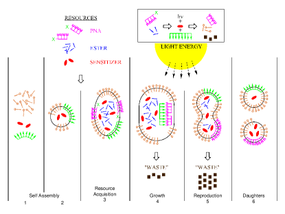
Figure 1: Schematic of the life cycle of the Los Alamos Bug: The system consists of surfactants, sensitizers, and a biopolymer that acts as a genome (1). The surfactants spontaneously self-assemble into a micellar container within which the sensitizer resides while the biopolymer sticks at the surface of the container—this forms a complete protocell (2). Resources (genomic oligomers, sensitizers and surfactant precursors in the form of esters) are added to the system and get incorporated into the container (3). The existing information carrier acts as a template for supplied oligomers to hybridize and effectively replicate the genome. Light energy is used to convert the surfactant precursor and the oligomer precursors into actual surfactant, oligomers and waste. The container grows as new surfac­tants are produced (5). Once the container reaches a critical size, it becomes unstable and divides into two daughter cells. This completes the life cycle of the protocell (6).

In the Los Alamos bug, the container is built of amphiphilic surfactants. Due to a their interaction with water, the surfactants spontaneously self-assemble into micelles with the hydrophobic end of the surfactant molecules in the interior of the micelles and their hydrophilic ends in contact with the surrounding water. The interactions between the micelle and the other components of the Los Alamos bug, namely the photosensitizer, the genome, and the container precursors, allow the micelles to host these other components.

The genomic biopolymer (possibly decorated with hydrophobic anchors) is also an amphiphile and due to the specific nature of its interactions with water and the micelle, it will tend to reside at the surface of the micelle (see figure 1.2). The sensitizer is a hydrophobic molecule and will therefore reside in the interior of the micelle. Once self-assembled, the protocell aggregate is “fed” with precursor molecules for the surfactants (oily esters), sensitizers and genomic precursor oligomers. As surfactant precursors are hydrophobic they will agglomerate inside the proto-organism and form a hydrophobic core (figure 1.3). Light energy is used by the metabolism to transform precursors into new building blocks (surfactants and oligomers) of the protocell. The genomic oligomers that are complementary with particular stretches of the template strand will hybridize with it (figure 1.4). The fully hybridized template/oligomers complex, which now only has hydrophobic elements exposed, will move into the interior of the container where polymerization of the oligomers occurs followed at some later time by a random dissociation of the fully polymerized double-stranded genome into two single-stranded templates that move back to the surface. This process could also be enhanced by a gentle temperature cycle near the gene duplex melting point.

As surfactant precursors are digested, the core volume of the protocell decreases while, at the same time, new surfactants are produced. The resulting change in the surface to volume ratio causes the micelle to become unstable (figure 1.5), until it finally splits into two daughter cells (figure 1.6). Assuming that components of the growing parent micelle are appropriately distributed upon division, the two daughter cells will be replicates of the original organism, thus completing the protocell cycle.

In the above setup, the container, genome and metabolism are coupled in various ways. Obviously, both the replication of the container and replication of the genome depend on a functioning metabolism, as the latter provides building blocks for aggregate growth and reproduction. In addition to that, the container also has a catalytic influence on the replication of both the metabolic elements and the genome: the micellar structure provides a compartment which brings precursors, sensitizers and nucleic acids in close vicinity, thereby increasing local concentrations and thus metabolic turnover. Furthermore, the micellar interface catalyzes the hybridization of the informational polymer with its complementary oligomer. Once the hybridized complex enters the “water-poor/free” interior of a micelle, the thermodynamics should change sufficiently to allow a dehydration reaction to occur whereby the oligomers become polymerized. Alternatively the water-lipid interface could either itself act as a ligation catalyst or the addition of simple amphiphilic catalysts could facilitate the gene polymerization process. Last, but not least, the nucleic acid catalyzes the metabolism, which otherwise is extremely slow. A summary of the subsystem coupling is shown in Fig. 2.

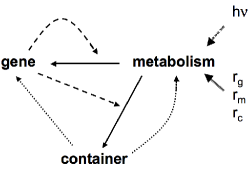
Figure 2: Functional coupling between container, metabolism and genome. Note how the gene catalyses (dashed arrows) the metabolic production (solid arrows) of both gene and container building blocks. The container ensures a high local concentrations (proximity) and facilitates thermodynamic reaction conditions (dotted arrows) of both the metabolic molecules and the amphiphilic replicator polymers. The free energy is provided by light ($h\nu$) and the provided resources are precursor lipids $r_{c}$, precursor gene oligomeres $r_{g}$, as well as sensitizers $r_{m}$.

II The model

Dissipative particle dynamics (DPD) is a mesoscale simulation method introduced by Hoogerbrugge and Koelman in 1992. The method has been improved as a result of various theoretical support, revision, and expanded capabilities [Español and Warren, 1995, Marsh, 1998, Groot and Warren, 1997], and has been applied to a number of biological systems such as membranes [Venturoli and Smit, 1999, Groot and Rabone, 2001], vesicles [Yamamoto et al., 2002, Yamamoto and Hyodo, 2003], and micelles [Groot, 2000, Yuan et al., 2002]. Also chemical reactions have been incorporated into the DPD method [Bedau et al., 2006, Buchanan et al., 2006]. In the context of protocells, DPD has recently been applied to study a self-replicating micellar system [Fellermann and Solé, 2006]. The DPD formalism used in this work is the revised version from Groot and Warren [Groot and Warren, 1997] that has become the de facto standard of DPD.

II.1 Dissipative particle dynamics

A DPD simulation consists of a set of $N$ particles located in three-dimensional continuous space with Euclidean metrics. These particles are not individual atoms but represent several water molecules or beads in a polymer chain. Each particle $i$ has a position ${\mathbf{r}}_{i}$, mass $m_{i}$ and momentum ${\mathbf{q}}_{i}$, from which one can derive its velocity ${\mathbf{v}}_{i}={\mathbf{q}}_{i}/m_{i}$. Its motion is determined by a force field ${\mathbf{F}}_{i}$ through Newton’s second law of motion:

$$\frac{d^{2}{\mathbf{r}}_{i}}{dt^{2}}(t)=\frac{1}{m_{i}}{\mathbf{F}}_{i}\left(\mathbf{r}_{i}(t)\right)$$ (1)

The force acting on particle $i$ can be decomposed into pair-wise interactions, which respectively are the sum of three different components—a conservative, a dissipative and a random one:

$$\mathbf{F}_{i}=\sum_{j\not=i}\mathbf{F}_{ij}=\sum_{j\not=i}\left(\mathbf{F}_{ij}^{C}+\mathbf{F}_{ij}^{D}+\mathbf{F}_{ij}^{R}\right)\mathbf{,}$$ (2)

where $\mathbf{F}^{C}$, $\mathbf{F}^{D}$ and $\mathbf{F}^{R}$ are defined by

$$\mathbf{F}_{ij}^{C} = -\boldsymbol{\nabla}\phi_{ij}$$ (3)

$$\mathbf{F}_{ij}^{D} = -\eta\omega^{D}(r_{ij})\left(\mathbf{n}_{ij}\cdot\mathbf{v}_{ij}\right)\mathbf{n}_{ij}$$ (4)

$$\mathbf{F}_{ij}^{R} = \sigma\omega^{R}(r_{ij})\xi_{ij}\mathbf{n}_{ij}$$ (5)

For each particle pair $(i,j)\>$ $\mathbf{r}_{ij}=\mathbf{r}_{i}-\mathbf{r}_{j}$ is the relative position, $r_{ij}=\left|\mathbf{r}_{ij}\right|$ the center-to-center distance, and $\mathbf{v}_{ij}=\mathbf{v}_{i}-\mathbf{v}_{j}$ the relative velocity. We denote with $\mathbf{n}_{ij}=\mathbf{r}_{ij}/r_{ij}$ the (unit) direction between the two particles. A detailed discussion of the different forces $\mathbf{F}_{ij}^{X}$ now follows:

The conservative force ${\mathbf{F}}_{ij}^{C}$ is expressed in the usual way as the negative gradient of a potential $\phi_{ij}=V_{ij}=V(r_{ij})$. In most DPD simulations, a pure repulsive soft core potential of the form

$$V_{ij}(r)=\left\{\begin{array}[]{cl}\frac{a_{ij}}{2}(r-r_{c})^{2}&\mbox{ if }r<r_{c}\\ 0&\mbox{ otherwise}\end{array}\right.$$ (6)

is used for all particle interactions. $a_{ij}$ and $r_{c}$ are constants that define the strength and range of the particle interaction. The magnitude of the resulting force decreases linearly from $\left|\mathbf{F}_{ij}^{C}(0)\right|=a_{ij}$ to $\left|\mathbf{F}_{ij}^{C}(r_{c})\right|=0$. The $a_{ij}$’s depend on the type of interacting particles—and are therefore the appropriate location to parameterize the model. In addition, different particles pairs could be given different values of $r_{c}$ if one wants to effectively give particles different radii. However, in the current work, we choose $r_{c}=1$ for all bead interactions, which is the standard in almost all DPD simulations.

For the study of information polymers and amphiphiles, individual DPD beads can be covalently bonded. A bond between bead $i$ and bead $j$ is formalized by an additional harmonic potential

$$V_{ij}^{s}(r)=\left\{\begin{array}[]{ll}\frac{b}{2}\left(r-r_{b}\right)^{2}&\mbox{ if $(i,j)$ are bonded}\\ 0&\mbox{ otherwise}\end{array}\right.$$ (7)

with bond strength $b$ and range $r_{b}$. In addition to that, we introduce a bending potential to stiffen longer polymer strands: In a chain $i-j-k$ of interconnected polymer beads, the angle $\theta_{j}$ formed by the two bonds of the central bead $j$ induces an additional harmonic potential

$$V_{ijk}^{\theta}(\mathbf{\theta}_{j})=\frac{\mbox{\scriptsize 1}}{\mbox{\scriptsize 2}}c_{ijk}\left(\theta_{j}-\theta_{eq}\right)^{2}\mbox{ ,}$$ (8)

where $\theta_{eq}$ is the equilibrium angle and $c_{ijk}$ denotes the strength of the bending potential.

The dissipative force ${\mathbf{F}}_{ij}^{D}$ is a function of the relative velocity of the two particles. It models the viscous damping of the fluid. The friction coefficient $\eta$ in eq. (4) scales the strength of this force and $\omega^{D}$ is a distance weighting function not determined by the general formalism.

The random force, ${\mathbf{F}}_{ij}^{R}$ accounts for thermal effects. It is scaled by a strength parameter $\sigma$ and a second weighting function $\omega^{R}$. $\xi_{ij}$ is a Gaussian distributed random variable with $\left<\xi_{ij}(t)\right>=0$, $\left<\xi_{ij}(t)\xi_{kl}(t^{\prime})\right>=(\delta_{ik}\delta_{jl}+\delta_{il}\delta_{jk})\delta(t-t^{\prime})$ and $\xi_{ij}=\xi_{ji}$.

In order to reproduce the right thermodynamic behavior, the DPD formalism must satisfy the fluctuation dissipation theorem. As a consequence, the equilibrium state will obey Maxwell-Boltzmann statistics and therefore allows the derivation of thermodynamic properties. As shown by Español and Warren [Español and Warren, 1995], DPD satisfies the fluctuation dissipation theorem if and only if the weighting functions $\omega^{D}$ and $\omega^{R}$ obey the relation

$$\omega^{D}=(\omega^{R})^{2}\mbox{.}$$ (9)

In agreement with the DPD standard, we set

$$\omega^{D}(r)=(\omega^{R}(r))^{2}=\left[2(1-\frac{r}{r_{c}})\right]^{2}\mbox{.}$$ (10)

If relation (9) is fulfilled, $\mathbf{F}_{ij}^{D}+\mathbf{F}_{ij}^{R}$ acts like a thermostat to regulate the temperature of the system and the equilibrium temperature $k_{b}T$ is given by

$$k_{b}T=\frac{\sigma^{2}}{2\eta}\mbox{.}$$ (11)

where $k_{b}$ denotes the Boltzmann constant. In molecular dynamics simulations, a variety of thermostats have been explored, but only the DPD-thermostat is guaranteed to conserve linear and angular momenta of the particles and thus flow properties of the fluid (because all involved forces are central: $\mathbf{F}_{ij}=-\mathbf{F}_{ji}$). It is therefore the only thermostat that allows the study of transport processes [Trofimov, 2003].

In agreement with the DPD standard, we use $r_{c}$ and $k_{b}T$ as our units of length and energy. All particles have unit mass $m_{i}=1$. From equation (1) we can derive the unit of time as $\tau=r_{c}\sqrt{m/{k_{b}T}}$. We will give an estimate of the order of magnitude of the physical length in section III.

II.2 Incorporation of chemical reactions

We extended the DPD formalism to account for chemical reactions. The way that chemical reactions are implemented in our model is taken from Ono [2001], where Brownian Dynamics is extended with the same algorithm.

Chemical reactions in our system occur between two reactants and fall into two different classes:

$$\mbox{transformation: }\mathbf{X} \longrightarrow \mathbf{Y}$$

$$\mbox{polymerization: }\mathbf{X}+\mathbf{Y} \longrightarrow \mathbf{XY}$$

Each reaction has a given rate for spontaneous occurrence $k_{s}$.

The spontaneous reaction rate can be enhanced by the presence of nearby catalysts. The catalytic effect decreases linearly with increasing distance to the reactant up to a cutoff distance $r_{cat}$ beyond which it is zero. For simplicity, the effect of several catalysts is modeled as a superposition. Thus, the overall reaction rate is given as

$$k=k_{s}+\sum_{\mathbf{C}}f_{cat}(r_{\mathbf{C}})$$ (12)

with

$$f_{cat}=\left\{\begin{array}[]{cl}k_{cat}\left(1-\frac{r_{\mathbf{C}}}{r_{cat}}\right)&\mbox{ if }r_{\mathbf{C}}<r_{cat}\\ 0&\mbox{else}\end{array}\right.$$ (13)

In these equations, the sum runs over all catalyst beads, with $r_{\mathbf{C}}$ denoting the distance to the first reactant, $r_{cat}$ the maximal catalytic range, and $k_{cat}$ is the catalytic rate. Polymerization has the further restriction that the distance between the reactants must be less than a maximal reaction range $R$. To deduce probabilities from the reaction rates, we used an agent-based like algorithm that is given in appendix A.

If a reaction occurs, we change the particle types of the reactants from $\mathbf{X}$ to $\mathbf{Y}$ and/or establish or remove a bond between the reactants, depending on the type of reaction. Particle positions and momenta are conserved.

We also introduced particle exchange into the model to mimic the supply of chemicals into the system, which drive it out of its equilibrium. Within a given region, particles of a certain class can be exchanged with a given probability to drive certain processes. Note that total particle number is kept constant. Likewise in chemical reactions, we conserve positions and momenta when exchanging particles.

II.3 Components of the minimal protocell model

We model the protocell with the following components: water, surfactant precursor, surfactant, sensitizer, information templates, and information oligomers and their precursors. Water ($\mathbf{W}$) and sensitizer ($\mathbf{Z}$) are single DPD particles. Surfactants are modeled as amphiphilic dimers: one hydrophilic head ($\mathbf{H}$) and one hydrophobic tail particle ($\mathbf{T}$) connected by a covalent bond. Precursor surfactants are dimers of two hydrophobic particles ($\mathbf{T}-\mathbf{T}$). Interaction parameters (as multiples of $k_{b}T$) for the water and amphiphiles have been taken from Groot [2000] (where surfactants are modeled as dimers as well):

$a_{ij}$	$\mathbf{W}$	$\mathbf{H}$	$\mathbf{T}$
$\mathbf{W}$	25	15	80
$\mathbf{H}$	15	35	80
$\mathbf{T}$	80	80	15

Bond parameters are $b=150k_{b}T$ and $r_{b}=0.5r_{c}$. These parameter values were originally used to analyze polymer surfactant interactions. Later, the phase diagram for varying surfactant concentrations was analyzed [Yuan et al., 2002].

In order to keep the number of different parameters as low as possible, we express further interactions with the same parameters as the ones above: sensitizer beads are hydrophobic. Thus, their interaction parameters are equal to those for surfactant tails: $a_{\mathbf{Z}j}=a_{\mathbf{T}j}$.

Genes

The gene is modeled as a strand of covalently bound monomers ($\mathbf{A}$ and $\mathbf{B}$) with hydrophobic anchors ($\mathbf{T}$) attached to it. We assume the gene is similar to a peptide nucleic acid (PNA) decorated with lipophilic side chains to the backbone. The reason why we are utilizing PNA and not DNA or RNA is because we want to have a non-charged backbone for the gene molecule to enhance its lipophilic properties. For details, see Rasmussen et al. [2003]. We note that the use of PNA decorated with lipophilic side chains in conjunction with an amphiphilic surface layer will cause the genetic material to have a behavior that is quite different from that of DNA or RNA in water. In particular, it is not at all clear that the two complementary macromolecules locally will lie in a common plane when hybridized with each other. Thus we investigated a number of possible different orientations.

By numbering the monomers within each strand, we introduce an orientation of the molecule that mimics the orientation of the actual peptide bond given by its C- and N-termini. This allows us to define the following vectors for each gene monomer bead: $\mathbf{u}_{i}$ is a unit vector pointing from the previous monomer towards the current one. For the first monomer in the strand $\mathbf{u}_{i}=0$. Likewise, $\mathbf{v}_{i}$ is a unit vector pointing towards the next monomer in the strand (or $0$ for the last monomer). $\mathbf{z}_{i}$ is a unit vector pointing from the actual monomer towards its anchor bead. To obtain the association of PNA to the micellar surface, the molecule is modeled as interconnected amphiphiles. For the hydrophobic anchors, we use the same bead type $\mathbf{T}$ as used for the surfactants and precursors, while nucleotide beads share the interaction parameters of the hydrophiles: $a_{\mathbf{A}j}=a_{\mathbf{B}j}=a_{\mathbf{H}j}$. We need to introduce additional interactions that describe the affinity of complementary gene monomers. Due to the rather complex combination of hydrogen bond formation and cooperative and $\pi$ stacking between real gene monomers, we cannot expect the complementary monomer bead forces to be as simple as the bead-bead interactions introduced in the former section. We now implement and test several alternative representations of such base affinities as discussed below.

undirected attraction:

The obvious extension of $\mathbf{F}^{C}_{ij}$ to include attractive interactions is a combination of attractive and repulsive components. Thus, in the first representation, we replace $\mathbf{F}^{C}_{\mathbf{A}\mathbf{B}}(\mathbf{r})$ by the stepwise linear function

$$\mathbf{F}^{C_{1}}_{\mathbf{A}\mathbf{B}}(\mathbf{r})=\mathbf{F}^{C}_{\mathbf{A}\mathbf{B}}(\mathbf{r})+\left\{\begin{array}[]{cl}a_{2}\left(r_{c_{2}}-r\right)\mathbf{n}&\mbox{ if }r<r_{c_{2}}\\ 0&\mbox{ else}\end{array}\right.$$ (14)

with $r_{c_{2}}>r_{c}$ and $a_{2}<0$. Different attraction strengths $a_{2}$ will be used and compared in later computer simulations (section III.4.1). To compensate strong attractions for small values of $r$, we will vary the repulsion strength $a_{1}=a_{\mathbf{AB}}$ accordingly. Note that another generalization of $\mathbf{F}^{C_{1}}_{\mathbf{A}\mathbf{B}}$ compared to $\mathbf{F}^{C}_{\mathbf{AB}}$ is the change in the interaction range which, in addition to the standard $r_{c}$ dependence, now also depends on the actual pair $(\mathbf{A},\mathbf{B})$ through $r_{c_{2}}$.

directed “radial” attraction:

In the real gene system, hybridization is partly due to the formation of H-bonds between the complementary nucleotides. H-bonds share features with covalent bonds, which are better characterized by directed rather than radial interactions. Hence, in the second representation, we introduce directed attraction parallel to the $\mathbf{A}-\mathbf{T}$ and $\mathbf{B}-\mathbf{T}$ axes, respectively. Here, we replace $\mathbf{F}^{C}_{\mathbf{A}\mathbf{B}}$ by

$$\mathbf{F}^{C_{2}}_{\mathbf{A}\mathbf{B}}(\mathbf{r})=\mathbf{F}^{C}_{\mathbf{A}\mathbf{B}}(\mathbf{r})\>+\>\left\{\begin{array}[]{cl}a_{2}(r_{c_{2}}-r)\left(\mathbf{z}\cdot\mathbf{r}\right)\mathbf{n}&\mbox{ if }r<r_{c_{2}}\\ 0&\mbox{ else}\end{array}\right.$$ (15)

with the above definitions for $\mathbf{r}$, $\mathbf{z}$, and $\mathbf{n}$. Again, different attraction coefficients $a_{2}$ will be compared in the later simulations. The value $a_{1}=a_{\mathbf{AB}}$, on the other hand, can be held fixed because the attraction vanishes when $r$ approaches 0. We set $a_{1}=35k_{b}T=a_{\mathbf{AA}}=a_{\mathbf{BB}}$ We call this interaction “radial”, because the strongest attraction will be radial towards the center of the micelle, once the PNA strand is attached to the surface of the micelle.

directed “tangential” attraction:

The third representation is similar to the second, except that attraction is now perpendicular to the backbone and to the $\mathbf{AT}$ (or $\mathbf{BT}$) axis. The force is attractive towards one side of the PNA and repulsive towards the other—hence, it is the only implementation that catches the directionality of the molecule:

$$\mathbf{F}^{C_{3}}_{\mathbf{AB}}(\mathbf{r})=\mathbf{F}^{C}_{\mathbf{AB}}(\mathbf{r})+\left\{\begin{array}[]{cl}a_{2}(r_{c_{2}}-r)\left(\frac{\mathbf{(}u+\mathbf{v})\times\mathbf{z}}{\left|\mathbf{(}u+\mathbf{v})\times\mathbf{z}\right|}\cdot\mathbf{r}\right)\mathbf{n}&\mbox{ if }r<r_{c_{2}}\\ 0&\mbox{ else}\end{array}\right.$$ (16)

This force is expected to be strongest tangential to the surface of the micelle. As in the last case, we will vary $a_{2}$, but keep $a_{1}$ fixed at a value of $35k_{b}T$.

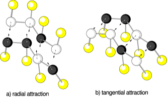
Figure 3: Hybridization complexes for radial (a) and tangential (b) attraction between complementary bases. Bases are shown as black and white beads, hydrophobic anchors in yellow. Arrows denote the direction of strongest attraction.

Covalent bonds within PNA strands have a bond strength of $b=150k_{b}T$ with an ideal bond length $r_{b}=0.5r_{c}$ for bonds between nucleotides and anchors, and $r_{b}=0.75r_{c}$ for bonds between the nucleotides themselves. In addition, we introduce stiffness (eq. 8) within the PNA strand: angles of interconnected strands prefer to be stretched out ($\theta_{0}=180^{o}$, $c_{ijk}=10k_{b}T$). With the stiffness we model folding restrictions of the peptide bond, as well as $\pi$-$\pi$ electron stacking of nearby nucleotides. This affects only the PNA chain, not the bonded hydrophobic anchors, as they do not experience any bending potential. Table 1 summarizes the chosen set of parameters.

$a_{ij}$	$\mathbf{W}$	$\mathbf{H}$	$\mathbf{T}$	$\mathbf{A}$	$\mathbf{B}$	$\mathbf{Z}$
$\mathbf{W}$	25	15	80	15	15	80
$\mathbf{H}$	15	35	80	35	35	80
$\mathbf{T}$	80	80	15	80	80	15
$\mathbf{A}$	15	35	80	35	(*)	80
$\mathbf{A}$	15	35	80	(*)	35	80
$\mathbf{Z}$	80	80	15	80	80	15

Table 1: Interaction strength $a_{ij}$ (as multiples of $k_{b}T$) for all bead types defined in the model. The force (*) between complementary nucleotides $\mathbf{A}$ and $\mathbf{B}$ has attractive parts and cannot be expressed by a single interaction parameter $a_{\mathbf{A}\mathbf{B}}$. Three different force fields have been considered for such interactions. See the text for details.

Reactions

For the above listed components we introduce the following chemical reactions:

First, we define a reaction that transforms the oil-like precursor surfactants into actual surfactants. In the real chemical implementation of the protocell, the precursors are fatty acid esters. The ester bond of the precursor surfactant breaks thereby producing a fatty acid—the surfactant—and some small aromatic molecule—which is considered waste. Disregarding the production of the waste, we model this reaction by the scheme

$$\mathbf{TT}+\mathbf{Z}\longrightarrow\mathbf{HT}+\mathbf{Z}$$ (17)

which reflects, that both parts of the ester are hydrophobic, while the resulting surfactant is an amphiphile. For simplicity, the spontaneous reaction rate is set to $0\tau^{-1}$. The sensitizer acts as a catalyst with a catalytic radius of $1.0r_{c}$. In our simulation, the catalytic rate of the sensitizer can be turned on ($k_{cat}=1.0\tau^{-1}$) and off ($0\tau^{-1}$) interactively by a switch. This mimics the photo-activity of the sensitizer.

Second, we introduce reactions to form covalent bonds between the terminal monomers of pairs of oligomers.

$$\mathbf{A}+\mathbf{B} \longrightarrow \mathbf{AB}$$

$$\mathbf{A}+\mathbf{A} \longrightarrow \mathbf{AA}$$ (18)

$$\mathbf{B}+\mathbf{B} \longrightarrow \mathbf{BB}$$

These syntheses are only applied to the terminal monomers in the PNA strands and involve no catalysts. The maximal range is $0.75r_{c}$, the maximal reaction rate is $k_{max}=0.1\tau^{-1}$. The actual reaction rate between monomers $i$ and $j$ further depends on the orientation of the ligating strands: we set

$$k_{ij}=\frac{1}{2}k_{max}\left(\frac{\mathbf{u}_{i}+\mathbf{v}_{i}}{2}\cdot\frac{\mathbf{u}_{j}+\mathbf{v}_{j}}{2}+1\right)$$ (19)

This formulation also prevents covalent bonds between complementary strands (which are anti-parallel, and thus, have an effective $k$ close to zero).

III Results

We use the model discussed above to study various aspects of the life cycle of the Los Alamos Bug as depicted in figure 1. In particular, our simulations address the spontaneous self-assembly of protocells (Fig. 1, frames 1&2), the incorporation of resources (frames 2&3), the metabolic growth of the protocell (frames 4&5), template reproduction, and finally fission into two daughter cells (frames 5&6). We will further analyze some of the catalytic coupling processes explained in the introduction.

All simulations are performed in three-dimensional space with periodic boundaries. We set $\sigma$ to 3 and $\eta$ to 4.5, which leads to an equilibrium temperature of $1k_{b}T$. A total bead density $\rho=3.0r_{c}^{-3}$ is used for all simulations. System size and number of iterations is noted for each individual simulation run. We integrate equation (1) numerically with the DPD variant of the leapfrog Verlet integrator discussed in Groot and Warren [1997] with $\lambda=0.5$ and a numerical step width of $\Delta t=0.04\tau$.

III.1 Self-assembly of micelles

We initialize a cubic box of size $(12.5r_{c})^{3}$ randomly with $2.9$ water beads and $0.05$ surfactant dimers per unit volume, or 5664 water beads and 98 dimers in the box. Simulations are performed for $0\tau<t<1000\tau$ with the interaction parameters summarized in Table 1 and the model parameters given in the introduction to this section. We observe the formation of spherical micelles with aggregation numbers up to about 20, with a peak around 12. This is shown in figure 4, where once the system had reached an equilibrium state, we followed its behavior. For each time step we recorded the number of aggregates of a particular aggregation number and hence the total number of surfactants in the aggregates of that size. The average of this result over the number of time steps was than histogrammed. We also observe a continuous exchange of surfactants with the bulk phase. As a result of these associations and dissociations, we find a number of free monomers and sub-micellar aggregates in the bulk phase. These observations qualitatively fit theoretical and experimental results [see e.g. Evans and Wennerström, 1999].

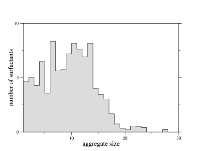
Figure 4: Micellar size distribution for a system containing $2.9$ water beads and $0.05$ surfactant dimers per unit cube. To obtain the aggregate size histograms from a system state, every two surfactants whose $\mathbf{T}$-beads are separated by less than $r_{c}$ are considered to belong to the same aggregate. 20000 systems states of an equilibrated system ($200\tau<t<1000\tau$) are averaged in the shown distribution.

Although we do not intend to model specific chemicals, we can roughly estimate the order of magnitude for the physical length scale of our simulation, using a procedure proposed by Groot and Rabone [2001]. Our calculation is based on sodium alkanesulfates as these are well studied surfactants with properties similar to the fatty acids used in the real chemical implementation. Table 2 lists the critical micelle concentration (CMC), i.e. the minimal concentration at which micelles spontaneously form. The table also gives the mean aggregation number and the volume of these molecules.

surfactant	CMC	aggregation	surfactant vol.	$N_{m}$	$r_{c}$	surfactant conc.	predicted
	in mol/l	number	in $\mbox{\AA}^{3}$		in Å	in mol/l	micellization ratio
$NaC_{6}H_{13}SO_{4}$	$0.42$	$17\pm 6$	278	4.625	7.467	0.201	$1\cdot 10^{-5}$
$NaC_{7}H_{15}SO_{4}$	$0.22$	$22\pm 10$	305	5.075	7.701	0.183	$2.5\cdot 10^{-3}$
$NaC_{8}H_{17}SO_{4}$	$0.13$	$27$	332	5.525	7.923	0.168	0.2
$NaC_{9}H_{19}SO_{4}$	$6.0\cdot 10^{-2}$	$33$	359	5.975	8.132	0.156	0.6
$NaC_{11}H_{23}SO_{4}$	$1.6\cdot 10^{-2}$	$52$	413	6.875	8.521	0.135	0.935
$NaC_{12}H_{25}SO_{4}$	$8.2\cdot 10^{-3}$	$64\pm 13$	440	7.325	8.703	0.127	1
$NaC_{14}H_{29}SO_{4}$	$2.1\cdot 10^{-3}$	$80\pm 16.5$	494	8.225	9.046	0.113	1

Table 2: Data for sodium alkanesulfate surfactants with varying tail length. For each surfactant, CMC and mean aggregation number are listed from Aniansson et al. [1976]. The molecular volume is estimated from the number $n$ of carbon atoms using the formula $V=27(n+1)\mbox{\AA}^{3}$ [Evans and Wennerström, 1999] plus a constant $88.51\mbox{\AA}^{3}$ for the sulfate group (whose value is derived from the molecular mass ($98.08g/mol$) and density ($1.84g/cm^{3}$) of sulfuric acid). The coarse graining parameter $N_{m}$, the physical length scale $r_{c}$, and the total surfactant concentration are the interpretation of model parameters in case that the model dimer represents the respective surfactant. Finally, the fraction of micellized surfactant is the prediction of the closed association model for the respective surfactant and the calculated concentration [Evans and Wennerström, 1999].

Under the simplifying assumption that all DPD beads have equal effective volume, we can derive the molecular volume of a single DPD bead and – knowing the molecular volume of water ($V_{\text{H${}_{2}$O}}=30\mbox{\AA}^{3}$) – we get the so-called coarse graining parameter

$$N_{m}=\frac{\frac{1}{2}V_{\text{surf}}}{V_{\text{H${}_{2}$O}}}$$ (20)

that tells us, how many water molecules are represented by a single DPD bead. The average number of DPD water beads per unit cube is $\rho$, each one of them representing $N_{m}$ molecules. Therefore, the physical length scale $r_{c}$ resolves to

$$r_{c}\equiv(\rho N_{m}V_{\text{H${}_{2}$O}})^{1/3}\mbox{.}$$ (21)

We will work with solutions that are quite dilute and hence dominated by water. Noting that a liter of water has $1000/18=55.56$ moles of water in it, while a volume of $r_{c}^{3}$ has $\rho N_{m}$ molecules of water in it, we find that a concentration of 1 particle/$r_{c}^{3}$ yields a unit of concentration as

$$1r_{c}^{-3}\equiv 55.56mol/\rho N_{m}\mbox{.}$$ (22)

With these estimations, we find that the lipid concentration in the above simulation represents between $0.11$ and 0.20 $mol/l$. It is somewhat arguable to estimate the concentration of free lipids in the bulk phase, because our simulations do not yield a sharp distinction between free lipids—i.e. submicellar aggregates—and proper micelles. Assuming that the most reasonable choice for such a distinction is the first minimum in the micellar size distribution at aggregates of size 5 or less, from figure 4 we get an average of 22.9 free surfactants in the bulk phase out of 98 lipids in the total volume, i.e. 76.6% of the surfactant is micellized and the free lipid concentration lies between $0.03$ and 0.05 $mol/l$. Knowing the physical surfactant concentration, we can compare this finding to the prediction of the closed association model [Evans and Wennerström, 1999]. According to this model, surfactants are either in bulk phase ($S$) or in micelles of aggregation number $N$ ($S_{N}$). With the pseudo-chemical reaction $NS\rightleftharpoons S_{N}$ and the condition that $\left.\frac{d[S]}{d[S]_{\text{total}}}\right|_{\text{CMC}}=\left.\frac{dN[S_{N}]}{d[S]_{\text{total}}}\right|_{\text{CMC}}=0.5$, one can calculate the fraction of micellized surfactant for any total surfactant concentration $[S]_{\text{total}}=[S]+N[S_{N}]$. The respective ratio $N[S_{N}]/[S]_{\text{total}}$ is also given in table 2.

We find that our model best matches the aggregation numbers of short chain surfactants ($NaC_{6}H_{13}SO_{4}$), while our micellization ratios more closely match the predictions for the somewhat longer chains ($NaC_{9}H_{19}SO_{4}$). Although our model representation of surfactants as dimers is rather simplistic, we find a reasonable match (at least in the order of magnitude) between experiment, simulation, and theory. It should be noticed that the micellization parameters for fatty acids, which are the container surfactants of choice in the Los Alamos Bug, are qualitatively similar to the listed sodium alkanesulfate surfactant parameters, which are the most well studied surfactants in the scientific community. Given the easy availability of relevant parameters for alkanesulfate surfactant parameters and the level of coarse graining in our DPD model we can safely use these experimental data to calibrate our simulation. It is conceivable that closer matches might be found by changing interaction parameters or the representation of surfactants. We have however decided to stick to the standard parameter set in order to get comparable results to earlier DPD simulations [Groot, 2000, Yuan et al., 2002, Fellermann and Solé, 2006].

Next, we analyzed a ternary mixture of water, surfactant, and oil. In the system described above, we exchanged an additional $0.1$ water beads per unit volume by $0.05$ hydrophobic oil dimers ($\mathbf{T}-\mathbf{T}$), which represent the lipid precursors of the Los Alamos Bug. Starting from a random initial condition, the system forms loaded micelles: the precursors aggregate into a core in the interior of the individual micelles because of their high degree of hydrophobicity. This core is coated by surfactants, which shield it from water. We observe a stabilizing effect from the hydrophobic core: the rate of monomer dissociation from the aggregates decreases by a factor of 4 to 5. Dissociation of oil dimers does not happen during the simulations. Over the simulated time span ($0\tau<t<1000\tau$), these loaded micelles constantly fused to form bigger aggregates. At $t=250\tau$, the system is composed of five micelles with aggregation numbers 12, 13, 16, 24, and 32, where the aggregation number just counts the surfactants in an aggregate and not any of the precursors or other components. At $t=500\tau$ we find four micelles (with sizes 16, 24, 25, 32) and finally, for $t=1000\tau$, the system consisted of only two micelles with aggregation numbers 43 and 53. It remains unclear, whether this was the equilibrium solution, or whether the two micelles would finally fuse to form a single aggregate. It is known that any given mixture of surfactants and oil in water results in some equilibrium aggregate structure, some useful and some less useful as a protocellular container substrate, see e.g. the recent summary discussion in McCaskill et al. [2006].

In general, the addition of hydrophobic precursors allows aggregates to grow far beyond their micellar aggregation number, while at the same time, monomer dissociations from the assembly falls by a factor of four or more. This is consistent with simulation results from earlier studies of a similar surfactant-precursor-water system [Fellermann and Solé, 2006]. However, a more systematic DPD investigation is necessary to address the dynamics, stability, and size distribution issue in this context.

III.2 Self-assembly of the protocell

In this section, we study the self-assembly of protocells. We initialize a cubic box of size $(7.5r_{c})^{3}$ with 1212 water particles, 21 surfactant dimers, 4 sensitizer particles and one PNA strand that is four nucleotides in length. All other simulation parameters are as before. Using these numbers, we achieve the same overall particle density and the same surfactant concentration as in the previous section.

Starting from an arbitrary initial condition, we observe the spontaneous formation of a protocell, i.e. a micelle that is loaded with sensitizer and which has PNA attached to its surface and whose nucleotides are exposed to the aqueous phase (see figure 5). Aggregation happens within a remarkably short period: after only 10 time units, we already find complete protocells. The lipid aggregation number of this micelle is around 14 with few associations and dissociations of monomers. The slight increase in aggregation number along with a decrease of monomer dissociations is most probably due to the stabilizing effect of the additional sensitizers.

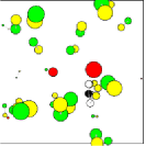
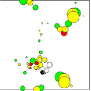
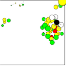
Figure 5: Self-assembly of the protocell from a random initial condition. The diagrams show the state of the system at times a) $t=0\tau$, b) $t=4\tau$, and c) $t=10\tau$. Surfactants are shown in green (head bead) and yellow (tail), the sensitizers in red, the PNA backbone in yellow and the PNA monomers in black and white.

III.3 Replication of the Container

The dynamics of a surfactant-precursor-water system similar to the one under consideration has been studied in detail in Fellermann and Solé [2006]. Considering precursor and surfactant kinetics, the formerly analyzed system differs from the one discussed here in that i) the catalytic role of sensitizers is performed by the surfactants themselves, and ii) the metabolic turnover is not regulated by turning the light on and off, but instead only follows chemical mass kinetics. Using simulations based on classical lattice gas methods, Coveney et al. in 1996 reproduced the micellar self-replication experiments of Bachmann et al. [1992]. In 1998 and 2000 Mayer and Rasmussen developed an extended lattice polymer approach for explicitly including polymers and chemical reactions similar to the current DPD approach and they were also able to reproduce the experimental findings by Luisi’s group [Bachmann et al., 1992]. The purpose of this section is to show that the reported dynamics also hold for the metabolic reaction scheme of the Los Alamos Bug.

A system of size $(10r_{c})^{3}$ is initialized with a micelle consisting of 15 surfactants and loaded with 4 sensitizer beads in its interior. Model parameters are given in the beginning of this section. In a single spherical region of radius $2r_{c}$ located away from the micelle, pairs of water particles are replaced by surfactant dimer precursors with an overall exchange rate of $\approx 2.5\times 10^{-3}$ precursors per time unit.

Because of their hydrophobic nature, the precursor molecules tend to agglomerate into oil-like droplets. The diffusion of such droplets becomes progressively slower the bigger they are. This initiates a positive feedback: the bigger the droplets, the more slowly they diffuse out of the exchange region. The slower they diffuse, the more likely they are to accumulate additional precursors before they diffuse out of the exchange volume. By varying the volume of the exchange region and/or the rate of exchange, one can set the mean size of the precursor droplets that are formed. Due to the positive feedback, the effect will not be linear with either the exchange region size or the exchange rate.

Since we do not want the non-continuous exchange events to disturb the systems dynamics too much, we restrict particle exchange to a region of $2.0r_{c}$ (3% of the total system volume). By varying the exchange rate used to introduce precursors, we find that $5.0\times 10^{-5}$ is close to the optimum for which droplets of precursor molecules are provided at a reasonable rate, yet are still small enough to diffuse at a reasonable speed. With these values, the precursor droplets consisted of 5 dimers on average. Once in the vicinity of a micelle, the droplets are immediately absorbed.

When the micelle absorbs 15 precursor molecules into its interior, we stop supplying additional precursors and trigger the catalytic activity of the sensitizer by turning on the light. During the metabolic turnover, the micelle grows in amphiphile number, while losing few, if any, amphiphiles due to the stabilizing effect of the remaining precursors as was discussed previously. It responds to the changing surfactant to precursor ratio by changing its shape from spherical to rod-like. The elongation continues until nearly all the precursors are metabolized. At some moment, the elongated aggregate becomes unstable and divides into two daughter cells (see figure 6). With the parameters used, overall precursor turnover and fission takes place in approximately 20 time units (i.e., 500 time steps).

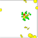
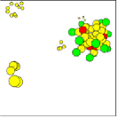
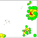
Figure 6: Replication dynamics of the container: precursors are fed into the system far from the micelle at the (periodically reflected) edge of the system space. They form droplets in the aqueous phase, which are absorbed by the protocells as a whole. Protocells grow by incorporation of precursors. After a critical amount of precursor is transformed into surfactant, the assembly loses its stability and splits in two daughter cells (right frame).

We compared the above findings to simulations of an unregulated system, where the precursor supply and catalytic rate are not triggered, but instead held constant over the whole simulated time span. The objective behind this simulation was to find whether the system might feature inherent self-regulation: as the precursor forms droplets in the bulk phase, their incorporation into the micelle occurs in spurts rather than continuously. If the introduction rate of precursors into the system is locally fast enough to allow larger droplets to form (especially due to the positive feedback effect), a larger number of precursors can simultaneously enter the protocell. Then if the metabolic turnover rate is sufficiently fast, the turnover of the large number of precursors might be sufficient to trigger container division rather than having a slow but continual loss of newly formed amphiphiles.

To investigate this possibility, we performed simulation runs for a system of size $(10r_{c})^{3}$ initialized with a micelle of 15 surfactants and 4 sensitizer beads. Other model parameters are the same as given in the beginning of this section. Precursors were supplied by the same mechanism and rate as before. We observed the incorporation of droplets between 3 and 9 precursor dimers in size. As the transformation of precursors happened significantly faster than the precursor supply, nearly each droplet was transformed separately. When only few precursors were absorbed at once (i.e. a small droplet), the micelle responded by rejecting several surfactants into the bulk phase. Such loose surfactants then formed sub-micellar aggregates or attached to precursor droplets when present. However, when the incorporated droplet was big enough, the outcome of the metabolic turnover was a proper cell division. A micelle that consisted of 15 surfactants and 4 sensitizers, for example, split in two after the absorption and turnover of 8 precursors. The fission products were two micelles, one with 14 surfactants and 3 sensitizers and the other with 9 surfactants and 1 sensitizer.

This result suggests that the explicit regulation of the metabolic turnover by light bursts might not be necessary to obtain the replication cycle of the container as a similar regulation can be obtained by a careful regulation of the provided precursor droplet sizes. Light control might, however, still serve as a convenient mechanism to synchronize container and genome replication if they occur on separate time scales.

III.4 Replication of the genome

In our experience, the most difficult component of the protocell to model with DPD methods is the genome and its behavior. Furthermore, the DPD hybridization process seems more illdefined than the ligation process, which is why our discussion of the replication of the genome is divided in two consecutive steps: hybridization and ligation. Please recall that hybridization denotes the alignment of short PNA oligomer sections along the template PNA strand and “hydrogen” bonding to it, while ligation—or polymerization—is the reaction that turns aligned oligomers into an actual (complementary) copy of the template.

III.4.1 Hybridization

Replication of the genome essentially depends on the stability of the hybridized complex: it can only occur if the double strands are stable for a time long enough for all the needed oligomers to diffuse to and align with the template. It should be noted that if more than 2 oligomers are involved, the joining of additional oligomers and their polymerization can occur sequentially so the unpolymerized templates need not all be simultaneously attached. As will be shown further below, once some polymerization has occurred, that section will be more stable in hybridized form. We studied the stability of the hybridization with the following simulation: A system of size $(5.5r_{c})^{3}$ was initialized with an oil layer that is meant to mimic a two phase system (single beads of type $\mathbf{T}$ are confined to lie below a plane above which the water is located). The overall particle density is $\rho=3r_{c}^{-3}$, as in the earlier experiments. in order to make the hybridization process as simple as possible. As we shall see later, aggregate surfactant dimers tend to tangle with the gene anchors, which both slows down the hybridization process and makes it less accurate. A four-monomer long PNA template was placed at the oil-water-interface with its anchors pointing down toward the oil and its bases pointing up towards the aqueous phase. A pair of 2-nucleotide long complementary oligomers was placed at a distance of $0.5r_{c}$ from this strand at a location/orientation for proper hybridization. The location/orientation was varied to match the different hybridization cases studied. In the case of directed radial attraction, this meant that all the beads of the complementary PNA molecules are outside the interface plane, with their hydrophobic anchors pointing away from the hybridization site. In contrast, in the case of tangential attraction, both the template and the oligomers span the interface region as shown in figure 7.

In the system modeled, we only had two different types of monomers ($\mathbf{A}$, $\mathbf{B}$) with $\mathbf{A}$ and $\mathbf{B}$ being complementary to each other, but not self-complementary. All different 4-mer templates excluding symmetric configurations were used (e.g. $\mathbf{AAAA}$, $\mathbf{AAAB}$, $\mathbf{AABB}$, $\mathbf{ABAB}$, and $\mathbf{ABBA}$) and for each different template only the proper complementary dimer oligomers were used. The different 4-mer configurations can differentially hinder the ability of the complementary bases to slide along the template.

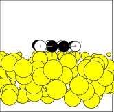
Figure 7: Initial setup of the hybridization simulations. The system is initialized with an oil-layer that mimics the oil-water interface of a two-phase system. A four-mer template and two complementary dimers are placed at the interface so that they form a hybridization complex. The association time of such hybridization complexes is measured for different PNA implementations and attraction forces.

During the simulations, the distances between all four complementary base pairs were measured at every time step. When one of these distances exceeded $1.5r_{c}$ (the maximal interaction range for complementary bases), the PNA strands were considered to be dehybridized. The time it took for the double strands to dehybridize—i.e. the association time of the hybridized complex—serves as a measure of the stability of that state. After a maximum of $t=100\tau$, simulations were truncated and the hybridization was considered to be stable.

For the three different representations of PNA hybridization (see sections II.3 Genes, cases a,b, and c), we performed simulations for all possible combinations of four bases excluding symmetrical combinations. Strengths for attractive forces were set with respect to the repulsive force parameter $a_{\mathbf{A}\mathbf{B}}$ so that complementary bases attracted each other but did not overlap by more than $0.6r_{c}$. The association times were measured using 10 to 20 runs for each combination. Results are shown in figure 8.

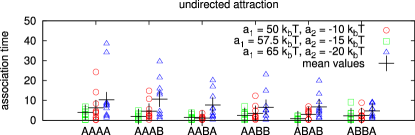
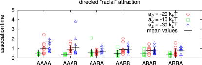
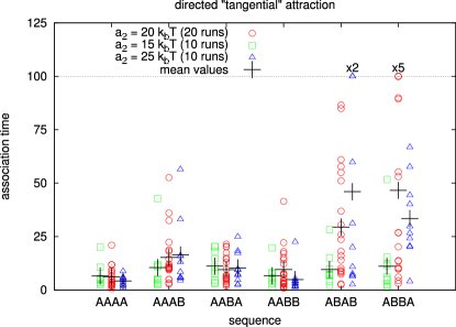
Figure 8: The association times (i.e. the time until the initially hybridized complex becomes dehybridized) for different PNA template sequences of length four using a) undirected, b) radial, and c) tangential attraction. For each implementation, three different attraction strengths are compared, as given in the legend for each figure. $a_{1}$ denotes the coefficient of the repulsive part, $a_{2}$ the coefficient of the attractive part of the interaction force. In the case of directed attraction (b and c) $a_{1}$ was set to $35k_{b}T$ independent of the respective value of $a_{2}$. In c), the plotted averages are minimal values for the actual averages, as simulations were truncated at $t=100\tau$. If runs were truncated, the multipliers above that run designate how often this was done.

undirected attraction:

In the case of undirected attraction, we found mean association times between $2.12\tau$ for $a_{1}=50k_{b}T$, $a_{2}=-10k_{b}T$, and $7.76\tau$ for $a_{1}=65k_{b}T$, $a_{2}=-20k_{b}T$. For strong attractions, association times tended to increase with the number of equal (preferably nearby) nucleotides in the template ($\mathbf{AAAA}$ is the most, while $\mathbf{ABBA}$ is the least stable sequence). However, these differences were rather small.

directed radial attraction:

For directed radial attraction, the mean association times ranged from $0.45\tau$ for $a_{2}=-10k_{b}T$ to $0.98\tau$ for $a_{2}=-30k_{b}T$ ($a_{1}=a_{\mathbf{AB}}=35k_{b}T$ for all cases) without any significant variation for different sequences. For most simulation runs, it took only a few time steps for the initial complex to dehybridize. The reason for the poor nature of the hybridization of the PNA for the radial attraction is quite obvious: due to the amphiphilic character of PNA, the strands will arrange so that nucleotides point towards water and the anchors towards oil. Thus, the attraction is directed perpendicular to the oil-water interface and into the aqueous phase where the oligomers do not want to reside. Because of the dot product in equation (15), the attraction between two PNA molecules on the interface is marginal and the association time is essentially a matter of diffusion.

directed tangential attraction:

In contrast to the other tested situations, in the case of directed tangential attraction, one can see significant differences in the association time of the initial hybridized complexes, provided the attraction is strong enough: for gene sequences with pairs of equal bases at terminal positions (e.g. $\mathbf{AAAA}$ and $\mathbf{AABB}$), hybridization is usually less stable than for sequences without equal bases at terminal positions ($\mathbf{ABBA}$ and $\mathbf{ABAB}$). The association time of sequences with only one such dimer lies between the values of the above two situations. Examination of the simulations reveal the cause of this trend: a continuous group of two or more equal monomers, one of which is a terminal position of the template allows the attached dimer to slide along the template strand without a strong penalty in potential energy, and eventually protrude beyond the end of the template. In this misaligned configuration, the dimer can easily distort from the parallel alignment, thereby reducing the overall attraction to the template, until it finally disassociates from the complex. Distinct bases at terminal positions, on the contrary, prevent this sliding along and then off of the template, thereby significantly stabilizing the hybridized state.

For the more promising PNA implementations—undirected and tangential attraction—we further measured the mean distance between complementary bases (hybridization distance) and the distance between those bases in the oligomers that are supposed to polymerize (ligation distance). We performed these measurements using the sequence $\mathbf{AAAA}$ for the undirected, and $\mathbf{ABBA}$ for the tangential attractions (interaction parameters are given in the caption of figure 9). Simulations are performed for $0\tau\leq t\leq 1000\tau$. The resulting time series are shown in figure 9.

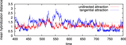
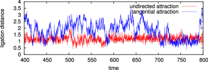
Figure 9: Mean hybridization (upper panel) and ligation distance (lower panel) for the PNA templates (and corresponding oligomers) $\mathbf{AAAA}$ using undirected attraction with $a_{1}=65k_{b}T$, $a_{2}=-20k_{b}T$ (red) and for $\mathbf{ABBA}$ using tangential attraction with $a_{1}=35k_{v}T,a_{2}=40k_{b}T$ (blue). By hybridization distance, we mean the average distance between complementary nucleotides, by ligation distance, we mean the minimal distance between two terminal nucleotides that are supposed to polymerize. The maximal values of the various distances are limited by the small size of the box.

In the case of tangential hybridization one finds two alternating domains in the hybridization distance time series: (i) when oligomers are aligned to the template, the mean hybridization distance is around $1.04r_{c}$ with only small fluctuations and an average ligation distance of $1.01r_{c}$ (e.g. $430\tau\leq t\leq 450\tau$ and $700\tau\leq t\leq 780\tau$ in figure 9). In between such periods, (ii) oligomers dissociate from the template, and diffuse over the interface, which is indicated by the large variance in hybridization distance.

Undirected attraction, in contrast, yields hybridization distances around $1.07r_{c}$ with significant continual fluctuations and a mean ligation distance of $1.158r_{c}$. One cannot observe the “locking” of the hybridized state that is apparent for the tangential attraction: although the oligomers preferably stay in the vicinity of the template, they are not forced into any particular orientation. Investigation of simulation states reveals that oligomers align along different sites of the template or even cross the template strand. Thus, although it appears from a quick look at figure 9 that the undirected attraction performs better on average, it is only during the “locked in” period that the desired reactions occur. We can therefore conclude that only the implementation of PNA using tangential attraction is able to generate a proper hybridization and base recognition approximation.

It is assumed that the PNA replication is catalyzed by the oil-water or surfactant-water interface. This is because: (i) lipophilic PNA concentrates at the oil-water interface and thus obtains a much higher local concentration there than in water; (ii) that the interface contains a lower water concentration than the bulk phase; (iii) that the interface might directly act as a catalyst for the amide bond formation; and (iv) that the PNA is more spread out (linear) when attached to the interface. To test the geometric part of this hypothesis, we also performed simulations of hybridization in pure water. We randomly initialized a box of size $(5.5r_{c})^{3}$ with water, PNA template ($\mathbf{ABBA}$) and complementary oligomers using directed tangential forces (the overall bead density was $\rho=3r_{c}^{-3}$). Simulations were performed for $0\tau\leq t\leq 1000\tau$. Hybridization and ligation distances are plotted in figure 10.

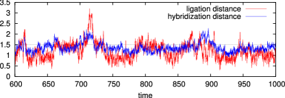
Figure 10: Hybridization and ligation distances of PNA template and complementary oligomers in water. For PNA, tangential directed attraction with $a_{2}=40k_{b}T$ has been used. The nucleotide sequence is $\mathbf{ABBA}$.

The mean hybridization distance in this scenario is $1.41r_{c}$ (which is close to the maximum radius $r_{c_{2}}$ at which attraction of complementary nucleotides still exists) with a standard deviation of $0.34r_{c}$. Moreover, there is no clear separation between hybridized and dehybridized states. In contrast to the scenario for the oil-water interface, the oligomers never completely dissociate from the template. However, the oligomers are not properly hybridized either. Instead, the template and complementary strands mainly attract each other due to the hydrophobic interactions between the tail beads of these strands rather than forces between their bases. Inspection of the simulated states shows that oligomers are seldom aligned parallel to the template. The overall structure has more resemblance to that of a micelle with geometries defined by the amphiphilic properties of the molecules, rather than a double strand defined by base affinities. The ligation distance has an average value of $1.12r_{c}$ with a standard deviation of $0.39r_{c}$. Unfortunately, this is smaller than in the previous simulations. This might result in ligation rates higher than those on the surface. However, if we decide to vary the ligation probability depending on the angle between PNA backbones, the effective ligation rate is smaller than at the oil-water interface.

Last but not least, it is notable that we cannot achieve reliable hybridization without a stiffness potential in the PNA chain. In the absence of such stiffness, complementary bases within one strand tend to bind to each other and form sharp hairpin loops even for very short strands. This effectively hinders any proper hybridization except for very few sequences that do not offer any possibility for loop formation (such as $\mathbf{AAAA}$).

III.4.2 Ligation

To study the polymerization reaction, a four-mer template strand and two complementary dimers are placed randomly on the surface of a loaded micelle (20 surfactant, 20 precursors) within a system of size $(10r_{c}^{3})$ and total density $\rho=3.0r_{c}^{-3}$. As the last section identified $\mathbf{ABBA}$ to form the most stable hybridization complex, we restrict polymerization experiments to this particular sequence using the PNA representation with tangential directed attraction (see figure 11).

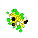
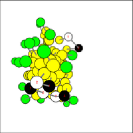
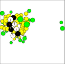
Figure 11: The three steps of template directed replication: a) Template ($\mathbf{ABBA}$) and oligomers ($\mathbf{BA}$ and $\mathbf{AB}$) diffuse over the surface of the micelle, b) oligomers form a hybridization complex with the template strand, and c) oligomers polymerize to yield a complementary copy of the template.

Of the performed simulations, 8 out of 10 generated proper template directed ligation, while the remaining 2 reactions occur spontaneously in the absence of the template strand and define the expected background reaction [Nielson, 2007]. In our simulations, one of the two spontaneous ligation results was a correct complementary copy of the template strand while the other was not. Note that in our simulation, polymerization has not been explicitly restricted to happen only between C- and N-terminals, which means that both ends can be concatenated with any other end. When ligation is template directed, 6 out of 8 runs lead to correct complementary sequences, while the other two resulted in mispairings of the form $\mathbf{BABA}$. In summary, we find that correct replication is about $50\%$ more reliable, when directed by the template. If one prohibits the ligation of equal terminal beads (C-C and N-N), the reliability of replication is expected to further increase.

The simulations reveal that it can take a surprisingly long time for the oligomers to form a ligated hybridized complex with the template. Ligation occurs after $90\tau$ in the fastest and after $674\tau$ in the slowest run. The average time is estimated as $223.2\tau$. The huge variance is due to the random walk of template and oligomers over the surface of the micelle. Compared to the oil-water interface of the previous section, oligomer motion is further slowed down by the head particles of the amphiphiles as well as the dimer structure of the aggregate building blocks.

It is worth mentioning that as expected, the hybridized complex is significantly more stable after the ligation has occured than before. None of the hybridized complexes that formed in the above simulations showed any sign of dissociation within 750 time units after ligation took place.

III.5 Full protocell division

The last elemental step in the life cycle of the Los Alamos Bug is the fission of the grown cell into two daughter cells as shown in figure 12. In addition to what was discussed in section III.3, here we studied the fission of the whole protocell after the replication of its genome, that is, a micelle loaded with some lipid precursors, sensitizers and two complementary PNA templates. The objective is to illuminate how templates and sensitizers are distributed among the daughter cells. Although not addressed by simulations in earlier sections, here the influence of the number of sensitizers is also investigated.

Proper division into two daughter cells requires the melting of the double stranded PNA resulting from genome replication, which may be achieved by a temperature cycle. In the DPD formalism, temperature translates into the interaction parameters $a_{ij}$. To study the impact of a temperature cycle on the whole system, one would need to exchange the interaction parameters between all DPD beads. For simplicity in these initial investigations, and in the absence of a rigorous calibration of our model, we chose to invoke melting by simply turning off the attractive hybridization interactions between the PNA bases.

We performed simulations of a system of size $(10r_{c})^{3}$ with an initial protocell consisting of 20 surfactants, 20 precursors, 4 to 8 sensitizers, and two PNA template strands randomly located on its surface. Otherwise, the standard parameters listed in the beginning of this section were used. Snapshots of the system are shown in Fig. 12.In all cases, metabolic turnover initiated the division of the aggregate at times of between 50 to 100 $\tau$ after the start of the simulation. Fission times were found to be longer than in the former experiments. This was because the aggregate consisted of more particles and because the template strands stabilized the rod-like aggregate that precedes protocell division. It was observed that PNA strands were preferably located along the elongated part of the aggregate, rather than at the caps. We believe that due to the stiffness parameter (eq. (8)) of the PNA strands, the aggregate tends to elongate in a direction that is parallel to the PNA’s long axis.

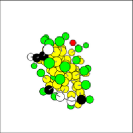
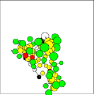
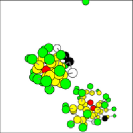
Figure 12: The division of the whole protocell completes the life cycle of the Los Alamos Bug. A mature protocell is loaded with precursor molecules, sensitizers, and two complementary PNA strands. During the metabolic turnover of precursors, the aggregate elongates and divides. Both PNA strands and sensitizer molecules tend to distribute evenly among the daughter cells, when only few sensitizers are present.

Using only 4 sensitizers, the distribution of sensitizers and PNA among the daughter cells was rather diverse: in one out of 10 runs, all sensitizers and templates remained in one of the fission products, while the other consisted of only 11 surfactants. In 7 of the runs the partition was nearly even: both sensitizers and templates were equally distributed among the two daughter cells, which differed in aggregation number by at most 3 surfactants. Last but not least, we also observed two runs where the other components were distributed equally, but one of the daughter cells contained both template strands. We note that although it was not observed, it might be possible for a template to connect two otherwise divided aggregates by attaching to both their surfaces.

One might expect the equipartition of sensitizers is more likely when their number is increased. Our simulation results, however, showed quite the opposite: protocells loaded with 8 sensitizers instead of 4 almost always responded by rejecting an average of 11 to 12 surfactants. By doing so, the protocell was able to maintain a stable spherical shape even with an aggregate number of 27 surfactants. This is due to the collective stabilizing effect of the strongly hydrophobic core of sensitizers within the aggregate. The more sensitizers that are added, the more they will tend to stick together. The more they stick together, the less likely they will partition into different daughter cells. Thus they are better able to stabilize the amphiphilic dimers in the aggregate. For an initial protocell that holds 6 sensitizers, proper division can still be observed, but the results are less reliable than in the case of 4 sensitizers. For 6 sensitizers, equipartition of sensitizers was only achieved in one out of five simulations. The other runs lead to empty micelles or a situation where one of the daughter micelles has only one sensitizer bead. Equipartition of PNA could not be achieved for the cases with either 6 or 8 sensitizer beads.

IV Discussion

Because of the inherent simplifications of the aggregated DPD simulation technique and due to the inherent complexity of our protocell system, accurate predictions of neither the detailed kinetic nor thermodynamic properties could be expected. However, insights into generic issues and likely system behavior could be obtained by the illumination of the systemic properties of the proposed protocell design. In particular we were able to see how the global behavior emerges from the simple and well-defined properties of the underlying molecular ingredients. Interpolation between several simulation methods combined with experimental data is necessary to obtain predictive understanding of this protocellular system. Investigations based on quantum mechanics, molecular dynamics, reaction kinetics, combined with these and other DPD studies, hopefully can address the quantitative prediction issues in a more complete manner [PAs & PACE, 2004-2008].

We found that the micellar kinetics that underlie the container replication are highly affected by hydrophobic molecules present in the solution. In the design of the Los Alamos Bug, these hydrophobic molecules can be the metabolic precursors and sensitizers. As these molecules are incorporated into the protocell, they form a core that stabilizes the aggregates. Such loaded micelles have a larger aggregation number than micelles in a pure surfactant-water system, and the surfactant exchange with the bulk phase is strongly decreased. The simulations thus suggest that a 3-component (ternary) surfactant-oil-water system is more suitable for yielding a suitable container than a two-component system based on surfactant and water only.

We also observed that protocells grow in spurts rather than continuously, even with a continuous supply of resource molecules. This is because the oil-like precursor molecules form droplets before they are absorbed by the aggregates. Furthermore, due to slower diffusion of larger objects, once the droplets start to form, volume-wise they will tend to grow ever more rapidly the larger they become prior to being absorbed. The spurt-like support of resources might be sufficient to initiate the division process of the aggregate if these droplets have the appropriate size. If so, the system would be self-regulated and no further triggering of the metabolism as with an external light switch would be necessary. Whether or not this self-regulation enables a reliable replication of the whole organism also depends on a number of other factors such as the rate of precursor supply compared to the replication rate of the genome. Further simulation investigations will be necessary to identify whether the metabolic self-regulation is sufficient when the precursor supply rate is not carefully balanced.

Our representations of the biopolymer that stores genomic information can be considered to be the crudest feature of the model. None of the implementations relate in detail to the actual physicochemical traits of the real PNA molecule. The behavior of the PNA molecule with hydrophobic side chains in our protocell is also found to be quite different from that seen for DNA or RNA in water. Unlike DNA where hybridized base pairs are radially opposite, in our PNA the hybridized bases are more likely to line up side by side in our attempts to model them. Furthermore, we have not been able to achieve an appropriate modeling of the balance between the hydrogen bond formation and the $\pi$ stacking between the bases in large part due to the hydrophobic and amphiphilic elements involved. More work and new ideas are needed here. However, we believe that the most fundamental properties of the biopolymer used—a PNA strand decorated with hydrophobic anchors that is able to hybridize with another PNA strand via H-bonds—is captured, at least in a qualitative manner. Against the background of this caveat, two findings are of particular interest: the simulations reveal that even our simple template representations are sufficient to introduce an impact on the stability of the hybridization complex. In other words, it is observed how a molecular fitness function emerges from very few assumptions about the underlying molecular implementation. Furthermore, this fitness function is not a simple superposition of the individual monomer properties, but rather depends on the sequence of nucleotides in the genome.

Equipartition of the components among the daughter cells after the division was achieved only when a few hydrophobic sensitizers are present in the protocell. Above a minimal number of sensitizers, equipartition becomes less probable as the number of sensitizers is further increased. This counter-intuitive finding is connected to the fact that sensitizers, like precursors, form a hydrophobic core in the interior of the micelle, thereby increasing the allowed size of stable aggregates, in addition to stabilizing them overall. Since the stability of the core itself increases with its size, once large enough, it becomes nearly impossible for the core and therefore the protocell as a whole to divide. Instead, the instability caused by the excess surfactants is addressed by rejecting excess individual surfactants one at a time. The results suggest that the volume of the sensitizer molecules most likely will affect the fission dynamics when a certain threshold is reached.

Many open questions about systemic issues are still left unanswered by these initial investigations. The main open issues include: (i) What is the effect of heating the whole system in order to de-hybridize the gene templates? Obviously, the lipid aggregate has to be more heat tolerant than the gene duplex. (ii) What is the effect of defining the gene duplex as the photo-catalyst as in the originally proposed protocell design [Rasmussen et al., 2003]? In our simulations, the sensitizer has been assumed to do the photo-fragmentation without any genetic catalysis. Also, what is the effect of having the sensitizer as a separate molecule (as reported here) versus covalently linking it to the gene, e.g. as one of the lipophilic anchors? (iii) What is the effect on the overall protocell replication if both the gene precursors (oligomers) and the lipid precursors are supplied to the solution and have to diffuse to the protocell? In such a case, will we see the coordinated gene and container growth based on reaction kinetics predicted by Rocheleau et al. [2006]? As gene replication is necessary before container division for two viable daughters, can that be ensured in other ways than through a sequential resource supply? (iv) What new issues arise when the protocell goes through more than one generation of its life cycle, e.g. due to complementary resource sequence supplies?

Subsequent work in this area must also relate the DPD simulation implementation in this publication and its dynamics with corresponding molecular dynamics simulations [Weronski et al., 2006] and reaction kinetics studies [Knutson et al., 2006] as well as experimental findings as they arise.

V Conclusion

The overall replication dynamics that constitute the life cycle of the Los Alamos Bug was implemented using DPD simulations. In particular, we investigated the dynamics of container, metabolic complex, and genome subsystems, as well as the mutual interaction between these individual components. Component diffusion, self-assembly, precursor incorporation, metabolic turnover, template directed replication of the gene, and finally the protocellular division were studied in various simulations. The main systemic finds are: (a) Metabolic growth orchestration can be coordinated by a switchable light source and/or by a continuous light source together with regulation of the size and frequency of the oily precursor package injection, which was not anticipated. (b) As anticipated, there is a tradeoff between the lipophilic strength of the genetic backbone that makes it stick to the aggregate and its ability to easily hybridize with a complementary string. (c) As anticipated, for PNA with hydrophobic side chains, three dimensional structure formation that can potentially inhibit appropriate hybridization is more likely in water than at an oil-water or lipid-water interface, although this is in part also dependent on the type pf hybridization attraction. (d) Gene replication is easier at the surface of a micelle with a substantial oil core than for a micelle with a little or no oil core. The larger the oil core is, the easier the gene replication becomes due to the aggregate stability and the ability to have a linear template. (e) As anticipated, the stability of two full complementary gene strings is much higher than a gene template and two complementary unligated gene pieces. (f) Rather surprisingly we observe that the template directed replication rate is dependent on the monomer component sequence and not only on the monomer component composition. (g) Partition of lipids, sensitizers, and gene between daughter cells strongly depends on the size of the oil core. The smaller the oil core is, the more balanced the partition becomes, which was not anticipated.

These systemic findings are now being considered in the experimental designs being pursued as part of the Protocell Assembly (PAs) and Programmable Artificial Cell Evolution (PACE) collaborations and their validity will eventually be addressed as the experiments are executed.

Appendix A Algorithm for chemical reactions

Between every two DPD time steps, the following algorithm is applied to perform chemical reactions: For every reaction scheme, we successively check all possible pairs of reactants $A,B$, and compare their effective reaction rate $k$ to a number taken from a suitably normalized pseudo-random number generator. If the reaction rate is smaller than this value, we perform the reaction and go on to the next pair of possible reactants. However, $A$ and $B$ will not be considered again in this step. The exact algorithm—notated in the Python programming language—reads as follows:

shuffle(reaction_list)
for reaction in reaction_list :
  for A in space.particles(reaction.educt_A) :

    if reaction.is_synthesis :
      # if reaction is a synthesis, possible
      # reaction partners are particles
      # of type educt_B in the vicinity of A.
      partners = A.neighbors(
        reaction.educt_B,reaction.R
      )

    else :
      # otherwise, possible reaction partners
      # are particles of type educt_B bonded to A.
      partners = A.bonded(reaction.educt_B)

    for B in partners :
      # compute effective reaction rate
      k = reaction.k
      for C in A.neighbors(
        reaction.catalyst,reaction.r_cat
      ) :
        k += reaction.k_cat *
          (1-(A.pos-C.pos).length()/reaction.r_cat)

        if random() < dt * k :
          # perform reaction
          react(A,B,reaction)
          # and leave loop over partners
          continue

References

- Alberts et al. [2002] B. Alberts, A. Johnson, J. Lewis, M. Raff, K. Roberts, and P. Watson. Molecular Biology of the Cell. Garland Science Publishing, 2002.
- Aniansson et al. [1976] E. A. G. Aniansson, S. N. Wall, M. Almgren, H. Hoffmann, L. Kielmann, W. J. Ulbricht, R. Zana, J. Lang, and C. Tondre. Theory of the kinetics of micellar equilibria and quantitative interpretation of chemical relaxation studies of micellar solutions of ionic surfactants. J. Phys. Chem., 80:905, 1976.
- Bachmann et al. [1992] P. Bachmann, P. Luisi, and J. Lang. Autocatalytic self-replicating micelles as models for prebiotic structures. Nature, 357:57–59, 1992.
- Bedau et al. [2006] M. Bedau, A. Buchanan, G. Gozzala, M. Hanczyc, T. Maeke, J. McCaskill, I. Poli, and N. Packard. Evolutionary design of a ddpd model of ligation. In Proceedings of the 7th International Conference on Artificial Evolution EA’05, pages 201–212. Springer, 2006.
- Buchanan et al. [2006] A. Buchanan, G. Gazzola, and M. A. Bedau. Systems Self-Assembly: multidisciplinary snapshots, chapter Evolutionary Design of a Model of Self-Assembling Chemical Structures. Elsevier, 2006.
- Coveney et al. [1996] P. V. Coveney, A. N. Emerton, and B. M. Boghosian. Simulation of self-reproducing micelles using a lattice-gas automaton. J. Amer. Chem. Soc., 118:10719–10724, 1996.
- Español and Warren [1995] P. Español and P. Warren. Statistical mechanics of dissipative particle dynamics. Europhys. Lett., 30:191–196, 1995.
- Evans and Wennerström [1999] D. Evans and H. Wennerström. The Colloidal Domain - Where Physics, Chemistry, Biology, and Technology Meet. Wiley-VCH, New York, 1999.
- Fellermann and Solé [2006] H. Fellermann and R. Solé. Minimal model of self-replicating nanocells. Phil. Trans. R. Soc. Lond. B, 2006. in press.
- Ganti [2003] T. Ganti. The Principles of Life. Oxford University Press, 2003.
- Groot [2000] R. D. Groot. Mesoscopic simulation of polymer-surfactant aggregation. Langmuir, 16:7493–7502, 2000.
- Groot and Rabone [2001] R. D. Groot and K. L. Rabone. Mesoscopic simulation of cell membrane damage, morphology change and rupture by nonionic sufactants. Biophysical Journal, 81:725–736, 2001.
- Groot and Warren [1997] R. D. Groot and P. B. Warren. Dissipative particle dynamics: Bridging the gap between atomistic and mesoscale simulation. J. Chem. Phys., 107(11):4423–4435, 1997.
- Hanczyc and Szostak [2004] M. Hanczyc and J. Szostak. Replicating vesicles as models of primitive cell growth and division. Current Opinion in Chemical Biology, 8:660–664, 2004.
- Hoogerbrugge and Koelman [1992] P. Hoogerbrugge and J. Koelman. Simulating microscopic hydrodynamic phenomena with dissipative particle dynamics. Europhys. Lett., 19:155–160, 1992.
- Knutson et al. [2006] C. Knutson, G. Benkö, T. Rocheleau, F. Mouffouk, J. Maselko, A. Shreve, L. Chen, and S. Rasmussen. Metabolic photo-fragmentation kinetics for a minimal protocell. Artifical Life, 2006.
- Luisi et al. [1994] P. Luisi, P. Walde, and T. Oberholzer. Enzymatic RNA synthesis in selfreproducing vesicles: An approach to the construction of a minimal synthetic cell. Ber. Bunsenges. Phys. Chem., 98:1160–1165, 1994.
- Marsh [1998] C. Marsh. Theoretical Aspects of Dissipative Particle Dynamics. PhD thesis, Lincoln College, University of Oxford, 1998.
- Mayer and Rasmussen [1998] B. Mayer and S. Rasmussen. Self-reproduction of dynamical hierarchies in chemical systems. In Artificial Life VI Proceedings, pages 123–129. MIT Press, 1998.
- Mayer and Rasmussen [2000] B. Mayer and S. Rasmussen. Dynamics and simulation of micellular self-reproduction. Int. J. Mod. Phys. C, 11:809–826, 2000.
- McCaskill et al. [2006] J. McCaskill, N. Packard, S. Rasmussen, and M. Bedau. Evolutionary self-organization in complex fluids. Phil. Trans. R. Soc. Lond. B, 2006. in press.
- Nielson [2007] P. Nielson. Protocells: Brdiging nonliving and living mater, chapter Peptide nucleic acid (PNA) as prebiotic and abiotic genetic material. MIT Press, 2007. in press.
- Ono [2001] N. Ono. Artificial Chemistry: Computational Studies on the Emergence of Self-Reproducing Units. PhD thesis, Institute of Physics, University of Tokyo, 2001.
- PAs & PACE [2004-2008] PAs & PACE, 2004-2008. An integrated multiscale computational and experimental approach is applied in the Los Alamos National Laboratory sponsored Protocell Assembly (PAs) project and the European Commission sponsored Programmable Artificial Cell Evolution (PACE) project.
- Pohorille and Deamer [2002] A. Pohorille and D. Deamer. Artificial cells: prospects for biotechnology. Trends in Biotechnology, 20:123–128, 2002.
- Rasmussen et al. [2003] S. Rasmussen, L. Chen, M. Nilsson, and S. Abe. Bridging nonliving and living matter. Artificial Life, 9:269–316, 2003.
- Rocheleau et al. [2006] T. Rocheleau, S. Rasmussen, P. E. Nielson, M. N. Jacobi, and H. Ziock. Emergence of protocellular growth laws. Phil. Trans. R. Soc. B, 2006. in press.
- Trofimov [2003] S. Trofimov. Thermodynamic consistency in dissipative particle dynamics. PhD thesis, Technische Universiteit Eindhoven, 2003.
- Venturoli and Smit [1999] M. Venturoli and B. Smit. Simulating self-assembly of model membranes. Phys. Chem. Comm., 10, 1999.
- Weronski et al. [2006] P. Weronski, Y. Jiang, and S. Rasmussen. Molecular dynamics (MD) study of small PNA molecule in lipid-water system. J. Biophys., 2006. in press.
- Yamamoto and Hyodo [2003] S. Yamamoto and S. Hyodo. Budding and fission dynamics of two-component vesicles. J. Chem. Phys., 118(17):7937–7943, 2003.
- Yamamoto et al. [2002] S. Yamamoto, Y. Maruyama, and S. Hyodo. Dissipative particle dynamics study of spontaneous vesicle formation. J. Chem. Phys., 116(13):5842–5849, 2002.
- Yuan et al. [2002] S. Yuan, Z. Cai, and G. Xu. Dynamic simulation of aggregation in surfactant solution. Acta Chimica Sinica, 60(2):241–245, 2002.