High Lewis number combustion wavefronts: a perturbative Melnikov analysis

Abstract

The wavefronts associated with a one-dimensional combustion model with Arrhenius kinetics and no heat loss are analyzed within the high Lewis number perturbative limit. This situation, in which fuel diffusivity is small in comparison to that of heat, is appropriate for highly dense fluids. A formula for the wavespeed is established by a non-standard application of Melnikov’s method and slow manifold theory from dynamical systems, and compared to numerical results. A simple characterization of the wavespeed correction is obtained: it is proportional to the ratio between the exothermicity parameter and the Lewis number. The perturbation method developed herein is also applicable to more general coupled reaction-diffusion equations with strongly differing diffusivities. The stability of the wavefronts is also tested using a numerical Evans function method.

1 Introduction

In this article, we study the wavespeed of a combustion wavefront along a one-dimensional medium. This is a fundamental idealized problem towards understanding how flame fronts propagate, and therefore has received a considerable amount of attention. There are several (non-dimensional) parameters of importance: the Lewis number Le, the exothermicity parameter $\beta$, and the heat loss parameter $\ell$. The first of these, the Lewis number, measures the relative importance of fuel diffusivity in comparison to that of heat. The exothermicity $\beta$ is the ratio of the activation energy to the heat of reaction. The structure of the governing equations is such that an infinite Lewis number is considerably easier to deal with than allowing for fuel diffusivity. Many studies of this “solid” regime appear in the literature [36, 37, 28, 7, 5], and also the “gaseous” regime ${\mbox{Le}}\approx 1$ has been frequently studied because of a symmetry in the equations [37, 20, 7, 24, 39]. Usually, the heat loss is neglected in these “adiabatic” studies. In several of these articles [37, 36, 28] the condition $\beta\gg 1$ is essential to the wavespeed and stability analysis. The case $\beta\ll 1$ has also been studied [8], in which a perturbative method is used to model the temperature. The bifurcation structure with respect to the heat loss parameter $\ell$ is addressed in [34], which obtains a stability diagram with respect to $\ell$ and the wavespeed.

We note that the limit of small fuel diffusivity (large, but not infinite, Lewis number) has not received much attention, perhaps because of the singularity of this limit in the governing equations. Yet this limit may be argued to be particularly appropriate for very high density fluids burning at high temperatures, such as would occur, for example, in the burning of toxic wastes at supercritical temperatures [25]. Even for solids, some mass diffusivity is to be expected at very high temperatures, particularly in the reaction zone in which liquification may occur. In [27], the mass diffusivity is modeled by an Arrhenius temperature dependence, which would result in a large effective Lewis number in certain situations (such as when the [scaled] adiabatic flame temperature is small in comparison to the activation energy for mass diffusion). It is this very large Lewis number limit which we study in this article, without restricting $\beta$. We do a detailed analysis of the wavespeed of combustion waves which can be supported. We also verify the linear stability of such wavefronts using an Evans function technique.

The model we use is for a premixed fuel in one dimension, with no heat loss and with an Arrhenius law for the reaction rate. These combustion dynamics can be represented in non-dimensional form by [37, 20, 34, 5, 8, 36, 28, 24, 39]

$$\left\{\begin{array}[]{lll}\displaystyle\frac{\partial u}{\partial t}&=&\displaystyle\frac{\partial^{2}u}{\partial x^{2}}+y\,e^{-1/u}\\ \displaystyle\frac{\partial y}{\partial t}&=&\displaystyle\frac{1}{{\mbox{Le}}}\,\frac{\partial^{2}y}{\partial x^{2}}-\beta\,y\,e^{-1/u}\end{array}\right.\,.$$ (1)

Here, $u(x,t)$ is the temperature, and $y(x,t)$ the fuel concentration, at a point $x$ at time $t$. The parameters $\beta$ and Le are as described earlier. We are neglecting heat loss (had we included it, an additional term $-\ell\left(u-u_{a}\right)$ for some ambient temperature $u_{a}$ would be necessary on the right-hand side of the $u$ equation in (1)). This one-dimensional model is also applicable to combustion in cylinders [30], with $u$ and $y$ being cross-sectionally averaged quantities in this case. See also [19, 26, 6, 7] for closely related governing equations. The non-dimensionalization leading to (1) ensures that the cold boundary problem is circumvented (see [36] for a discussion). Since the Lewis number will be assumed large, set $\epsilon=1/{\mbox{Le}}$ with $0\leq\epsilon\ll 1$. This small $\epsilon$ limit clearly constitutes a singular perturbation in (1).

This article analyzes (1) as follows. In Section 2, we determine the wavespeed as a function of $\beta$ and $\epsilon$. We initially consider the situation where ${\mbox{Le}}=\infty$ (Section 2.1), since this wavespeed is relevant to our subsequent perturbative analysis for $1\ll{\mbox{Le}}<\infty$ (Sections 2.2, 2.3 and 2.4). While the infinite Lewis number situation is well-studied, we are able to empirically determine a simple exponential formula for the wavespeed as a function of $\beta$. The case $1\ll{\mbox{Le}}<\infty$ is initially examined numerically in Section 2.2, in which we obtain a method for computing the wavespeed. In the subsequent sections, we establish a theoretical estimate for the wavespeed with the help of two suitably modified tools from dynamical systems theory: a slow manifold reduction, and Melnikov’s method. In Section 2.3, we reduce the dimensionality of the problem using a slow manifold reduction argument. This enables us in Section 2.4 to utilize a non-standard adaptation of Melnikov’s method to find a theoretical estimate for the wavespeed. (This new technique is adaptable to other situations in which the wavespeed correction due to the presence of a small parameter is needed.) Our asymptotics enable the determination of a remarkably simple formula for the wavespeed, which is accurate for all $\beta$ values (and not restricted to the “usual” large $\beta$ limit). Essentially, we find that the relative wavespeed correction in going from infinite to large Lewis number is proportional to $(\beta/{\mbox{Le}})$.

A brief stability analysis of the wavefronts is given in Section 3. Having described the Evans function approach to stability in Section 3, we compute the Evans function for high Lewis number combustion wavefronts using an exterior algebra [16, 23, 40, 2]. We note that in [20], an exterior algebra method has been successfully used to numerically investigate stability of wavefronts in combustion systems. A detailed stability analysis in the $\beta$ - ${\mbox{Le}}^{-1}$ plane is given therein for the system (1). As with infinite Lewis number fronts (see [37, 14, 28, 5]), [20] show that stability occurs for small $\beta$, but that as $\beta$ is increased, a Hopf bifurcation leads to an oscillatory instability. The $\beta$ and Le values we test give results consistent with the stability boundary determined in [20]. Thus, stability properties remain essentially unaltered despite the singularity in the limit ${\mbox{Le}}\rightarrow\infty$.

2 Wavespeed analysis

We seek wavefronts which travel in time, and hence set $u(x,t)=u(\xi)$ and $y(x,t)=y(\xi)$, where $\xi=x-c\,t$ and $c$ is the traveling wave speed. Under this ansatz, (1) reduces to

$$\left\{\begin{array}[]{lll}u^{\prime\prime}+c\,u^{\prime}+y\,e^{-1/u}&=&0\\ \epsilon\,y^{\prime\prime}+c\,y^{\prime}-\beta\,y\,e^{-1/u}&=&0\end{array}\right.\,.$$ (2)

2.1 Wavefront for ${\mbox{Le}}=\infty$

Set $\epsilon=0$ in (2). Upon defining the new variable $v=u^{\prime}$, the dynamics can be represented by a three-dimensional first-order system

$$\left\{\begin{array}[]{lll}u^{\prime}&=&\displaystyle v\\ v^{\prime}&=&\displaystyle-c\,v-y\,e^{-1/u}\\ y^{\prime}&=&\displaystyle\frac{\beta}{c}\,y\,e^{-1/u}\end{array}\right.\,.$$ (3)

The system (3) possesses a conserved quantity

$$H_{c}(u,v,y)=\beta\,v+\beta\,c\,u+c\,y\,,$$ (4)

since it is verifiable that $dH_{c}/d\xi=0$ along trajectories of (3). Thus, motion is confined to planes defined by $H_{c}(u,v,y)=$ constant. Now, for a wavefront, we require that $(u,v,y)\rightarrow(0,0,1)$ as $\xi\rightarrow\infty$; this corresponds to the region in which fuel is not yet burnt (and remains at its maximum non-dimensional concentration of one) and the temperature (and its variation) is still zero. This point lies on $H_{c}(u,v,y)=c$, giving a well-known conservation relation [37]. At the other limit $\xi\rightarrow-\infty$, the fuel is completely burnt, and has reached a steady temperature, and so $(u,v,y)\rightarrow(u_{B},0,0)$, where the temperature $u_{B}$ is to be determined. Utilizing $H_{c}(u_{B},0,0)=c$, we find that $u_{B}=1/\beta$ is necessary; see also [37, 8, 20] for alternative ways to obtain this value.

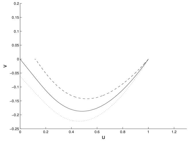
Fig. 1: Projection onto the $(u,v)$-plane of trajectories of (3) lying on different planes $H_{c}=c$. Here, $\beta=1$, and the three curves correspond to $c=0.5$ (dotted), $0.5707$ (solid) and $0.7$ (dashed).

Thus, we seek a heteroclinic solution of (3), which progresses between the fixed points $(1/\beta,0,0)$ and $(0,0,1)$, and is confined to the plane $\beta\,v+\beta\,c\,u+c\,y=c$; i.e., the fuel concentration obeys

$$y=1-\beta\,u-\frac{\beta}{c}\,v$$ (5)

at all values of $\xi$. Considering (3) under this restriction, we obtain

$$\left\{\begin{array}[]{lll}u^{\prime}&=&\displaystyle v\\ v^{\prime}&=&\displaystyle-\,c\,v-\left(1-\beta\,u-\frac{\beta}{c}\,v\right)\,e^{-1/u}\end{array}\right.\,.$$ (6)

This is effectively a projection of the flow on the particular invariant plane $H_{c}(u,v,y)$ $=c$ onto the $(u,v)$-plane. Any value of $c$ for which a heteroclinic connection exists between $(1/\beta,0)$ and $(0,0)$ is a permitted speed for the wavefront.

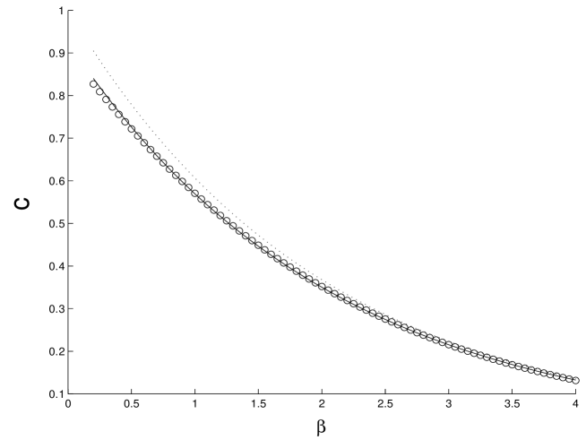
Fig. 2: Variation of the wavespeed $c$ with $\beta$: open circles (numerical results); unbroken curve (empirical curve (7)); dotted curve ($\exp(-0.5\beta)$, as obtained in [36, 7, 28]).

The unstable eigen-direction of the point $(1/\beta,0)$ is $(-c,-\beta e^{-\beta})$, and we determine $c$ numerically by shooting along this direction, and attempting to match up with a trajectory approaching the origin. In Figure 1 we show several numerically computed trajectories of this form, for different values of $c$, where we have chosen $\beta=1$. Note that this is not a standard $(u,v)$-phase space for (6), since each curve corresponds to a different value of the parameter $c$. Rather, it is a projection onto the $(u,v)$-plane of specialized trajectories from the invariant planes $H_{c}(u,v,y)=c$ of the three-dimensional system (3). The one trajectory which makes the required connection lies in the invariant plane corresponding to $c=0.5707$. The determination of this $c$ value was obtained by making incremental adjustments of $c$ until an appropriate connection is obtained.

We use this technique to numerically compute the wavespeeds for various values of the fuel parameter $\beta$, and illustrate this dependence in Figure 2. The wavespeed decays with $\beta$. For fuels with larger $\beta$ (poor fuels), the energy resulting from the reaction is insufficient to quickly activate combustion in nearby material, and combustion fronts propagate slowly. The data fits the exponential curve

$$c(\beta)=0.927\,e^{-0.486\beta}$$ (7)

with correlation $\rho>0.9999$. Equation (7) therefore provides an empirically determined formula of excellent accuracy, for the speed of a wavefront in perfectly solid adiabatic one-dimensional media. This result is close (and consistent with) a variety of sources: $\exp(-0.5\beta)$ is quoted in [36] for the small $\beta$ limit; this same value is given as an upper bound in [7], and also implied in eq. (10) in [28] using a large $\beta$ limit within a discontinuous front approximation. See Figure 2 for a comparison with our results.

The structure of the temperature front is illustrated in Figure 3 for $\beta=1$ (solid curve, left scale) and $\beta=3$ (dashed curve, right scale), demonstrating that larger $\beta$ fronts have a broader preheat layer preceding the front. Note that the preheat zone differs from the reaction zone [24]. The latter shrinks with increasing $\beta$ [13]. Specifically, the reaction zone as a fraction of the preheat zone is ${\mathcal{O}}(1/\beta)$ [24, 28]. The reaction zone is well localized near the region of greatest temperature change [24], and is not immediately identifiable in temperature profiles as in Figure 3. Indeed, the increase in size of the preheat layer with $\beta$ supports the ${\mathcal{O}}(1/\beta)$ expectation for the ratio between the reaction and the preheat zones.

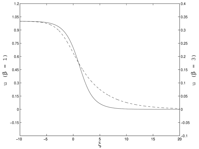
Fig. 3: Temperature front at $\beta=1$ (solid, left scale) and $\beta=3$ (dashed, right scale)

2.2 Wavespeed for $1\ll{\mbox{Le}}<\infty$

When the Lewis number is not infinite, but large, $\epsilon$ is small, and weak fuel diffusion needs to be permitted. This is a singular limit in (1) and (2), and as a consequence has been hardly examined in the literature. By defining $v=u^{\prime}$ as before, but now also $z=y^{\prime}$, the governing equations (2) can be represented as a four-dimensional system

$$\left\{\begin{array}[]{lll}u^{\prime}&=&\displaystyle v\\ v^{\prime}&=&\displaystyle-c\,v-y\,e^{-1/u}\\ y^{\prime}&=&\displaystyle z\\ z^{\prime}&=&\displaystyle\frac{1}{\epsilon}\left(-c\,z+\beta\,y\,e^{-1/u}\right)\end{array}\right.\,.$$ (8)

This is reducible to three-dimensions: the quantity

$$G_{c}^{\epsilon}(u,v,y,z)=\beta\,v+\beta\,c\,u+c\,y+\epsilon\,z$$

can be verified to be a conserved quantity of (8). Hence, flow is confined to the invariant three-dimensional surfaces $G_{c}^{\epsilon}=$ constant. Now, we seek a wavefront solution which goes from $(u,v,y,z)=(u_{B},0,0,0)$ to a value $(0,0,1,0)$, and we find that $G_{c}^{\epsilon}(u,v,y,z)=c$, and $u_{B}=1/\beta$ as before. The three-dimensional invariant surface on which both points lie is

$$z=\frac{1}{\epsilon}\left(c-\beta\,v-\beta\,c\,u-c\,y\right)\,.$$

The dynamics of (8) on this surface can be projected to the three variables $(u,v,y)$, such that

$$\left\{\begin{array}[]{lll}u^{\prime}&=&\displaystyle v\\ v^{\prime}&=&\displaystyle-c\,v-y\,e^{-1/u}\\ y^{\prime}&=&\displaystyle\frac{1}{\epsilon}\left(c-\beta\,v-\beta\,c\,u-c\,y\right)\end{array}\right.\,.$$ (9)

We seek the value of $c$ which permits a heteroclinic connection from $(u,v,y)=(1/\beta,0,0)$ to $(0,0,1)$. The former point (corresponding to $\xi=-\infty$) has only one positive eigenvalue, given by $(-c+\sqrt{c^{2}+4\epsilon\beta e^{-\beta}})/(2\epsilon)$. For small $\epsilon$, we “shoot” in the eigen-direction corresponding to this, with an initial guess of the wavespeed given by (7). Thereafter, as in the previous section, we adjust $c$ until we obtain a solution which approaches the point $(0,0,1)$ as $\xi\rightarrow\infty$. We do this numerically by considering the conditions $c\,y+\epsilon z=c$ and $v+c\,u=0$ which the front must obey at $\xi=+\infty$, and using a root-finding algorithm to adjust $c$. For a fixed value $\beta=1$, we illustrate how the wavespeed $c$ varies with $\epsilon$ in Figure 4, with the crosses. The dashed curve in Figure 4 is a analytical/numerical approximation we obtain for the wavespeed in terms of an explicit formula (18). The next two sections describe how we obtain this formula.

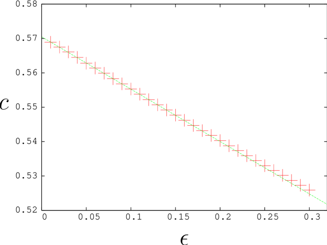
Fig. 4: Numerically computed wavespeed variation with $\epsilon$ for $\beta=1$ (the crosses). The dashed line is the theoretical approximation for $\beta=1$ obtained from the methods of Section 2.4.

We notice that $c$ decreases as we increase $\epsilon$, that is, when we decrease the Lewis number. Now, in dimensional form ${\mbox{Le}}=\kappa/(\rho\,c_{p}\,D)$, where $\rho,\kappa,c_{p}$ and $D$ are the respectively the density, thermal conductivity, specific heat capacity and molecular diffusivity of the fuel [37, 34, 8, 6, 30]. Increasing $\epsilon$ is equivalent to increasing the relative importance of $D$, $\rho$ and $c_{p}$ in relation to $\kappa$. Reducing $\kappa$ obviously decreases the ability of heat to move, and hence the combustion speed. Higher densities result in increased fuel mass in each location, which means more heat is needed in a given area to ignite all of the fuel before the wave moves on. Fuels with increased $c_{p}$ require more heat to increase the temperature by the a specified amount. Finally, increasing $D$ increases the transport of burnt fuel into the unburnt region and vice-versa, interfering with front propagation.

We computed the changes to the wavefront profile (akin to Figure 3) when $\epsilon$ is changed (not shown). We verified the obvious physical conclusion that the fuel concentration front becomes less steep when $\epsilon$ is increased from zero.

2.3 Slow manifold reduction

We now show that in the limit of small $\epsilon$, it is possible to further reduce the system (9) to a two-dimensional flow on a slow manifold. We begin with (9), and note that there are two “time”-scales in this singularly perturbed system, where we use “time” loosely to mean the independent variable $\xi$. We therefore adopt the standard dynamical systems trick of defining a new independent variable $\eta=\xi/\epsilon$ to elucidate motion in the fast “time” $\eta$. With a dot denoting the rate of change with respect to $\eta$, (9) becomes

$$\left\{\begin{array}[]{lll}\dot{u}&=&\epsilon\,v\\ \dot{v}&=&\epsilon\left(-c\,v-y\,e^{-1/u}\right)\\ \dot{y}&=&c-\beta\,v-\beta\,c\,u-c\,y\end{array}\right.\,.$$ (10)

In the $\epsilon=0$ limit, the system collapses to

$$\left\{\begin{array}[]{lll}\dot{u}&=&0\\ \dot{v}&=&0\\ \dot{y}&=&c-\beta\,v-\beta\,c\,u-c\,y\end{array}\right.\,,$$ (11)

in which it is clear that the plane ${\mathcal{S}}_{0}$ defined by $c-\beta\,v-\beta\,c\,u-c\,y=0$ consists entirely of fixed points. This is the same plane as defined through $H_{c}(u,v,y)=c$ for equation (3), on which the interesting behavior occurred for perfectly solid fuels. Each fixed point has a one-dimensional stable manifold (in the $y$-direction), and a two-dimensional center manifold, which is ${\mathcal{S}}_{0}$. Thus the plane ${\mathcal{S}}_{0}$ is invariant and normally hyperbolic with respect to (11); there is exponential contraction towards it as illustrated in Figure 5(a).

Fig. 5: The hyperbolic invariant manifold (a) ${\mathcal{S}}_{0}$ for (11), and (b) ${\mathcal{S}}_{\epsilon}$ for (10)

Upon switching on $\epsilon$ and considering the dynamics (10), ${\mathcal{S}}_{0}$ perturbs to an invariant curved entity ${\mathcal{S}}_{\epsilon}$, which is order $\epsilon$ away from ${\mathcal{S}}_{0}$. This is because of the structural stability of normally hyperbolic sets [18], which also implies that normal hyperbolicity is preserved for small $\epsilon$. Therefore, there is exponential decay of trajectories towards ${\mathcal{S}}_{\epsilon}$ on “time”-scales of order $\eta$, as shown in Figure 5(b). Motion on ${\mathcal{S}}_{\epsilon}$ occurs at a slower rate (on “time”-scales of order $\xi$), and hence it is termed a ‘slow manifold’. The heteroclinic connection we seek lies on ${\mathcal{S}}_{\epsilon}$, from $(u,v,y)=(1/\beta,0,0)$ to $(0,0,1)$. Since ${\mathcal{S}}_{\epsilon}$ is invariant, two-dimensional and not parallel to the $y$-axis, it therefore makes sense to project the motion to the $(u,v)$-plane in order to describe behavior. To elucidate this motion, we need to once again return to the original “time”-scale $\xi$ – the slow time associated with motion on the slow manifold.

Return to the relationship $G_{c}^{\epsilon}\left(u(\xi),v(\xi),y(\xi),z(\xi)\right)=c$, which upon differentiation yields

$$\beta\,v^{\prime}+\beta\,c\,u^{\prime}+c\,y^{\prime}+\epsilon\,z^{\prime}=0\,,$$

and since $u^{\prime}=v$ and $y^{\prime}=z$,

$$z=-\frac{\beta}{c}\,v^{\prime}-\beta\,v-\frac{\epsilon}{c}z^{\prime}\,.$$

Substituting back into $G_{c}^{\epsilon}(u,v,y,z)=c$, we obtain

$$\beta\,v+\beta\,c\,u+c\,y+\epsilon\left(-\frac{\beta}{c}\,v^{\prime}-\beta\,v+{\mathcal{O}}(\epsilon)\right)=c\,,$$

and thus

$$y=1-\frac{\beta}{c}\,v-\beta\,u+\epsilon\,\frac{\beta}{c^{2}}\,v^{\prime}+\epsilon\,\frac{\beta}{c}\,v+{\mathcal{O}}(\epsilon^{2})\,.$$

Substitution into the $v^{\prime}$ equation in (8) or (9) gives

$$v^{\prime}\left(1+\epsilon\,\frac{\beta}{c^{2}}e^{-1/u}\right)=-c\,v-\left(1-\frac{\beta}{c}\,v-\beta\,u+\epsilon\,\frac{\beta}{c}\,v+{\mathcal{O}}(\epsilon^{2})\right)e^{-1/u}\,.$$

Therefore

$$v^{\prime} = \left(1-\epsilon\,\frac{\beta}{c^{2}}e^{-1/u}\right)\left[-c\,v-\left(1-\frac{\beta}{c}\,v-\beta\,u+\epsilon\,\frac{\beta}{c}\,v\right)e^{-1/u}\right]+{\mathcal{O}}(\epsilon^{2})$$

$$= -c\,v-\left(1-\frac{\beta}{c}\,v-\beta\,u\right)e^{-1/u}+\epsilon\,\frac{\beta}{c^{2}}\left(1-\frac{\beta}{c}\,v-\beta\,u\right)e^{-2/u}+{\mathcal{O}}(\epsilon^{2})\,.$$

Retaining only ${\mathcal{O}}(\epsilon)$ terms, we obtain the $(u,v)$-projected approximate equations on the slow manifold

$$\left\{\begin{array}[]{lll}u^{\prime}&=&\displaystyle v\\ v^{\prime}&=&\displaystyle-c\,v-\left(1-\frac{\beta}{c}v-\beta\,u\right)e^{-1/u}+\epsilon\,\frac{\beta}{c^{2}}\left(1-\frac{\beta}{c}\,v-\beta\,u\right)e^{-2/u}\end{array}\right.\,.$$ (12)

We will now show how to use these approximate dynamics to predict the correction to the wavespeed resulting from the inclusion of the finiteness of the Lewis number.

2.4 Perturbative formula for wavespeed

Here, we derive and numerically study a formula for the wavespeed correction in going from ${\mbox{Le}}=\infty$ to finite Lewis number. Let

$$c\left(\beta,\epsilon\right)=c_{0}\left(\beta\right)+\epsilon\,c_{1}\left(\beta\right)+{\mathcal{O}}\left(\epsilon^{2}\right)\,,$$ (13)

where $c_{0}$ is the wavespeed associated with the infinite Lewis number ($\epsilon=0$) combustion wavefront. In the spirit of perturbation analysis, we obtain a formula for the correction $c_{1}(\beta)$ purely in terms of the unperturbed ($\epsilon=0$) wave, using a nontraditional application of “Melnikov’s method” [29] from dynamical systems theory.

Melnikov’s method is applied most commonly to area-preserving two-dimensional systems under time-periodic perturbations [21, 4, 38]. (Here, once again, $\xi$ represents “time”.) Our system (12) is not area-preserving, and has a perturbation which is independent of the temporal variable. Under these conditions, we describe the method applied to the system

$${\mathbf{z}}^{\prime}={\mathbf{f}}\left({\mathbf{z}}\right)+\epsilon\,{\mathbf{g}}\left({\mathbf{z}}\right)\,.$$ (14)

When $\epsilon=0$, suppose this system possesses a heteroclinic connection between the two saddle fixed points ${\mathbf{a}}$ and ${\mathbf{b}}$ as shown in Figure 6(a). A heteroclinic connection of this sort occurs when a branch of the one-dimensional unstable manifold of ${\mathbf{a}}$ coincides with a branch of the stable manifold of ${\mathbf{b}}$. This heteroclinic trajectory can be represented as a solution ${\mathbf{z}}=\hat{\mathbf{z}}(\xi)$ to (14) with $\epsilon=0$.

Fig. 6: Manifold structure for the Melnikov approach: (a) $\epsilon=0$, (b) $\epsilon\neq 0$

Now, for small $\epsilon>0$ in (14), the fixed points ${\mathbf{a}}$ and ${\mathbf{b}}$ perturb by ${\mathcal{O}}(\epsilon)$, and retain their stable and unstable manifolds [18]. However, these need no longer coincide. Figure 6(b) shows how they can split apart, with the dashed curve showing the original manifold. Let $d(\xi,\epsilon)$ be a distance measure between these manifolds, measured along a perpendicular to the unperturbed heteroclinic drawn at $\hat{\mathbf{z}}(-\xi)$. The variable $\xi$ can thus be used to identify the position along the heteroclinic curve (cf. “heteroclinic coordinates” of Section 4.5 in [38]). Since $d(\xi,0)=0$ for all $\xi$, this distance is Taylor expandable in $\epsilon$ in the form

$$d(\xi,\epsilon)=\epsilon\,\frac{M(\xi)}{\left|{\mathbf{f}}\left(\hat{\mathbf{z}}(-\xi)\right)\right|}+{\mathcal{O}}(\epsilon^{2})\,,$$

where the scaling factor $\left|f\left(\hat{\mathbf{z}}(-\xi)\right)\right|$ in the denominator represents the unperturbed trajectory’s speed at the location $\xi$. The quantity $M(\xi)$ is the “Melnikov function”, for which an expression is

$$M\left(\xi\right)=\int_{-\infty}^{\infty}\exp\left[-\int_{-\xi}^{\mu}{\mathbf{\nabla}}\cdot{\mathbf{f}}(\hat{\mathbf{z}}(s))\,ds\right]{\mathbf{f}}(\hat{\mathbf{z}}(\mu))\wedge{\mathbf{g}}(\hat{\mathbf{z}}(\mu))\,d\mu\,,$$ (15)

where the wedge product between two vectors is defined by $(a_{1},a_{2})^{T}\wedge(b_{1},b_{2})^{T}=a_{1}b_{2}-a_{2}b_{1}$. Obtaining the version (15) requires two adjustments to the standard Melnikov approaches [21, 4, 38]: incorporating the non area-preserving nature of the unperturbed flow of (14), and representing the distance in terms of heteroclinic coordinates. Details are provided in Appendix A. We need to ensure the persistence of a heteroclinic trajectory in (12) for $\epsilon>0$, and thus require $d(\xi,\epsilon)=0$ for all $\xi$. For this to happen for all small $\epsilon$, we therefore need to set $M(\xi)\equiv 0$.

To apply this technique to our system, we begin by writing (12) in the form (14). Using the expansion (13), and utilizing binomial expansions for $1/(c_{0}+\epsilon c_{1})$, we get

$$\left\{\begin{array}[]{lll}\displaystyle u^{\prime}&=&\displaystyle v\\ \displaystyle v^{\prime}&=&\displaystyle-c_{0}\,v-e^{-1/u}\Upsilon_{uv}+\epsilon\left(-c_{1}v-\frac{\beta c_{1}e^{-1/u}}{c_{0}^{2}}v+\frac{\beta e^{-2/u}}{c_{0}^{2}}\Upsilon_{uv}\right)\end{array}\right.\,,$$ (16)

where higher-order terms in $\epsilon$ have been discarded, and

$$\Upsilon_{uv}=1-\beta\,u-\frac{\beta}{c_{0}}\,v\,.$$

By appropriately identifying ${\mathbf{f}}$ and ${\mathbf{g}}$ from (16) through comparison with (14), we see that

$$\left({\mathbf{f}}\wedge{\mathbf{g}}\right)(u,v)=v\left(-c_{1}v-\frac{\beta c_{1}e^{-1/u}v}{c_{0}^{2}}+\frac{\beta e^{-2/u}}{c_{0}^{2}}\Upsilon_{uv}\right)$$

and ${\mathbf{\nabla}}\cdot{\mathbf{f}}=-c_{0}+\beta e^{-1/u}/c_{0}$. Substituting into the Melnikov formula (15), and setting it equal to zero, we obtain

$$\int_{-\infty}^{\infty}\exp\left[\int_{-\xi}^{\mu}\left(c_{0}-\frac{\beta}{c_{0}}e^{-1/u(s)}\right)ds\right]v\left(-c_{1}v-\frac{\beta vc_{1}e^{-1/u}}{c_{0}^{2}}+\frac{\beta e^{-2/u}}{c_{0}^{2}}\Upsilon_{uv}\right)\,d\mu=0\,,$$

where each of $u(\mu)$ and $v(\mu)$ is evaluated along the $\epsilon=0$ combustion wave. Notice, however, that for this infinite Lewis number combustion wave, (5) tells us that the fuel concentration $y(\mu)=\Upsilon_{uv}(\mu)$ for all $\mu$. Therefore

$$c_{1}(\beta)=\beta\,\frac{\displaystyle\int_{-\infty}^{\infty}\exp\left[\int_{-\xi}^{\mu}\left(c_{0}-\frac{\beta}{c_{0}}e^{-1/u(s)}\right)\,ds\right]v\,y\,e^{-2/u}\,d\mu}{\displaystyle\int_{-\infty}^{\infty}\exp\left[\int_{-\xi}^{\mu}\left(c_{0}-\frac{\beta}{c_{0}}e^{-1/u(s)}\right)\,ds\right]v^{2}(c_{0}^{2}+\beta\,e^{-1/u})\,d\mu}\,,$$ (17)

where $u(\mu)$, $v(\mu)$ and $y(\mu)$ in the integrands are obtained from the $\epsilon=0$ combustion wave discussed in Section 2.1. The apparent dependence of $c_{1}$ on the wave coordinate $\xi$ is spurious: if $I$ is an anti-derivative of the inner integrals in (17), a multiplicative term $\exp\left[-I(-\xi)\right]$ emerges in both the numerator and denominator, which therefore cancels. Hence, any convenient value for $\xi$ can be chosen in (17), for example $0$.

Equation (17) is a powerful expression in which the wavespeed correction is expressed purely in terms of the (unperturbed) infinite Lewis number wavefront and system parameters. This correction was obtained through an application of the slow manifold and Melnikov’s method (suitably modified). While developed within the current specific context, we note that this technique can in fact be used in a variety of instances which are modeled through coupled reaction-diffusion equations in which the diffusivities are very different.

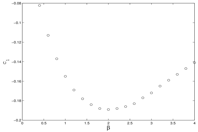
Fig. 7: The perturbing wavespeed as a function of $\beta$

We note that $v<0$ for the infinite Lewis number wavefront, as is clear from the phase-portrait Figure 1. Alternatively, $u$ is smaller at the front of the wave, where fuel is yet to be burnt, and is therefore a decreasing function of $\mu$, leading to $v=u^{\prime}<0$. Based on this, (17) immediately displays that $c_{1}<0$, proving the property that the wavespeed decreases when fuel diffusivity is included. This is in agreement with the numerical observations in Section 2.2.

Equation (17) provides an explicit perturbative formula on how the wavespeed varies through the inclusion of the finiteness of the Lewis number, expressed entirely in terms of the infinite Lewis number combustion wave. This result is used to compute the solid line in Figure 4, which is the theoretical wavespeed $0.5707-0.1552\epsilon$ obtained by using (17) and (13) when $\beta=1$. When $\epsilon$ is small, it forms an excellent approximation to the numerically obtained wavespeed, as described in Section 2.2. Indeed, Figure 4 show that the theoretical line is tangential to the curve formed by the closed circles.

The perturbation wavespeed $c_{1}$ as a function of $\beta$ appears in Figure 7. There is a value of $\beta$ (around $2$) at which the absolute influence of the finiteness of the Lewis number is greatest. Nevertheless, since $c_{0}$ is itself a function of $\beta$, it makes sense to investigate the relative influence $c_{1}/c_{0}$ of the perturbative term. Such is presented in the numerically computed Figure 8. The graph is virtually linear and has zero intercept. In other words, the complicated quotient in (17) is in fact proportional to the unperturbed wavespeed $c_{0}(\beta)$, with the proportionality factor independent of $\beta$. We therefore arrive at the approximation

$$c(\beta,\epsilon)=c_{0}(\beta)\left[1-0.267\,\epsilon\,\beta\right]=c_{0}(\beta)\left[1-0.267\,\frac{\beta}{{\mbox{Le}}}\right]\,,$$ (18)

for large Lewis numbers, with excellent validity across all $\beta$, and with $c_{0}(\beta)$ also known through (7).

Equation (18) shows that the wavespeed, as a fraction of the infinite Lewis number wavespeed, acquires a correction linear in the ratio $\beta/{\mbox{Le}}$. We are not aware of any such result being previously reported in the literature of combustion waves. Moreover, the simplicity of this expression is remarkable. For the specific instance $\beta=1$, we apply this formula in order to arrive at the dashed line in Figure 4. Our perturbative theory has clearly given us a very accurate and simple approximation, and elucidates the straightforward dependence of the wavespeed on the parameters $\beta$ and Le.

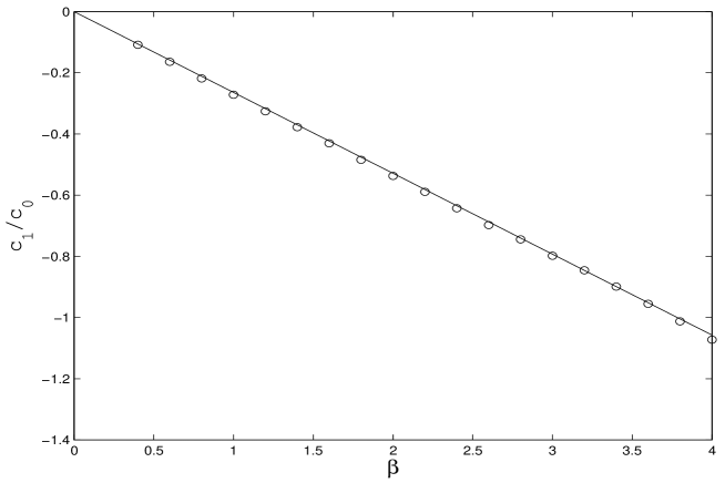
Fig. 8: Relative size of perturbative wavespeed as a function of $\beta$

3 Stability analysis

In this section, we test the stability of the combustion wavefront $(u,y)=\left(u_{0}(\xi),y_{0}(\xi)\right)$ we have found as a solution to (1) at large Lewis numbers. Consider a perturbation of the form

$$u=u_{0}(\xi)+U(\xi)\,e^{\lambda\,t},\;\;y=y_{0}(\xi)+Y(\xi)\,e^{\lambda\,t}.$$ (19)

At first order, $U$ and $Y$ satisfy an eigenvalue problem

$$\left(\begin{array}[]{l}U\\ V\\ Y\\ Z\end{array}\right)^{\prime}=\left(\begin{array}[]{ccccccc}0&&1&&0&&0\\ \lambda-\frac{y_{0}}{u_{0}^{2}}\,e^{-1/u_{0}}&&-c&&-e^{-1/u_{0}}&&0\\ 0&&0&&0&&1\\ \frac{\beta\,y_{0}}{\epsilon\,u_{0}^{2}}\,e^{-1/u_{0}}&&0&&\frac{\lambda}{\epsilon}+\frac{\beta}{\epsilon}\,e^{-1/u_{0}}&&-\frac{c}{\epsilon}\end{array}\right)\left(\begin{array}[]{l}U\\ V\\ Y\\ Z\end{array}\right).$$ (20)

Linear instability occurs if there are values of $\lambda$ in the right half plane for which (20) possesses a solution uniformly bounded for all $\xi$. It turns out that such values of $\lambda$ can be investigated by analyzing the Evans function [17], which is a complex analytic function $E(\lambda)$ whose zeros correspond to exactly these $\lambda$ values. If for example it can be shown that $E(\lambda)$ has no zeros in the right half plane, the indications from the point spectrum of (20) is that the wavefront is stable. If there exist zeros of $E(\lambda)$ in the right half plane, the wavefront is unstable. A description of the Evans function as used in our study is given in Appendix B. This was proposed in [2, 16, 23, 40] and has been used by [20] for a detailed numerical analysis of (1). (It must be also mentioned that in the linear stability analysis, it is necessary to consider the essential spectrum associated with (20); it turns out that this has no intersection with the right half plane and therefore need not worry us further.)

We begin with a traveling wave solution $u_{0}(\xi)$ and $y_{0}(\xi)$ obtained using standard shooting methods in Section 2, and then compute the Evans function using the procedure outlined in Appendix B. We note that the system is very sensitive due to its stiffness. We found a solution to be accurate enough if we obtain $E(\lambda=0)\sim{\cal{O}}(10^{-12})$. We are guided in our calculations by the detailed stability analysis of Gubernov et al [20]. They show, for example, the lack of any eigenvalues of positive real part for small $\beta$, but show that for $\beta$ large enough, two eigenvalues pop into the right half plane exhibiting a Hopf bifurcation. Physically, this corresponds to a pulsating instability in the wavefront, a well known phenomenon also occurring for ${\mbox{Le}}=\infty$ even in slightly different models [37, 14, 28, 5]. Gubernov et al extend these infinite Lewis number analyses by producing in Figure 5 in [20] the stability boundary in $\beta$-$\epsilon$ space (their $\tau$ is our $\epsilon$). We verify here that our numerically computed wavefronts display the characteristics outlined by them.

In Figure 9 we show the Evans function $E(\lambda)$ as it varies with increasing $\lambda\in{\mathbb{R}}$ for ${\mbox{Le}}=17$ and $\beta=1$ (this corresponds to a stable regime in Figure 5 of [20]). We find that Evans function does not have any positive real roots. To test for complex roots we vary $\lambda\in i{\mathbb{R}}$; using Cauchy’s theorem we can calculate the winding number to detect possible oscillatory instabilities. In the left panel of Figure 10 we show the complex Evans function. Since the system (1) is translationally invariant, the Evans function has at least a simple zero at $\lambda=0$. We checked with a little off-set of the order ${\cal{O}}(10^{-5})$ whether the (real) value of the Evans function at $\lambda=0$ is shifting towards larger values or smaller values. The off-set allows us to integrate parallel to the imaginary axis of $\lambda$ and therefore excluding the zero of the Evans function stemming from the root at $\lambda=0$. This enables us to attribute roots of the Evans function to either the translational mode or to a real instability. For the case depicted in Figure 10 we find that the Evans function moves to the right. This means that the Evans function can be cast in the topologically equivalent form depicted in the right panel of Figure 10 and it has clearly a winding number zero. We therefore find that at these parameter values there are no unstable eigenvalues. (Note that for this argument to work we need our definition of the Evans function to be analytic which excludes standard methods such as Gram-Schmidt orthogonalizations.)

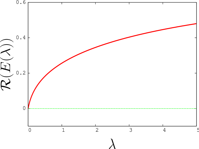
Fig. 9: The real part of the Evans function $E(\lambda)$ for ${\mbox{Le}}=17$ and $\beta=1$ as a function of $\lambda$.

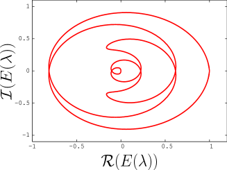
Fig. 10: Left: The real versus the imaginary part of the Evans function $E(\lambda)$ for ${\mbox{Le}}=17$ and $\beta=1$. The spectral parameter $\lambda$ varies along the imaginary axis. Right: A sketch of a topologically equivalent Evans function. The winding number is clearly zero indicating stability.

We next choose ${\mbox{Le}}=100$ and $\beta=9$, parameters at which (according to Figure 5 in [20]) an oscillatory instability is to be expected. In Figure 11 we show the Evans function in this situation, with a zoom in displayed in Figure 12. To determine the winding number we need to check whether the small circle of the Evans function in Figure 12 includes the zero or not. We can do so by allowing again for a small off-set of $\lambda$. We find that the circle includes zero. Unfolding the behavior of the Evans function then allows to sketch a topologically equivalent Evans function as in the right panel of Figure 12. We verified that the instability is indeed oscillatory by examining the Evans function for $\lambda\in{\mathbb{R}}^{+}$, which reveals no zeros. Hence our wavefront displays the predicted characteristics of [20]. Stability properties are not affected unduly by the finiteness of the Lewis number, despite the singularity of this limit.

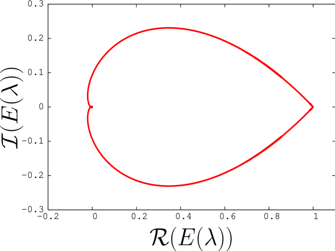
Fig. 11: The real versus the imaginary part of the Evans function $E(\lambda)$ for ${\mbox{Le}}=100$ and $\beta=9$. The spectral parameter $\lambda$ varies along the imaginary axis.

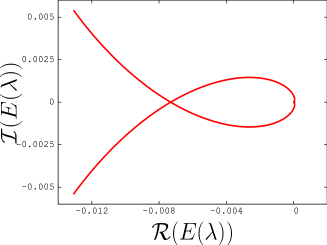
Fig. 12: Left: Closeup of the Evans function depicted in Fig. 11 into the region $E(\lambda)=0$. Right: A sketch of a topologically equivalent Evans function. The winding number is clearly two indicating an oscillatory instability.

4 Concluding remarks

In this article, we have studied combustion wavefront in a one-dimensional medium. Our concentration was on very high Lewis numbers relevant to high-density supercritical combustion. We determine the wavespeed as a function of the exothermicity parameter $\beta$ and the Lewis number Le, by seeking the wavespeed value which establishes a connection between the fixed points corresponding to the fully burnt and the unburnt states. The infinite Lewis number instance reveals an exponential dependence of the wavespeed on $\beta$, for which we determine an empirical formula. We then use several suitably modified dynamical systems techniques (slow manifold reduction, and Melnikov’s method) to compute an explicit formula (17) for the correction to the wavespeed when including the effect of large, but not infinite, Lewis number. We hence obtain a simple formula (18) which shows that the relative change in the wavespeed is proportional to $\beta/{\mbox{Le}}$ for large Lewis numbers. Our theory is shown to have excellent consistency with the numerically computed wavespeed for large Le, as we show in Figure 4.

The stability of the high Lewis number wavefronts is then tested numerically based on the Evans function technique. Our results are in agreement with the stability boundaries presented by Gubernov et al in Figure 5 in [20].

We remark that the modified Melnikov’s method that we have used can in fact be used in more general situations which are described by two coupled reaction-diffusion equations with strongly differing diffusivities. Based on a known wavefront or wave-pulse solution for when the smaller of the diffusivities is zero, our technique can in some instances be used to determine the wavespeed correction resulting from the inclusion of the (previously neglected) diffusivity. Alternatively, it can be adapted to situations in which the wavespeed changes due to some other small parameter. Our analysis of high Lewis number wavefronts therefore provides a new perturbative methodology for analyzing certain classes of reaction-diffusion equations, pattern formation problems and combustion waves.

Acknowledgements
The authors wish to thank Harvinder Sidhu, Konstantina Trivisa, Marshall Slemrod, and Joceline Lega for discussions and pointers. Detailed comments and suggestions from two anonymous referees, whose efforts revealed a substantial error in a previous version of this manuscript, are also gratefully acknowledged. Part of this work was done while S.L. was visiting the School of Mathematics and Statistics at the University of Sydney and while S.B. was visiting the Department of Mathematics at the College of Charleston. This material is based upon work supported by the National Science Foundation under Grant No. DMS-0509622 to S.L. G.A.G. gratefully acknowledges support by the Australian Research Council, DP0452147.

Appendix A Melnikov function derivation

We briefly outline the modifications needed to the standard Melnikov approaches [21, 4, 38] relevant to Section 2.4. Our system is $\dot{\mathbf{z}}=f\left({\mathbf{z}}\right)+\epsilon\,g\left({\mathbf{z}}\right)$, as given in (14). Consider a particular parametrization of the heteroclinic $\hat{\mathbf{z}}(\xi)$. Imagine the perturbed system as embedded in three-dimensional $\left({\mathbf{z}},s\right)$ space. In a “time”-slice $s=s_{0}$, let ${\mathcal{T}}$ be the normal vector to the heteroclinic drawn at the point $\hat{\mathbf{z}}(0)={\mathbf{z}}_{0}$. The usual approach is to compute the distance between the perturbed manifolds measured along ${\mathcal{T}}$, and this is expandable as

$$d(s_{0},\epsilon)=\epsilon\,\frac{M(s_{0})}{\left|{\mathbf{f}}\left({\mathbf{z}}_{0}\right)\right|}+{\mathcal{O}}(\epsilon^{2})\,.$$ (21)

Let ${\mathbf{z}}^{u}(s)$ be the trajectory of the perturbed flow which intersects ${\mathcal{T}}$ and which backwards asymptotes to the perturbed fixed point ${\mathbf{a}}(\epsilon)$. In other words, ${\mathbf{z}}^{u}(s)$ is a trajectory lying on ${\mathbf{a}}(\epsilon)$’s unstable manifold. The standard approach [21, 4] is to represent

$${\mathbf{z}}^{\sigma}(s)=\hat{\mathbf{z}}(s-s_{0})+\epsilon\,{\mathbf{z}}_{1}^{\sigma}(s)+{\mathcal{O}}(\epsilon^{2})$$

where $\sigma=u$ (for “unstable”), valid for $-\infty<s\leq s_{0}$ . A similar expansion on $s_{0}\leq s<\infty$ with $\sigma=s$ (for “stable”), works for the trajectory ${\mathbf{z}}^{s}(s)$, which intersects ${\mathcal{T}}$ on the time-slice $s_{0}$ and which lies on the stable manifold of the perturbed fixed point ${\mathbf{b}}(\epsilon)$. Then, the standard Melnikov development (see [21, 4]) allows the representation

$$d(s_{0},\epsilon)=\epsilon\,\frac{\Delta^{u}(s_{0})-\Delta^{s}(s_{0})}{\left|{\mathbf{f}}\left({\mathbf{z}}_{0}\right)\right|}+{\mathcal{O}}(\epsilon^{2})\,,$$ (22)

where

$$\Delta^{\sigma}(s)={\mathbf{f}}\left(\hat{\mathbf{z}}(s-s_{0})\right)\wedge{\mathbf{z}}_{1}^{\sigma}(s)$$

for $\sigma=u$ and $\sigma=s$. Now, [21, 4] derive that

$$\dot{\Delta}^{\sigma}={\mathbf{\nabla}}\cdot{\mathbf{f}}\left(\hat{\mathbf{z}}(s-s_{0})\right)\,\Delta^{\sigma}+{\mathbf{f}}\left(\hat{\mathbf{z}}(s-s_{0})\right)\wedge{\mathbf{g}}\left(\hat{\mathbf{z}}(s-s_{0}),s\right)+{\mathcal{O}}(\epsilon)$$ (23)

but since the unperturbed dynamical system is volume-preserving, have the luxury of ignoring the first term on the right hand side. We cannot do so here, but we can neglect the second argument in ${\mathbf{g}}$ since our case is autonomous. To deal with the first term, we multiply (23) by the integrating factor

$$\mu(s)=\exp\left[-\int_{0}^{s}{\mathbf{\nabla}}\cdot{\mathbf{f}}\left(\hat{\mathbf{z}}(r-s_{0})\right)\,dr\right]$$

before proceeding. Having done so, we integrate from $-\infty$ to $s_{0}$ by choosing $\sigma=u$, then integrate from $s_{0}$ to $\infty$ by choosing $\sigma=s$, and then add the two equations to get

$$\Delta^{u}(s_{0})-\Delta^{s}(s_{0})=\int_{-\infty}^{\infty}\frac{\mu(s)}{\mu(s_{0})}{\mathbf{f}}\wedge{\mathbf{g}}\left(\hat{\mathbf{z}}(s-s_{0})\right)\,ds\,.$$

(This is an adaptation of the standard process [21, 4].) In conjunction with (21) and (22), and also employing the shift $s-s_{0}\rightarrow s$ in the integrand, we obtain the Melnikov function

$$M(s_{0})=\int_{-\infty}^{\infty}\exp\left[-\int_{0}^{s}{\mathbf{\nabla}}\cdot{\mathbf{f}}\left(\hat{\mathbf{z}}(r)\right)\,dr\right]{\mathbf{f}}\wedge{\mathbf{g}}\left(\hat{\mathbf{z}}(s)\right)ds\,$$

which no longer depends on $s_{0}$. Having dealt with the non volume-preserving instance, the next step is to change our attitude: rather than measuring the distance in a time-slice $s$ but at a specific point ${\mathbf{z}}_{0}$, we ignore time-slices (since our perturbed system is itself autonomous), and allow the point to vary along the heteroclinic. To do so, choose a different parametrization $\hat{\mathbf{w}}(s)=\hat{\mathbf{z}}(s-\xi)$ of the heteroclinic. Thus, the point ${\mathbf{w}}_{0}=\hat{\mathbf{w}}(0)=\hat{\mathbf{z}}(-\xi)$ can be varied along the heteroclinic by choosing different values of $\xi$. Therefore, $\xi$ will represent different points along the heteroclinic at which the distance measurement is to be made (cf. “heteroclinic coordinates” of [38]). Using the ${\mathbf{w}}$ trajectory, our earlier results can be expressed as

$$d(s_{0},\xi)=\epsilon\,\frac{M(s_{0},\xi)}{\left|{\mathbf{f}}\left({\mathbf{w}}_{0}\right)\right|}+{\mathcal{O}}(\epsilon^{2})=\epsilon\,\frac{M(\xi)}{\left|{\mathbf{f}}\left({\mathbf{z}}(-\xi)\right)\right|}+{\mathcal{O}}(\epsilon^{2}),\,,$$ (24)

where

$$M(\xi) = \int_{-\infty}^{\infty}\exp\left[-\int_{0}^{s}{\mathbf{\nabla}}\cdot{\mathbf{f}}\left(\hat{\mathbf{w}}(r)\right)dr\right]{\mathbf{f}}\wedge{\mathbf{g}}\left(\hat{\mathbf{w}}(s)\right)ds$$

$$= \int_{-\infty}^{\infty}\exp\left[-\int_{0}^{s}{\mathbf{\nabla}}\cdot{\mathbf{f}}\left(\hat{\mathbf{z}}(r-\xi)\right)dr\right]{\mathbf{f}}\wedge{\mathbf{g}}\left(\hat{\mathbf{z}}(s-\xi)\right)ds$$

$$= \int_{-\infty}^{\infty}\exp\left[-\int_{0}^{s+\xi}{\mathbf{\nabla}}\cdot{\mathbf{f}}\left(\hat{\mathbf{z}}(r-\xi)\right)dr\right]{\mathbf{f}}\wedge{\mathbf{g}}\left(\hat{\mathbf{z}}(s)\right)ds$$

$$= \int_{-\infty}^{\infty}\exp\left[-\int_{-\xi}^{s}{\mathbf{\nabla}}\cdot{\mathbf{f}}\left(\hat{\mathbf{z}}(r)\right)dr\right]{\mathbf{f}}\wedge{\mathbf{g}}\left(\hat{\mathbf{z}}(s)\right)ds\,.$$

This, in conjunction with (24), is the expression used in Section 2.4.

Appendix B Evans function definition

Here, we describe the Evans function approach for analyzing linear stability. In general, the linear stability of a localized traveling wave solution to a system of PDEs is obtained by studying the eigenvalue problem

$${\cal{L}}\,w=\lambda\,w\,,$$ (25)

where the matrix differential operator ${\cal{L}}$ arises from the linearization of the PDEs. The traveling solution is said to be linearly stable if the spectrum of $\cal{L}$ lies in the closed left half-plane.

The system (25) can be turned into a linear dynamical system of the form

$$U_{\xi}={\bf A}(\xi,\lambda)\,U$$ (26)

where ${\bf A}(\xi,\lambda)$ is an $n\times n$ square matrix depending on $\xi=x-c\,t$ and the spectral parameter $\lambda$ (in our case, $n=4$). It can be shown that the asymptotic behavior of the solutions to (26) is determined by the matrices

$${\bf A}_{\pm\infty}(\lambda)=\lim_{\xi\rightarrow\pm\infty}{\bf A}(\xi,\lambda)$$

in the following sense (see [11] for details). If $\mu^{+}$ (resp. $\mu^{-}$) is an eigenvalue of ${\bf A}_{+\infty}$ (resp. ${\bf A}_{-\infty}$) with eigenvector $v^{+}$ (resp. $v^{-}$), then there exists a solution $w^{+}$ (resp. $w^{-}$) to (26) with the property that

$$\lim_{\xi\rightarrow\infty}w^{+}e^{-\mu^{+}\,\xi}=v^{+}\;\;\;\left({\mbox{resp.}}\;\;\lim_{\xi\rightarrow-\infty}w^{-}e^{-\mu^{-}\,\xi}=v^{-}\right)\,.$$ (27)

Note that the superscript “$+$” refers to exponentially decaying behavior at $\xi=+\infty$, while “$-$” refers to $\xi=-\infty$.

To study the linear stability, one should consider both the essential and point spectrum of $\cal{L}$. The essential spectrum of ${\cal{L}}$ consists of the values of $\lambda$ for which ${\bf A}_{\infty}$ or ${\bf A}_{-\infty}$ has purely imaginary eigenvalues [22]. The point spectrum can be studied by means of the Evans function, first introduced by Evans [16] and later generalized [2]. Roughly speaking, the zeros of this complex-valued function are arranged to coincide with the point spectrum of $\cal{L}$.

Let $\Omega$ denote a domain of the complex $\lambda$ plane with no intersection with the essential spectrum and let $n_{s}$ and $n_{u}$ denote, respectively, the number of eigenvalues of ${\bf A}_{\infty}$ with negative real part and the number of eigenvalues of ${\bf A}_{-\infty}$ with positive real part in $\Omega$. We assume that $n_{s}+n_{u}=n$. Let $w_{i}^{+}(\lambda,\xi)$, $i=1,2,...,n_{s}$ (resp. $w_{i}^{-}(\lambda,\xi)$, $i=1,2,...,n_{u}$) be linearly independent solutions to (26) converging to zero as $\xi\rightarrow\infty$ (resp. $\xi\rightarrow-\infty$) which are analytic of $\lambda$ in $\Omega$. Clearly, a particular value of $\lambda$ belongs to the point spectrum of $\cal{L}$ if (26) admits a solution that is converging to zero for both $\xi\rightarrow\pm\infty$, that is if the space of solutions generated by the $w_{i}^{+}$ intersects with the one generated by the $w_{i}^{-}$. To detect such values of $\lambda$ in $\Omega$, one can use the definition of the Evans function given in [33]

$$E(\lambda)=\det{\left(w_{1}^{+},w_{2}^{+},...w_{n_{s}}^{+},w_{1}^{-},w_{2}^{-},...w_{n_{u}}^{-}\right)},$$

in which the $w_{i}^{\pm}$ are evaluated at $\xi=0$. This function is analytic in $\Omega$, is real for real values of $\lambda$ and the locations of the zeros of $E(\lambda)$ correspond to eigenvalues of $\cal{L}$.

The first numerical computation of the Evans function was by Evans himself in [17], and followed by [35, 32]. However, in all three papers $n_{s}=1$, in which case a standard shooting argument can be used. In standard shooting algorithms one follows the stable and/or unstable manifolds at $\xi=\pm\infty$. The Evans function is then given as the intersection of these manifolds. As shown in Section 3, our system has $n=4$ and $n_{s}=n_{u}=2$. This causes the following practical problem: although the $n_{s}$ (or $n_{u}$ respectively) eigenvectors are linear independent solutions of the eigenvalue problem (26) at $\xi=\pm\infty$, the numerical integration scheme will lead to an inevitable alignment with the eigen-direction corresponding to the largest eigenvalue. This collapse of the eigen-directions is usually overcome by using Gram-Schmidt orthogonalization. However, this is not desirable for calculating the Evans function as it is a nonanalytic procedure which then subsequently prohibits the use of Cauchy’s theorem (argument principle) to locate complex zeros of the Evans function. The Evans function is therefore best calculated using exterior algebra [31, 9, 12, 1, 3, 11, 15, 34].

We briefly review the method here, with specific regard to the situation in which $n=4$ and $n_{s}=n_{u}=2$. For more details the reader is referred to [1, 3, 11, 15], and to the numerical computation in [20]. The main idea behind exterior algebra methods (or compound matrices methods) is that the linear system (26) induces a dynamical system on the wedge-space $\bigwedge^{2}({\mathbb{C}}^{4})$ for $n_{s}=n_{u}=2$. The wedge-space $\bigwedge^{2}({\mathbb{C}}^{4})$ is the space of all two forms on ${\mathbb{C}}^{n}$. This is a space of dimension ${4\choose 2}=6$. The induced dynamics on the wedge-space $\bigwedge^{2}({\mathbb{C}}^{4})$ can be written as

$${\bf U}_{\xi}={\bf A}^{(2)}(\xi){\bf U},\quad{\bf U}\in\mbox{$\bigwedge^{2}({\mathbb{C}}^{4})$}.$$ (28)

Here the linear operator (matrix) ${\bf A}^{(2)}$ is the restriction of ${\bf A}(\xi,\lambda)=\{a_{ij}\}$ to the wedge space $\bigwedge^{2}({\mathbb{C}}^{4})$. Using the standard basis of $\bigwedge^{2}({\mathbb{C}}^{4})$

$$\begin{array}[]{l}{\bf\omega}_{1}={\bf e}_{1}\wedge{\bf e}_{2},\quad{\bf\omega}_{2}={\bf e}_{1}\wedge{\bf e}_{3},\quad{\bf\omega}_{3}={\bf e}_{1}\wedge{\bf e}_{4},\\ {\bf\omega}_{4}={\bf e}_{2}\wedge{\bf e}_{3},\quad{\bf\omega}_{5}={\bf e}_{2}\wedge{\bf e}_{4},\quad{\bf\omega}_{6}={\bf e}_{3}\wedge{\bf e}_{4},\end{array}$$ (29)

where ${\bf e}_{1,2,3,4}$ is the standard basis of ${\mathbb{C}}^{n}$, we can find the matrix ${\bf A}^{(2)}:\mbox{$\bigwedge^{2}({\mathbb{C}}^{4})$}\to\mbox{$\bigwedge^{2}({\mathbb{C}}^{4})$}$ as a complex $6\times 6$ matrix. With respect to the basis (29), ${\bf A}^{(2)}$ takes the explicit form

$${\bf A}^{(2)}={\small\left[\begin{array}[]{ccccccccccc}a_{11}\!+\!a_{22}&&a_{23}&&a_{24}&&-a_{13}&&-a_{14}&&0\\ a_{32}&&a_{11}\!+\!a_{33}&&a_{34}&&a_{12}&&0&&-a_{14}\\ a_{42}&&a_{43}&&a_{11}\!+\!a_{44}&&0&&a_{12}&&a_{13}\\ -a_{31}&&a_{21}&&0&&a_{22}\!+\!a_{33}&&a_{34}&&-a_{24}\\ -a_{41}&&0&&a_{21}&&a_{43}&&a_{22}\!+\!a_{44}&&a_{23}\\ 0&&-a_{41}&&a_{31}&&-a_{42}&&a_{32}&&a_{33}\!+\!a_{44}\end{array}\right]}$$

General aspects of the numerical implementation of this theory and details for these constructions in more general systems can be found in [3, 11].

Linearity assures that the induced matrix ${\bf A}^{(2)}(\xi,\lambda)$ is also differentiable and analytic. Hence, the limiting matrices,

$${\bf A}_{\pm\infty}^{(2)}(\lambda)=\lim_{\xi\to\pm\infty}{\bf A}^{(2)}(\xi,\lambda)\,,$$

will exist. It can readily be shown that the eigenvalues of the matrix ${\bf A}_{\pm\infty}^{(2)}(\lambda)$ consists of all possible sums of 2 eigenvalues of ${\bf A}_{\pm\infty}(\lambda)$. Therefore, for $\Re(\lambda)>0$, the eigenvalue of ${\bf A}_{+\infty}^{(2)}(\lambda)$ with the most negative real part is given by $\sigma_{+}(\lambda)=\mu_{1}^{+}+\mu_{2}^{+}$. The eigenvalue $\sigma_{+}(\lambda)$ has real part strictly less than any other eigenvalue of ${\bf A}_{+\infty}^{(2)}(\lambda)$. Analogously, the eigenvalue of ${\bf A}_{-\infty}^{(2)}(\lambda)$ with the largest non-negative real part is given by $\sigma_{-}(\lambda)=\mu_{1}^{-}+\mu_{2}^{-}$. The eigenvalue $\sigma_{-}(\lambda)$ has real part strictly greater than any other eigenvalue of ${\bf A}_{-\infty}^{(2)}(\lambda)$. Note that the eigenvalues $\sigma_{\pm}$ are simple, and analytic functions of $\lambda$.

Let $\zeta^{\pm}(\lambda)$ be the eigenvectors associated with $\sigma_{\pm}(\lambda)$, defined by

$${\bf A}_{+\infty}^{(2)}(\lambda)\zeta^{+}(\lambda)=\sigma_{+}(\lambda)\zeta^{+}(\lambda)\quad{\rm{and}}\quad{\bf A}_{-\infty}^{(2)}(\lambda)\zeta^{-}(\lambda)=\sigma_{-}(\lambda)\zeta^{-}(\lambda)\,.$$ (30)

These vectors can always be constructed in an analytic way (see [11]), and are readily found to be $\zeta^{\pm}(\lambda)=v_{1}^{\pm}\wedge v_{2}^{\pm}$.

Let ${\bf U}^{\pm}(\xi,\lambda)\in\mbox{$\bigwedge^{2}({\mathbb{C}}^{4})$}$ be the solution of the linear system (28) which satisfy $\lim_{\xi\to\pm\infty}e^{-\sigma_{\pm}(\lambda)\xi}{\bf U}^{\pm}(\xi,\lambda)=\zeta^{\pm}(\lambda)$. This allows us to define the Evans function as

$$E(\lambda)={\cal{N}}\,{\bf U}^{-}(\xi,\lambda)\wedge{\bf U}^{+}(\xi,\lambda)\,,\quad\lambda\in\Lambda\,,$$ (31)

where

$${\cal{N}}={\rm e}^{-\int_{0}^{\xi}\tau(s,\lambda)ds}\quad{\rm{and}}\quad\tau(\xi,\lambda)={\rm Tr}({\bf A}(\xi,\lambda))\;.$$ (32)

Expressing ${\bf U}^{\pm}(\xi,\lambda)$ as a linear combination with respect to the basis (29)

$${\bf U}^{\pm}(\xi,\lambda)=\sum_{j}^{6}U_{j}^{\pm}\omega_{j}\;,$$

the expression for the Evans function (32) can be simplified to

$$E(\lambda)={\cal{N}}\,[\![{{\bf U}^{-}(\xi,\lambda)},{\bf\Sigma}{\bf U}^{+}(\xi,\lambda)]\!]_{6}\,,$$ (33)

where $[\![\cdot,\cdot]\!]_{6}$ is the complex inner product in ${\mathbb{C}}^{4}$, and the representation of the Hodge-star operator ${\bf\Sigma}$ in the basis (29) is

$${\bf\Sigma}=\left[\begin{array}[]{ccccccccc}0&\hfill 0&\hfill 0&\hfill 0&\hfill 0&\hphantom{-}1\\ 0&\hfill 0&\hfill 0&\hfill 0&-1&0\\ 0&\hfill 0&\hfill 0&\hphantom{-}1&\hfill 0&0\\ 0&\hfill 0&\hphantom{-}1&\hfill 0&\hfill 0&0\\ 0&-1&0&\hfill 0&\hfill 0&0\\ \hphantom{-}1&\hfill 0&\hfill 0&0&\hfill 0&0\end{array}\right]\;.$$

Using the Hodge-star operator, we can relate the the most unstable solution ${\bf U}^{-}$ of the linearized system at $\xi=-\infty$ with the most unstable solution of the adjoint system of (28) at $\xi=-\infty$. Details can be found in [10, 3, 11]. This suggests a normalization of the asymptotic eigenvectors according to

$$[\![{{\zeta}^{-}},{\bf\Sigma}{\zeta}^{+}]\!]_{6}=1\;,$$ (34)

which assures that $E(\lambda)\to 1$ for $|\lambda|\to\infty$.

Note that the translational invariance of (1) guarantees that the Evans function can be evaluated at any (fixed) spatial location $\xi^{\star}$. However, to avoid unwanted growing of the solutions ${\bf U}^{\pm}$ we will consider the scaled solutions

$$\widetilde{\bf U}^{\pm}(\xi,\lambda)=e^{-\sigma_{\pm}(\lambda)\xi}{\bf U}^{\pm}(\xi,\lambda)\;.$$ (35)

The scaling (35) ensures that $\widetilde{\bf U}^{+}(\xi,\lambda)\big{|}_{\xi=\xi^{\star}}$ is bounded. The corresponding equation on $\bigwedge^{2}({\mathbb{C}}^{4})$

$$\frac{d\ }{d\xi}\widetilde{\bf U}^{\pm}=[{\bf A}^{(2)}(\xi,\lambda)-\sigma_{\pm}(\lambda){\bf I}]\widetilde{\bf U}^{\pm}\,,\quad\widetilde{\bf U}^{\pm}(\xi,\lambda)\big{|}_{\xi=L_{\pm\infty}}=\zeta^{\pm}(\lambda)\,,$$ (36)

is integrated from $\xi=L_{\pm\infty}$ to $\xi=\xi^{\star}$ (where $\xi^{\star}$ is arbitrary but fixed).

The system (36) can be integrated using the second-order implicit midpoint method. For a system in the form ${\bf U}_{\xi}={\bf B}(\xi,\lambda){\bf U}$, each step of the implicit midpoint rule takes the form

$${\bf U}^{n+1}=[{\bf I}-\mbox{$\frac{1}{2}$}\Delta x{\bf B}_{n+1/2}]^{-1}[{\bf I}+\mbox{$\frac{1}{2}$}\Delta x{\bf B}_{n+1/2}]\,{\bf U}^{\,n}\;,$$ (37)

where ${\bf B}_{n+1/2}={\bf B}(x_{n+1/2},\lambda)$.

References

- [1] A. L. Afendikov and T. J. Bridges, Instability of the hocking-stewartson pulse and its implications for the three-dimensional poiseuille flow, Proc. Roy. Soc. A, 457 (2001), pp. 257–272.
- [2] J. Alexander, R. Gardner, and C. Jones, A topological invariant arising in the stability analysis of travelling waves, J. Reine Angew. Math., 410 (1990), pp. 167–212.
- [3] L. Allen and T. J. Bridges, Numerical exterior algebra and the compound matrix method, Numer. Math., 92 (2002), pp. 197–232.
- [4] D. K. Arrowsmith and C. M. Place, An Introduction to Dynamical Systems, Cambridge University Press, Cambridge, 1990.
- [5] A. Bayliss and B. Matkowsky, Two routes to chaos in condensed phase combustion, SIAM J. Appl. Math., 50 (1990), pp. 437–459.
- [6] , From traveling waves to chaos in combustion, SIAM J. Appl. Math., 54 (1994), pp. 147–174.
- [7] J. Billingham, Phase plane analysis of one-dimensional reaction diffusion waves with degenerate reaction terms, Dyn. Stab. Sys., 15 (2000), pp. 23–33.
- [8] J. Billingham and G. N. Mercer, The effect of heat loss on the propogation of strongly exothermic combustion waves, Combust. Theory Modelling, 5 (2001), pp. 319–342.
- [9] T. J. Bridges, The orr-sommerfeld equation on a manifold, Proc. Roy. Soc. A, 455 (1999), pp. 3019–3040.
- [10] T. J. Bridges and G. Derks, Hodge duality and the evans function, Phys. Lett. A, 251 (1999), pp. 363–372.
- [11] T. J. Bridges, G. Derks, and G. Gottwald, Stability and instability of solitary waves of the fifth-order KdV equation: a numerical framework, Phys. D, 172 (2002), pp. 190–216.
- [12] L. Q. Brin, Numerical testing of the stability of viscous shock waves, Math. Comp., 70 (2001), pp. 1071–1088.
- [13] W. Bush and F. Fendell, Asymptotic analysis of laminar flame propagation for general Lewis numbers, Combust. Sci. Tech., 1 (1970), pp. 421–428.
- [14] S. A. Cardarelli, D. Golovaty, L. K. Gross, V. T. Gyrya, and J. Zhu, A numerical study of one-step models of polymerization: frontal versus bulk mode, Phys. D, 206 (2005), pp. 145–165.
- [15] G. Derks and G. Gottwald, A robust numerical method to study oscillatory instability of gap solitary waves, SIAM J. Appl. Dyn. Sys., 4 (2005), pp. 140–158.
- [16] J. W. Evans, Nerve axon equations. IV. The stable and the unstable impulse, Indiana Univ. Math. J., 24 (1974/75), pp. 1169–1190.
- [17] J. W. Evans and N. Feroe, Local stability theory of the nerve impulse, Math. Biosci., 37 (1977), pp. 23–50.
- [18] N. Fenichel, Persistence and smoothness of invariant manifolds for flows, Indiana Univ. Math. J., 21 (1971), pp. 193–226.
- [19] B. Gray, S. Kalliadasis, A. Lazarovich, C. Macaskill, J. Merkin, and S. Scott, The suppression of exothermic branched-chain flame through endothermic reaction and radical scavenging, Proc. R. Soc. Lond. A, 458 (2002), pp. 2119–2138.
- [20] V. Gubernov, G. N. Mercer, H. S. Sidhu, and R. O. Weber, Evans function stability of combustion waves, SIAM J. Appl. Math., 63 (2003), pp. 1259–1275.
- [21] J. Guckenheimer and P. Holmes, Nonlinear Oscillations, Dynamical Systems and Bifurcations of Vector Fields, Springer, New York, 1983.
- [22] D. Henry, Geometric theory of semilinear parabolic equations, vol. 840 of Lecture Notes in Mathematics, Springer-Verlag, Berlin, 1981.
- [23] C. K. R. T. Jones, Stability of the travelling wave solution of the FitzHugh-Nagumo system, Trans. Amer. Math. Soc., 286 (1984), pp. 431–469.
- [24] A. Kapila, Asymptotic Treatment of Chemically Reacting Systems, Pitman, Boston, 1983.
- [25] S. Margolis and S. Johnston, Multiplicity and stability of supercritical combustion in a nonadiabatic tubular reactor, Combust. Sci. Tech., 65 (1989), pp. 103–136.
- [26] S. Margolis and F. Williams, Diffusion/thermal instability of solid propellant flame, SIAM J. Appl. Math., 49 (1989), pp. 1390–1420.
- [27] , Flame propagation in solids and high-density fluids with Arrhenius reactant diffusion, Comb. Flame, 83 (1991), pp. 390–398.
- [28] B. Matkowsky and G. Sivashinsky, Propagation of a pulsating reaction front in solid fuel combustion, SIAM J. Appl. Math., 35 (1978), pp. 465–478.
- [29] V. K. Melnikov, On the stability of the centre for time-periodic perturbations, Trans. Moscow Math. Soc., 12 (1963), pp. 1–56.
- [30] G. N. Mercer and R. O. Weber, Combustion waves in two dimensions and their one-dimensional approximation, Combust. Theory Modelling, 1 (1997), pp. 157–165.
- [31] B. Ng and W. Reid, An initial-value method for eigenvalue problems using compound matrices, J. Comp. Phys., 30 (1979), pp. 125–136.
- [32] R. L. Pego, P. Smeraka, and M. I. Weinstein, Oscillatory instability of solitary waves in a continuum model of lattice vibrations, Nonlinearity, 8 (1995), pp. 92–941.
- [33] B. Sandstede, Stability of travelling waves, in Handbook of Dynamical Systems II: Towards Applications, Elsevier, 2002, pp. 983–1055.
- [34] P. Simon, S. Kalliadasis, J. Merkin, and S. Scott, Evans function analysis of the stability of non-adiabatic flames, Combust. Theory Modelling, 7 (2003), pp. 545–561.
- [35] J. Swinton and J. Elgin, Stability of travelling pulse to a laser equation, Phys. Lett. A, 145 (1990), pp. 428–433.
- [36] F. Varas and J. Vega, Linear stability of a plane front in solid combustion at large heat of reaction, SIAM J. Appl. Math., 62 (2002), pp. 1810–1822.
- [37] R. O. Weber, G. N. Mercer, H. S. Sidhu, and B. F. Gray, Combustion waves for gases (Le ) and solids (Le ), Proc. R. Soc. Lond. A, 453 (1997), pp. 1105–1118.
- [38] S. Wiggins, Introduction to Applied Nonlinear Dynamical Systems and Chaos, Springer-Verlag, New York, 1990.
- [39] J. Xin, Front propagation in heterogeneous media, SIAM Review, 42 (2000), pp. 161–230.
- [40] E. Yanagida, Stability of fast travelling pulse solutions of the FitzHugh-Nagumo equations, J. Math. Biol., 22 (1985), pp. 81–104.