Influence of weak anisotropy on scaling regimes in a model of advected vector field

Abstract

Influence of weak uniaxial small-scale anisotropy on the stability of inertial-range scaling regimes in a model of a passive transverse vector field advected by an incompressible turbulent flow is investigated by means of the field theoretic renormalization group. Weak anisotropy means that parameters which describe anisotropy are chosen to be close to zero, therefore in all expressions it is enough to leave only linear terms in anisotropy parameters. Turbulent fluctuations of the velocity field are taken to have the Gaussian statistics with zero mean and defined noise with finite correlations in time. It is shown that stability of the inertial-range scaling regimes in the three-dimensional case is not destroyed by anisotropy but the corresponding stability of the two-dimensional system can be destroyed even by the presence of weak anisotropy. A borderline dimension $d_{c}$ below which the stability of the scaling regime is not present is calculated as a function of anisotropy parameters.

Introduction

During the last decade models of scalar or vector fields passively advected by prescribed stochastic environment have played the central role in the process of understanding of the so-called anomalous scaling, the term that refers to the possible deviations from the predictions of the Kolmogorov phenomenological theory [1, 2]. Theoretical understanding of the anomalous scaling in the framework of a microscopic model remains one of the main unsolved problems in the theory of fully developed turbulence. On the other hand, it is well known that the breakdown of the classical Kolmogorov-Obuchov phenomenological theory of fully developed turbulence [2] is even more noticeable for simpler models of passively advected scalar or vector quantity than for the velocity field itself and, at the same time, the problem of a passive advection is easier from theoretical point of view (see, e.g., [3] and references therein).

One of the most suitable approach for studying self-similar scaling behavior is the method of the field theoretic renormalization group (RG) [4, 5] which was widely used in the theory of critical phenomena. This method can be also used in the theory of fully developed turbulence and related problems [5, 6, 7], e.g., in the problem of a passive scalar (or vector) field advected by a given stochastic environment. In [8] the field theoretic RG was first time applied to the model of a passive scalar advected by a given statistics of velocity field, namely, to the so-called Kraichnan model [9], where a scalar field is advected by a self-similar white-in-time velocity field. It was shown that within the field theoretic RG approach the anomalous scaling is related to the existence of ”dangerous” composite operators with negative critical dimensions in the framework of the operator product expansion (OPE) [5, 6, 7]. Afterwards, various generalized descendants of the Kraichnan model, namely, models with inclusion of large and small scale anisotropy, compressibility, and finite correlation time of the velocity field were studied by the field theoretic approach (see [10] and references therein). Moreover, advection of a passive vector field by the Gaussian self-similar velocity field (with and without large and small scale anisotropy, pressure, compressibility, and finite correlation time) has been also investigated and all possible asymptotic scaling regimes and crossovers among them have been classified [11, 12, 13, 14]. General conclusion is: the anomalous scaling, which is the most important feature of the Kraichnan rapid-change model, remains valid for all generalized models.

In [15] the influence of the small-scale anisotropy on the infrared (IR) stability of the possible scaling regimes was investigated in one particular model of a passive vector advected by a Gaussian velocity field with finite correlation time in the presence of the small-scale anisotropy, namely the model where the stretching term is absent (the so-called $A=0$ model, see, e.g, [12, 14]). It can be consider as a starting point for studying of the influence of anisotropy on the anomalous scaling of the model. But, as for anomalous scaling, this model is a little bit specific because in contrast to the other models of passive vector admixture where the anomalous scaling is related to the composite operators built of the vector field without derivatives [13, 14] in the case under consideration it is related to the composite operators built solely of the gradients of the field. This fact radically changes the complexity of the problem especially in the anisotropic case (see, e.g., [12, 16] and references therein). Thus, as it was stressed in [15], it can be consider as a further step to the nonlinear Navier-Stokes equation problem. Because the problem is complicated even at the first stage of the RG analysis (see [15]), in what follows, we shall return to the problem of the influence of the small-scale anisotropy on the IR scaling regimes, namely, we shall try to understand it when the anisotropy is considered to be weak. It means that all nonlinear terms in respect to anisotropy parameters in all expressions can be neglected. In this case, one has explicit expressions for all quantities (coordinates of fixed points, eigenvalues of a matrix of the first derivatives, etc.) and the analysis of the possible scaling regimes can be done analytically. The results of the present paper will be used in the subsequent investigations of the anomalous scaling in the model.

Formulation of the model

The model of the advection of transverse (solenoidal) passive vector field ${\bf b}\equiv{\bf b}({\bf x},t)$ is described by the following stochastic equation

$$\partial_{t}{\bf b}=\nu_{0}\Delta{\bf b}-({\bf v\cdot\nabla}){\bf b}+{\bf f},$$ (1)

where $\partial_{t}\equiv\partial/\partial t$, $\Delta\equiv{\bf\nabla}^{2}$ is the Laplace operator, $\nu_{0}$ is the diffusivity (a subscript $0$ denotes bare parameters of unrenormalized theory), and ${\bf v}\equiv{\bf v}({\bf x},t)$ is incompressible advecting velocity field. The vector field ${\bf f}\equiv{\bf f}({\bf x},t)$ is a transverse Gaussian random (stirring) force with zero mean and covariance

$$D_{ij}^{f}\equiv\langle f_{i}({\bf x},t)f_{j}({\bf x^{\prime}},t^{\prime})\rangle=\delta(t-t^{\prime})C_{ij}({\bf r}/L),\,\,\,\,\ {\bf r}={\bf x}-{\bf x^{\prime}}$$ (2)

where parentheses $\langle...\rangle$ hereafter denote average over corresponding statistical ensemble. The noise defined in (2) maintains the steady-state of the system but the concrete form of the correlator will not be essential in what follows. The only condition which must be satisfied by the function $C_{ij}({\bf r}/L)$ is that it must decrease rapidly for $r\equiv|{\bf r}|\gg L$, where $L$ denotes an integral scale related to the stirring.

In real problems the velocity field ${\bf v}(x)$ satisfies Navier-Stokes equation but, in what follows, we shall work with a simplified model where we suppose that the velocity field obeys a Gaussian statistics with zero mean and pair correlation function

$$\langle v_{i}(x)v_{j}(x^{\prime})\rangle\equiv D^{v}_{ij}(x;x^{\prime})=\int\frac{d^{d}{\bf k}d\omega}{(2\pi)^{d+1}}R_{ij}({\bf k})D^{v}(\omega,{\bf k})e^{-i\omega(t-t^{\prime})+i{\bf k}({\bf x}-{\bf x^{\prime}})},$$ (3)

where $d$ is the dimension of the space, ${\bf k}$ is the wave vector, and $R_{ij}({\bf k})$ is a transverse projector. In our uniaxial anisotropic case it is taken as (see, e.g., [13] and references therein)

$$R_{ij}({\bf k})=\left(1+\alpha_{1}({\bf n\cdot k})^{2}/k^{2}\right)P_{ij}({\bf k})+\alpha_{2}n_{s}n_{l}P_{is}({\bf k})P_{jl}({\bf k})\,,$$ (4)

where $P_{ij}({\bf k})\equiv\delta_{ij}-k_{i}k_{j}/k^{2}$ is common isotropic transverse projector, the unit vector ${\bf n}$ determines the distinguished direction, and $\alpha_{1}$, $\alpha_{2}$ are parameters characterizing the anisotropy. From the positiveness of the correlation tensor $D^{v}_{ij}$ one finds restrictions on the values of the above parameters, namely, $\alpha_{1,2}>-1$. The function $D^{v}(\omega,{\bf k})$ in (3) is taken in the following form [14]

$$D^{v}(\omega,k)=\frac{g_{0}u_{0}\nu_{0}^{3}k^{4-d-2\varepsilon-\eta}}{(i\omega+u_{0}\nu_{0}k^{2-\eta})(-i\omega+u_{0}\nu_{0}k^{2-\eta})},$$ (5)

where $g_{0}$ plays the role of the coupling constant of the model (a formal small parameter of the ordinary perturbation theory), the parameter $u_{0}$ gives the ratio of turnover time of scalar field and velocity correlation time, and the positive exponents $\varepsilon$ and $\eta$ are small RG expansion parameters. The coupling constant $g_{0}$ and the exponent $\varepsilon$ control the behavior of the equal-time pair correlation function of velocity field and the parameter $u_{0}$ together with the second exponent $\eta$ are related to the frequency $\omega\simeq u_{0}\nu_{0}k^{2-\eta}$ which characterizes the mode $k$. The value $\varepsilon=4/3$ corresponds to the celebrated Kolmogorov ”two-thirds law” for the spatial statistics of velocity field, and $\eta=4/3$ corresponds to the Kolmogorov frequency. Dimensional analysis shows that $g_{0}$ and $u_{0}$, which we commonly term as charges, are related to the characteristic ultraviolet (UV) momentum scale $\Lambda$ (or inner length $l\sim\Lambda^{-1}$) by

$$g_{0}\simeq\Lambda^{2\varepsilon},\qquad u_{0}\simeq\Lambda^{\eta}.$$ (6)

The stochastic problem (1)-(3) can be rewritten in a field theoretic form with action functional [4, 5]

$$S(\Phi) = b_{j}^{\prime}\left[\left(-\partial_{t}-v_{i}\partial_{i}+\nu_{0}\Delta+\nu_{0}\chi_{10}({\bf n}\cdot{\bf\partial})^{2}\right)\delta_{jk}+n_{j}\,\nu_{0}\left(\chi_{20}\Delta+\chi_{30}({\bf n}\cdot{\bf\partial})^{2}\right)n_{k}\right]b_{k}$$ (7)

$$-\frac{1}{2}\left(v_{i}[D_{ij}^{v}]^{-1}v_{j}-b_{i}^{\prime}D^{f}_{ij}b_{j}^{\prime}\right),$$

where $D_{ij}^{v}$ and $D^{f}_{ij}$ are given in (3) and (2) respectively, ${\bf b}^{\prime}$ is an auxiliary vector field (see, e.g., [5]), and the required integrations over $x=({\bf x},t)$ and summations over the vector indices are implied. In action (7) the terms with new parameters $\chi_{10},\chi_{20}$, and $\chi_{30}$ are related to the presence of small-scale anisotropy and they are necessary to make the model multiplicatively renormalizable [5]. Model (7) corresponds to a standard Feynman diagrammatic technique (see, e.g., [13] for details) and the standard analysis of canonical dimensions then shows which one-irreducible Green functions can possess UV superficial divergences. Detail analysis of the RG technique in the model will be given elsewhere. We stress only that the functional formulation (7) gives possibility to extract large-scale asymptotic behavior of the correlation functions after an appropriate renormalization procedure which is needed to remove UV-divergences.

Influence of anisotropy on scaling regimes of the model

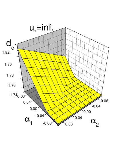
Figure 1: (Left) The scaling regimes of the model in the $\varepsilon-\eta$ plane. The region FPI corresponds to the trivial rapid-change limit: $g^{*}/u^{*}=0,1/u^{*}=0$. The region FPII corresponds to the the non-trivial rapid change limit: $g^{*}/u^{*}>0,1/u^{*}=0$. The region FPIII corresponds the trivial ”frozen” limit: $g^{*}=0,u^{*}=0$. The region FPIV is related to the non-trivial ”frozen” limit: $g^{*}>0,u^{*}=0$. In the end, the line $\varepsilon=\eta$ (FPV) corresponds to the more interesting scaling regime with $g^{*}>0,0<u^{*}<\infty$. (Right) Dependence of the borderline dimension $d_{c}$ on weak anisotropy parameters $\alpha_{1,2}$ in the Kraichnan limit of the model: $u_{*}\rightarrow\infty$.

The RG analysis leads to the conclusion that possible scaling regimes are given by the IR stable fixed points of the corresponding RG equations [5, 6, 7]. The fixed points of the RG equations can be determined in two ways: First, they are determined by the corresponding system of RG differential equations (they are know as the flow equations or Gell-Mann-Low equations), or, second, they can be found from the requirement that all the so-called beta functions of the model vanish and the IR stability of the fixed point is given by the requirement that all the eigenvalues of the matrix of the first derivatives $\Omega_{ij}=\partial\beta_{i}/\partial C_{k}$ must have positive real parts, where $\beta_{i}$ denotes the full set of beta functions and $C_{k}$ is the full set of charges of the model. In the case when uniaxial anisotropy is strong (nonrestricted), only the first possibility is suitable. It was briefly discussed in [15] where the corresponding analysis of the scaling regimes was done. In what follows, we shall concentrate on the weak anisotropy limit to better understand the situation. In this case, the second possibility leads to the result, i.e., the possible fixed points are given by the following system of equations

$$\beta_{g}(g_{*},u_{*},\chi_{i*},\alpha_{j},d,\varepsilon,\eta)=\beta_{u}(g_{*},u_{*},\chi_{i*},\alpha_{j},d,\varepsilon,\eta)=\beta_{\chi_{i}}(g_{*},u_{*},\chi_{i*},\alpha_{j},d,\varepsilon,\eta)=0,$$ (8)

for $i=1,2,3;j=1,2$, where each variable with the star denotes the corresponding fixed point value of the variable and all beta functions are linear functions of all quantities related to anisotropy, namely, $\alpha_{1},\alpha_{2},$ and $\chi_{i}$, $i=1,2,3$. The explicit form of the beta functions is as follows

$$\beta_{g}=g(-2\varepsilon+2\gamma_{1}),\quad\beta_{u}=u(-\eta+\gamma_{1}),\quad\beta_{\chi_{i}}=\chi_{i}(\gamma_{1}-\gamma_{i+1}),\quad i=1,2,3,$$ (9)

where, in the limit of weak anisotropy, the so-called gamma functions $\gamma_{i},i=1,2,3,4$ have the following explicit form

$$\gamma_{i+1}=-\frac{g}{2\chi_{i}}\frac{S_{d}}{(2\pi)^{d}}\frac{{\cal K}_{i+1}}{d(d+2)(d+4)(d+6)(1+u)^{2}},\quad i=0,1,2,3\,$$ (10)

where we define $\chi_{0}=1$, $S_{d}=2\pi^{d/2}/\Gamma(d/2)$ is the $d-$dimensional sphere, and the coefficients ${\cal K}_{i},i=1,2,3,4$ are given as follows

$${\cal K}_{1} = -(\alpha_{2}(3+d)(6+d)(1+u)+\alpha_{1}(6+d)(1+d(4+d))(1+u)-3(24+2\chi_{1}+6\chi_{2}+5\chi_{3}+24u)$$

$$+d(-30-25\chi_{1}-9\chi_{2}-3\chi_{3}-30u+d(21+10d+d^{2}-(10+d)\chi_{1}-\chi_{2}+(3+d)(7+d)u)))$$

$${\cal K}_{2} = -2(6+d)((3+d)\chi_{1}+\chi_{2})+12\chi_{3}-2\alpha_{1}(3+d)(6+d)(1+u)$$

$$+\alpha_{2}(6+d)(-10+d(-6+d(3+d)))(1+u)\,,$$

$${\cal K}_{3} = (6+d)(-2(3+d)\chi_{1}+(-10+d(-6+d(3+d)))\chi_{2})$$

$$+(-24+d(-8+d(5+d)))\chi_{3}+2\alpha_{2}(6+d)(1+u)+2\alpha_{1}(3+d)(6+d)(1+u)\,,$$

$${\cal K}_{4} = -2d(d+4)\chi_{3}\,.$$

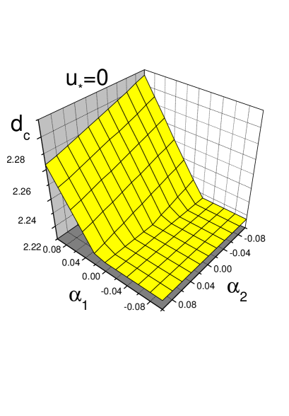
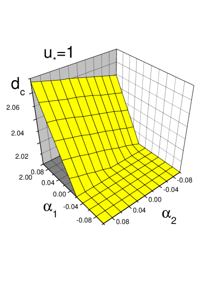
Figure 2: Dependence of the borderline dimension $d_{c}$ on weak anisotropy parameters $\alpha_{1,2}$ in the case of the so-called frozen limit of the model: $u_{*}=0$, and in the case with finite value: $u_{*}=1$.

Thus, possible fixed points are found as solutions of the system of algebraic equations (8) and their IR stability is determined by the positive real parts of the eigenvalues of the matrix $\Omega=\{\Omega_{ik}\}$. First of all, we have found all possible IR fixed points which correspond to the possible scaling regimes and we have analyzed the regions of their IR stability in the $\varepsilon-\eta$ plane. The results of this analysis are shown in Fig. 1(Left), where it is shown that the model exhibits five different scaling regimes (two for rapid-change limit, two for so-called ”frozen” limit, and one general with nonzero $u_{*}$) (see, e.g., [14] and references therein). The same situation is also held when no restrictions on the uniaxial anisotropy is supposed [15]. Further, our interest is concentrated on the investigation of the dependence of stability of the above mentioned scaling regimes on anisotropy parameters $\alpha_{1},\alpha_{2}$ and on the dimension of the space $d$. As in the strong anisotropy case we have found the so-called borderline dimension $d_{c}$ between stable and unstable regimes as a function of anisotropy parameters $\alpha_{1},\alpha_{2}$ and parameter $u_{*}$. The results are shown in Figs. 1(Right) and 2 for different fixed point values of the parameter $u$. The assumption of linearity of beta functions as a functions of anisotropy parameters leads to the fact that the borderline surface $d_{c}=d_{c}(\alpha_{1},\alpha_{2})$ consists of two intersecting planes. One of them is related to the condition $g_{*}>0$ and the second surface is related to the condition to have all real parts of eigenvalues of the matrix of the first derivatives positive. One can see that the presence of small-scale anisotropy leads to the violation of the stability of the corresponding scaling regimes below $d_{c}\in[2,3]$ for appropriate values of anisotropy parameters. But from the point of view of further investigation of anomalous scaling the most important conclusion is that all the three-dimensional scaling regimes remain stable under influence of small-scale uniaxial anisotropy.

Conclusions

In present paper we have studied the influence of weak uniaxial small-scale anisotropy on the stability of the scaling regimes in the model of a passive vector advected by given stochastic environment with finite time correlations by means of the field theoretic RG. The system exhibits five different scaling regimes. Their IR stability is related to the values of the parameters $\varepsilon$ and $\eta$. Besides, the stability of all scaling regimes is influenced by presence of small-scale anisotropy which is demonstrated in the existence of the so-called borderline dimension $d_{c}$ which is a function of the anisotropy parameters. The $d_{c}$ is defined as dimension above which the corresponding scaling regime is stable and below which the stability of the regime is destroyed. We have calculated the borderline dimension in the case when anisotropy parameters are close to zero. The assumption of linearity of beta functions as a functions of anisotropy parameters leads to the fact that the borderline surface $d_{c}=d_{c}(\alpha_{1},\alpha_{2})$ consists of two intersecting planes. All the calculations have been done at the one-loop level. The results will be used in the further investigations of the anomalous scaling of the model.

ACKNOWLEDGEMENTS — It is a pleasure to thank the Organizing Committee of the STM-2006 for kind hospitality. The work was supported in part by VEGA grant 6193 of Slovak Academy of Sciences, and by Science and Technology Assistance Agency under contract No. APVT-51-027904.

References

- [1] A.S. Monin, A.M. Yaglom, Statistical Fluid Mechanics, Vol. 2, MIT Press, Cambridge, MA, 1975.
- [2] U. Frisch, Turbulence: The Legacy of A.N. Kolmogorov, Cambridge University Press, Cambridge, 1995.
- [3] G. Falkovich, K. Gawȩdzki, M. Vergassola, Rev. Mod. Phys. 73 (2001) 913.
- [4] J. Zinn-Justin, Quantum Field Theory and Critical Phenomena (Clarendon, Oxford, 1989).
- [5] A.N. Vasil’ev, Quantum-Field Renormalization Group in the Theory of Critical Phenomena and Stochastic Dynamics, St. Petersburg: St. Petersburg Institute of Nuclear Physics, 1998 [in Russian; English translation: Gordon & Breach, 2004].
- [6] L. Ts. Adzhemyan, N. V. Antonov, and A. N. Vasil’ev, Usp. Fiz. Nauk 166 (1996) 1257 [Phys. Usp. 39 (1996) 1193].
- [7] L.Ts. Adzhemyan, N.V. Antonov, and A.N. Vasil’ev, The Field Theoretic Renormalization Group in Fully Developed Turbulence, London, Gordon Breach, 1999.
- [8] L.Ts. Adzhemyan, N.V. Antonov, and A.N. Vasil’ev, Phys. Rev. E58 (1998) 1823.
- [9] R.H. Kraichnan, Phys. Fluids 11 (1968) 945.
- [10] N.V. Antonov, J. Phys. A: Math. Gen. 39 (2006) 7825.
- [11] N. V. Antonov, A. Lanotte, and A. Mazzino, Phys. Rev. E 61, 6586 (2000); N. V. Antonov, J. Honkonen, A. Mazzino, and P. Muratore-Ginanneschi, ibid. 62 (2000) R5891.
- [12] L. Ts. Adzhemyan, N. V. Antonov, and A. V. Runov, Phys. Rev. E 64 (2001) 046310.
- [13] M. Hnatic, M. Jurcisin, A. Mazzino, S. Sprinc, acta phys. slov. 52 (2002) 559; M. Hnatic, J. Honkonen, M. Jurcisin, A. Mazzino, and S. Sprinc, Phys. Rev. E 71 (2005) 066312.
- [14] N.V. Antonov, M. Hnatic, J. Honkonen, and M. Jurcisin, Phys. Rev. E 68 (2003) 046306.
- [15] E. Jurcisinova, M. Jurcisin, R. Remecky, and M. Scholtz, Numerical Investigation of Scaling Regimes in a Model of Anisotropically Advected Vector Field, nlin.CD/0609067.
- [16] S.V. Novikov, J. Phys. A: Math. Gen. 39 (2006) 8133.