Quantum mushroom billiards

Abstract

We report the first large-scale statistical study of very high-lying eigenmodes (quantum states) of the mushroom billiard proposed by L. Bunimovich in this journal, 11, 802 (2001). The phase space of this mixed system is unusual in that it has a single regular region and a single chaotic region, and no KAM hierarchy. We verify Percival’s conjecture to high accuracy ($1.7\%$). We propose a model for dynamical tunneling and show that it predicts well the chaotic components of predominantly-regular modes. Our model explains our observed density of such superpositions dying as $E^{-1/3}$ ($E$ is the eigenvalue). We compare eigenvalue spacing distributions against Random Matrix Theory expectations, using $16000$ odd modes (an order of magnitude more than any existing study). We outline new variants of mesh-free boundary collocation methods which enable us to achieve high accuracy and such high mode numbers orders of magnitude faster than with competing methods.

Quantum chaos is the study of the quantum (wave) properties of Hamiltonian systems whose classical (ray) dynamics is chaotic. Billiards are some of the simplest and most studied examples; physically their wave analogs are vibrating membranes, quantum, electromagnetic, or acoustic cavities. They continue to provide a wealth of theoretical challenges. In particular ‘mixed’ systems, where ray phase space has both regular and chaotic regions (the generic case), are difficult to analyse. Six years ago Bunimovich described Bunimovich (2001) a mushroom billiard with simple mixed dynamics free of the usual island hierarchies of Kolmogorov-Arnold-Moser (KAM). He concluded by anticipating the growth of “quantum mushrooms”: it is this gardening task that we achieve here, by developing advanced numerical methods to collect an unprecedented large number $n$ of eigenmodes (much higher than competing numerics de Mezenes et al. (2007) or microwave studies Dietz et al. (2007)). Since uncertainties scale as $n^{-1/2}$, a large $n$ is vital for accurate spectral statistics and for studying the semiclassical (high eigenvalue) limit. We address three main issues. i) The conjecture of Percival Percival (1973) that semiclassically modes live exclusively in invariant (regular or chaotic) regions, and occur in proportion to the phase space volumes. ii) The mechanism for dynamical tunneling, or quantum coupling between classically-isolated phase space regions. iii) The distribution of spacings of nearest-neighbor eigenvalues, about which recent questions have been raised Dietz et al. (2007). We show many pictures of modes, including the boundary phase space (the so-called Husimi function).

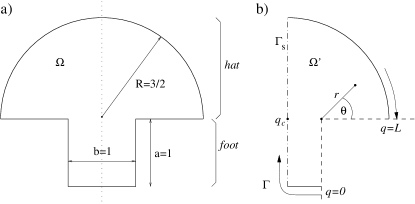
Figure 1: a) Mushroom billiard $\Omega$ used in this work. The dotted line shows the reflection symmetry. b) Desymmetrized half-mushroom ${\Omega^{\prime}}$ used for mode calculation, and polar coordinates. Dashed lines meeting at this corner are zeros enforced by basis functions. The remaining part of ${\partial\Omega^{\prime}}$ is $\Gamma$, comprising two pieces: Dirichlet boundary conditions on the parts shown as solid, while boundary conditions vary (see text) on the dash-dotted vertical line $\Gamma_{s}$. Boundary coordinate $q\in[0,L]$ parametrizes $\Gamma$.

I Introduction

The nature of eigenfunctions of linear partial differential operators in the short wavelength, or semiclassical, limit remains a key open problem which continues to engage mathematicians and physicists alike. When the operator is the quantization of a classical Hamiltonian dynamical system, the behavior of eigenfunctions depends on the class of dynamics. In particular, hyperbolic dynamics (exponential sensitivity to initial conditions, or chaos) leads to irregular eigenfunctions, the study of which forms the heart of a field known as ‘quantum chaos’ Gutzwiller (1990) or ‘quantum ergodicity’ De Bièvre (2001); Zelditch (2006). The planar billiard, or particle undergoing elastic reflection in a cavity $\Omega\subset\mathbb{R}^{2}$, is one of the simplest examples. Billiards exhibit a menagerie of dynamical classes Sinaĭ (1970); Bunimovich (1991); Sinaĭ (2004) ranging from complete integrability (ellipses and rectangles) to complete ergodicity (e.g. Sinai billiard). Bunimovich introduced the ‘mushroom’ billiard Bunimovich (2001); Porter and Lansel (2006) with the novelty of a well-understood divided phase-space comprising a single integrable (KAM) region and a single ergodic region . As seen in Fig. 1a, the mushroom is the union of a half-disk (the ‘hat’) and a rectangle (the ‘foot’); only trajectories reaching the foot are chaotic. The simplicity of its phase space has allowed analysis of phenomena such as ‘stickiness’ (power-law decay of correlations) in the ergodic region Altmann et al. (2005, 2006).

The quantum-mechanical analog of billiards is the spectral problem of the Laplacian in $\Omega$ with homogeneous boundary conditions (BCs). Choosing Dirichlet BCs (and units such that $\hbar=2m=1$) we have

$$-\Delta\phi_{j} = E_{j}\phi_{j}\qquad\mbox{in}\;\Omega,$$ (1)

$$\phi_{j} = 0\qquad\quad\mbox{on}\;{\partial\Omega}.$$ (2)

This ‘drum problem’ has a wealth of applications throughout physics and engineering Kuttler and Sigillito (1984). Eigenfunctions (or eigenmodes, modes) $\phi_{j}$ may be chosen real-valued and orthonormalized, $\langle\phi_{i},\phi_{j}\rangle\;:=\;\int_{\Omega}\phi_{i}({\mathbf{r}})\phi_{j}({\mathbf{r}}){d{\mathbf{r}}}\;=\;\delta_{ij}$, where ${d{\mathbf{r}}}:=dxdy$ is the usual area element. ‘Energy’ eigenvalues $E_{1}<E_{2}\leq E_{3}\leq\cdots\to\infty$ may be written $E_{j}=k_{j}^{2}$, where the (eigen)wavenumber $k_{j}$ is $2\pi$ divided by the wavelength.

Traditional numerical methods to compute eigenvalues and modes employ finite differences or finite elements (FEM). They handle geometric complexity well but have two major flaws: i) it is very cumbersome to achieve high convergence rates and high accuracy, and ii) since several nodes are needed per wavelength they scale poorly as the eigenvalue $E$ grows, requiring of order $E$ degrees of freedom (e.g. for the mushroom deMenezes et. al. de Menezes et al. (2007) appear limited to $j<400$). The numerical difficulty is highlighted by the fact that analog computation using microwave cavities is still popular in awkward geometries Dhar et al. (2003); Dietz et al. (2007).

In contrast we use boundary-based methods, as explained in Sec. II. These i) achieve spectral accuracy, allowing eigenvalue computations approaching machine precision as exhibited for low-lying modes in Sec. III, and ii) require only of order $E^{1/2}$ degrees of freedom (with prefactor smaller than boundary integral methods Bäcker (2003)). Furthermore at high $E$ we use an accelerated variant, the scaling method Vergini and Saraceno (1995); Barnett (2000, 2006), which results in another factor of order $E^{1/2}$ in efficiency. These improvements allow us to find large numbers of modes up to $j\sim 10^{5}$; in Sec. IV we show such modes along with their Husimi (microlocal) representations on the boundary. Visualization of modes can be an important tool, e.g. in the discovery of scars Heller (1984).

We are motivated by a growing interest in quantum ergodicity Lindenstrauss (2006); Faure et al. (2003). For purely ergodic billiards, the Quantum Ergodicity Theorem Schnirelman (1974); Colin de Verdière (1985); Zelditch (1987); Zelditch and Zworski (1996) (QET) states that in the $E\to\infty$ limit almost all modes become equidistributed (in coordinate space, and on the boundary phase space Hassell and Zelditch (2004); Bäcker et al. (2004)). However no such theorem exists for mixed billiards, thus numerical studies are vital. It is a long-standing conjecture of Percival Percival (1973) that for mixed systems, modes tend to localize to one or another invariant region of phase space, with occurence in proportion to the phase space volumes, and that those in ergodic regions are equidistributed. (This has been tested in a smooth billiard Carlo et al. (1998), and recently proved for certain piecewise linear quantum maps Marklof and O’Keefe (2005)). We test the conjecture via a matrix element (10) sensitive to the boundary (for numerical efficiency); we then can categorize (almost all) modes as regular or ergodic. We address two issues which have also been raised by recent microwave experiments in the mushroom Dietz et al. (2007). i) The mechanism for dynamical tunneling Davis and Heller (1981) is unknown (although it has been studied in KAM mixed billiards Frischat and Doron (1998)). In Sec. V we propose and test a simple model for coupling strength (related to Bäcker et al. (2007)) which predicts observed features of matrix element distributions. ii) The level-spacing distribution, conjectured to be a universal feature Gutzwiller (1990); Bohigas (1991), is studied in Sec. VI, where we also examine spacing distributions for regular and ergodic subsets of modes. Note that we use an order of magnitude more modes than any existing experiment or study. Finally we draw conclusions in Sec. VII.

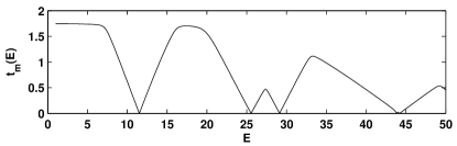
Figure 2: The tension $t_{m}(E)$ plotted as a function of trial eigenvalue parameter $E$, for the half-mushroom with Dirichlet boundary conditions. The minima indicate the eigenvalues of this domain. Close to $E=44$ there is a cluster of two eigenvalues.

II Numerical methods

In this section we outline the numerical methods that make our investigation possible; the reader purely interested in results may skip to Sec. III.

II.1 The Method of Particular Solutions

Our set of basis functions, or particular solutions, $\{\xi_{n}({\mathbf{r}})\}_{n=1\cdots N}$ satisfy $-\Delta\xi_{n}=E\xi_{n}$ at some trial eigenvalue parameter $E$, but do not individually satisfy (2). The goal is now to find values of $E$ such that there exists nontrivial linear combinations $x_{1}\xi_{1}+x_{2}\xi_{2}+\dots+x_{N}\xi_{N}$, which are small on the boundary. These are then hopefully good approximations for an eigenfunction.

Let us make this precise. We define the space $\mathcal{H}(E)$ of trial functions at a given parameter $E$ as

$$\mathcal{H}(E)=\text{Span}\{\xi_{1},\dots,\xi_{N}\}.$$

If we denote by $\|u\|_{\partial\Omega}$ and $\|u\|_{\Omega}$ the standard $L^{2}$-norm of a trial function $u\in\mathcal{H}(E)$ on the boundary ${\partial\Omega}$ and in the interior $\Omega$ we can define the normalized boundary error (also called the tension) as

$$t[u]:=\frac{\|u\|_{\partial\Omega}}{\|u\|_{\Omega}}$$ (3)

It is immediately clear that $t[u]=0$ for $u\in\mathcal{H}(E)$ if and only if $u$ is an eigenfunction and $E$ the corresponding eigenvalue on the domain $\Omega$. However, in practice we will rarely achieve exactly $t[u]=0$. We therefore define the smallest achievable error as $t_{m}(E):=\min_{u\in\mathcal{H}(E)}t[u]$. This value gives us directly a measure for the error of an eigenvalue approximation $E$, namely there exists an eigenvalue $E_{j}$ such that

$$\frac{|E-E_{j}|}{E_{j}}\leq Ct_{m}(E),$$ (4)

where $C$ is an $O(1)$ constant that only depends on the domain $\Omega$. This result is a consequence of error bounds of Moler and Payne Moler and Payne (1968); Kuttler and Sigillito (1978). Hence, by searching in $E$ for minima of $t_{m}(E)$ we find approximate eigenvalues with relative error given by a constant times $t_{m}(E)$. Fig. 2 shows such a plot of $t_{m}(E)$ for our mushroom domain.

The implementation of this Method of Particular Solutions (MPS) depends on i) basis set choice, and ii) how to evaluate $t_{m}(E)$. The former we address in the next section. The latter requires a set of quadrature points $\{{\mathbf{y}}_{i}\}_{i=1\cdots M}$ on which to approximate the boundary integral $||u||_{{\partial\Omega}}$. One must take into account that Helmholtz basis sets tend to be ill-conditioned, that is, the $M\times N$ matrix $A$ with entries $A_{in}:=\xi_{n}({\mathbf{y}}_{i})$ becomes numerically rank-deficient for desirable choices of $N$. The tension $t_{m}(E)$ can then be given by the square-root of the lowest generalized eigenvalue of the matrix pair $(A^{T}A,B^{T}B)$, or by the lowest generalized singular value of the pair $(A,B)$, where $B$ is identical to $A$ except with the replacement of $\{{\mathbf{y}}_{i}\}$ by interior points Kuttler and Sigillito (1984); Barnett (2000, ). These different approaches are discussed in Betcke (2006). Here, we use the generalized singular value implementation from Betcke (2006), which is highly accurate and numerically stable. We note that these methods are related to, but improve upon, the plane wave method of Heller Heller (1991).

II.2 Choice of basis functions

In order to obtain accurate eigenvalue and eigenfunction approximations from the MPS it is necessary to choose the right set of basis functions. In this section we propose a basis set that leads to exponential convergence, i.e. errors which scale as $e^{-cN}$ for some $c>0$, as $N$ the number of basis functions grows.

To achieve this rate we first desymmetrize the problem. The mushroom shape $\Omega$ is symmetric about a straight line going vertically through the center of the domain (see Fig. 1). All eigenmodes are either odd or even symmetric with respect to this axis. Hence, it is sufficient to consider only the right half, ${\Omega^{\prime}}$. The odd modes are obtained by imposing zero Dirichlet boundary conditions everywhere on the boundary ${\partial\Omega^{\prime}}$ of the half mushroom. The even modes are obtained by imposing zero Neumann conditions on the symmetry axis $\Gamma_{s}$ and zero Dirichlet conditions on the rest of ${\partial\Omega^{\prime}}$.

Eigenfunctions of the Laplacian are analytic everywhere inside a domain except possibly at the boundary Garabedian (1964). Eigenfunctions can be analytically extended by reflection at corners whose interior angle is an integer fraction of $\pi$ Kuttler and Sigillito (1984). The only singularity appears at the reentrant corner with angle $3\pi/2$ (where dashed lines meet in Fig. 1b). Close to this corner any eigenfunction $\phi_{j}$ can be expanded into a convergent series of Fourier-Bessel functions of the form

$$\phi_{j}(r,\theta)=\sum_{n=1}^{\infty}a_{k}J_{\frac{2n}{3}}(k_{j}r)\sin\frac{2n}{3}\theta,$$ (5)

where the polar coordinates $(r,\theta)$ are chosen as in Fig. 1b. The function $J_{\alpha}$ is the Bessel function of the first kind of order $\alpha$.

The expansion (5) suggests that the basis set $\xi_{n}:=J_{\frac{2n}{3}}(kr)\sin\frac{2n}{3}\theta$, where $k^{2}=E$, might be a good choice since these functions capture the singularity at the reentrant corner and automatically satisfy the zero boundary conditions on the segments adjacent to this corner (dashed lines in Fig. 1b). Hence, we only need to minimize the error on the remaining boundary $\Gamma$ which excludes these segments. The boundary coordinate $q\in[0,L]$ parametrizes $\Gamma$; its arc length is $L=3(1+\pi/4)$. This Fourier-Bessel basis originates with Fox, Henrici and Moler Fox et al. (1967) for the L-shaped domain; we believe it is new in quantum physics. In Betcke and Trefethen (2005) the convergence properties of this basis set are investigated and it is shown that for modes with at most one corner singularity the rate of convergence is exponential. Indeed, in practice we find $t_{m}(E_{1})=O(e^{-cN})$ for some $c>0$ as the number $N$ of basis functions grows. Hence, for the minimum $\hat{E}$ of $t_{m}(E)$ in an interval containing $E_{1}$ it follows from (4) that

$$\frac{|\hat{E}-E_{1}|}{E_{1}}\leq Ct_{m}(\hat{E})\leq Ct_{m}(E_{1})=O(e^{-cN}),$$

which shows the exponential convergence of the eigenvalue approximations $\hat{E}$ to $E_{1}$ for growing $N$.

a) 
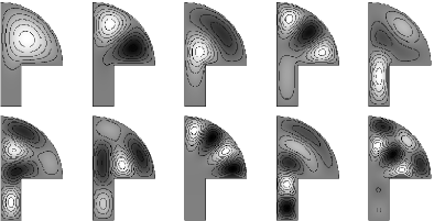
b) 

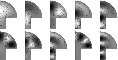
Figure 3: The first $10$ odd (a) and even (b) modes of the mushroom shape, shown as density plots. Eigenvalue increases rightwards from the top left. White corresponds to positive and black to negative values.

II.3 Scaling method at high eigenvalue

For all odd modes apart from the lowest few we used an accelerated MPS variant, the scaling method Vergini and Saraceno (1995); Barnett (2000, 2006), using the same basis as above (to our knowledge the scaling method has not been combined with a re-entrant corner-adapted basis before now). Given a center wavenumber $k_{0}$ and interval half-width $\Delta k$, the scaling method finds all modes $\phi_{j}$ with $k_{j}\in[k_{0}-\Delta k,k_{0}+\Delta k]$. This is carried out by solving a single indefinite generalized eigenvalue problem involving a pair of matrices of the type $A^{T}A$ discussed above. The ‘scaling’ requires a choice of origin; for technical reasons we are forced to choose the singular corner. Approximations to eigenvalues lying in the interval are related to the matrix generalized eigenvalues, and the modes to the eigenvectors. The errors grow Barnett (2000) as $|k_{j}-k_{0}|^{3}$, thus the interval width is determined by the accuracy desired; we used $\Delta k=0.1$ which ensured that $t_{m}(E)$ errors associated with the modes rarely exceeded $3\times 10^{-4}$. Since the search for minima required by the MPS has been avoided, and on average $O(k)$ modes live in each interval, efficiency per mode is thus $O(k)=O(E^{1/2})$ greater than the MPS. By choosing a sequence of center wavenumbers $k_{0}$ separated by $2\Delta k$, all modes in a large interval may be computed. Rather than determine the basis size $N$ by a convergence criterion as in Sec. II.2, for $E>10^{3}$ we use the Bessel function asymptotics: for large order $J_{\alpha}(x)$ becomes exponentially small for $x/\alpha<1$ (the turning point is $x=\alpha$). Equating the largest argument $kR$ (with $R=3/2$) with the largest order $2N/3$ gives our semiclassical basis size $N\approx 9k/4=O(E^{1/2})$.

We are confident that the scaling method finds all odd modes in a desired eigenvalue window. For instance we compute all 16061 odd symmetry modes with $k_{j}<300$, using 1500 applications of the scaling method (at $k_{0}=0.1,0.3,\ldots,299.9$). This computation takes roughly 2 days of CPU time . We verify in Fig. 5 that there is zero mean fluctuation in the difference between the (odd) level-counting function $N(k):=\#\{j:k_{j}\leq k\}$ and the first two terms of Weyl’s law Gutzwiller (1990),

$$N_{\mbox{\tiny Weyl}}(k)=\frac{\operatorname{vol}({\Omega^{\prime}})}{4\pi}k^{2}-\frac{|{\partial\Omega^{\prime}}|}{4\pi}k,$$ (6)

where $|{\partial\Omega^{\prime}}|$ is the full perimeter of the half mushroom domain. Note that there is no known variant of the scaling method that can handle Neumann or mixed BCs, hence we are restricted to odd modes. It is interesting that the method is still not completely understood from the numerical analysis standpoint Vergini and Saraceno (1995); Barnett (2000, 2006).

In applying the scaling method to the mushroom, the vast majority of computation time involves evaluating Bessel functions $J_{\alpha}(x)$ for large non-integral $\alpha$ and large $x$. This is especially true for producing 2D spatial plots of modes as in Fig. 8, for which of order $10^{9}$ evaluations are needed (1 hr CPU time). We currently use independent calls to the GSL library M. Galassi et al. for each $J_{\alpha}(x)$ evaluation. This is quite slow, taking between 0.2 and 50 $\mu$s per call, with the slowest being in the region $\alpha<50$, $10^{2}<x<10^{3}$. However, we note that Steed’s method Barnett et al. (1974); Press et al. (2002), which is what GSL uses in this slow region, is especially fast at evaluating sequences $J_{\alpha}(x),J_{\alpha-1}(x),J_{\alpha-2}(x),\ldots$, and that since $\alpha$ is a multiple of a rational with denominator 3, only 3 such sequences would be needed to evaluate all basis functions $\{\xi_{m}({\mathbf{r}})\}_{m=1\cdots M}$ at a given location ${\mathbf{r}}$. We anticipate at least an order of magnitude speed gain could be achieved this way.

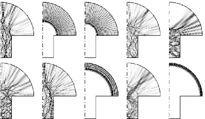
Figure 4: The 10 odd modes of the mushroom whose eigenwavenumbers lie in the range $90<k_{j}<90.35$, at mode number about $j\approx 1430$. Intensity $|\phi_{j}|^{2}$ is shown with zero white and larger values darker.

a) $j$ $E_{j}$ 1 11.50790898 2 25.55015254 3 29.12467610 4 43.85698300 5 44.20899253 6 53.05259777 7 55.20011630 8 66.42332921 9 69.22576822 10 82.01093712     b) $j$ $E_{j}$ 1 5.497868889 2 13.36396253 3 18.06778679 4 20.80579368 5 32.58992604 6 34.19488964 7 41.91198264 8 47.37567140 9 54.62497098 10 65.18713235

Table 1: Tables of a) lowest 10 odd and b) lowest 10 even eigenvalues of the mushroom. All digits shown are believed to be correct.

III Low eigenvalue modes

In this section we present highly-accurate results for the first few even and odd modes. Odd modes are obtained by solving the eigenvalue problem with zero Dirichlet boundary conditions on the half mushroom from Fig. 1b, using the MPS, by locating minima in the tension function of Fig. 2. In Table 1a the eigenvalues are listed to at least 10 significant digits, and in Fig. 3a the corresponding modes are plotted. We emphasize that it is the exponential convergence of our basis that makes such high accuracies a simple task.

For even modes we impose Neumann BCs on $\Gamma_{s}$ and Dirichlet BCs on the remaining part of $\Gamma$. This was achieved in the MPS by modifying the tension function (3) to read

$$t[u]:=\frac{\left(\|\partial_{n}u\|_{\Gamma_{s}}^{2}+\|u\|_{\Gamma\backslash\Gamma_{s}}^{2}\right)^{1/2}}{\|u\|_{\Omega^{\prime}}}$$ (7)

where the normal derivative operator on the boundary is $\partial_{n}:={\mathbf{n}}\cdot\nabla$, the unit normal vector being ${\mathbf{n}}$. Table 1b, gives the smallest $10$ even modes on the mushroom billiard, and the corresponding modes are plotted in Fig. 3b.

Although we are far below the semiclassical regime we already see properties of the underlying classical dynamical system. For example, the $8^{th}$ odd and the $6^{th}$ even mode live along a caustic and therefore show features of the classically integrable phase space while the $7^{th}$ odd and $10^{th}$ even mode already shows features of the classically ergodic phase space. For comparison, in Fig. 4 we show some odd modes with intermediate eigenvalues of order $10^{4}$ (odd mode number of order $10^{3}$), a similar quantum number to that measured in a microwave cavity by Dietz et. al. Dietz et al. (2007). As these authors noted, modes at this energy usually live in either the integrable or to the ergodic regions of phase space; we pursue this in detail in Sec. V.

Figure 5: Difference between the mode counting function $N(k)$ and the two-term Weyl’s prediction $N_{\mbox{\tiny Weyl}}(k)$ defined by (6), for the 16061 odd-symmetric eigenvalues with $k_{j}<300$.

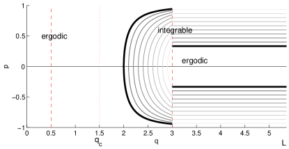
Figure 6: Poincaré surface of section (PSOS), that is, the classical phase space in boundary coordinates $q$ (as shown in Fig. 1b) and $p$ (sin of incidence angle). Vertical dashed lines shows location of corners. The vertical dotted line shows location of $q_{c}$ the focal point of the hat. The dark line shows the border of integrable phase space; note that $q=2$ corresponds to the smallest possible caustic for integrable phase space. Families of orbits defined by constant angular momentum are shown by lines in the integrable region. Note that they exchange vertical ordering at the corner, as indicated by their grayscale color labeling.

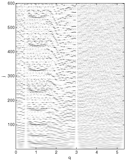
Figure 7: Intensity of boundary normal-derivative functions $|{\partial_{n}\phi_{j}}(q)/k_{j}|^{2}$, plotted vs boundary coordinate $q$ on the horizontal axis and odd mode number $j\in[1,600]$ on the vertical. The density plot shows white as zero, and larger values darker.

IV Boundary and Husimi functions

We choose a Poincaré surface of section (PSOS) Gutzwiller (1990) defined by Birkhoff coordinates $(q,p)\in\Gamma\times[-1,1]=:Z$, where $q$ is the boundary location as before (see Fig. 1b) and $p$ the tangential velocity component, in the clockwise sense, for a unit speed particle. (If the incident angle from the normal is $\theta$ then $p=\sin\theta$). The structure of this PSOS phase space is shown in Fig. 6. Our choice (which differs from that of Porter et. al. Porter and Lansel (2006)) is numerically convenient since it involves only the part of the boundary on which matching is done (Sec. II). Despite the fact that it does not cover the whole boundary ${\partial\Omega^{\prime}}$, it is a valid PSOS since all trajectories must hit $\Gamma$ within bounded time.

Integrable phase space consists of precisely the orbits which, for all time, remain in the hat Bunimovich (2001) but which never come within a distance $b/2$ from the center point $q_{c}$ . Simple geometry shows that the curved boundary between ergodic and integrable regions consists of points $(q,p)$ satisfying

$$q-q_{c}\;=\;\frac{b/2}{\sqrt{1-p^{2}}},\quad\mbox{for}\;\;p^{2}\leq p_{0}^{2}:=1-\frac{b^{2}}{4R^{2}}.$$ (8)

For our shape, $q_{c}=a+b/2=3/2$, $p_{0}^{2}=8/9$. In the domain $q\in[q_{c}+R,L]$ the boundary occurs at the lines $p=\pm b/2R=\pm 1/3$. Successive bounces that occur on $\Gamma$ are described by the PSOS billiard map $f:Z\to Z$. Any such Poincaré map is symplectic and therefore area-preserving Gutzwiller (1990).

The quantum boundary functions ${\partial_{n}\phi_{j}}(q)$ for $q\in[0,L]$ are convenient and natural representations of the modes. Note that they are not $L^{2}({\partial\Omega})$ normalized; rather they are normalized according to a geometrically-weighted $L^{2}$ boundary norm via the Rellich formula (see Rellich (1940); Barnett (2006))

$$\int_{\partial\Omega}({\mathbf{r}}\cdot{\mathbf{n}})\,|{\partial_{n}\phi_{j}}|^{2}\,dq=2E_{j},$$ (9)

where ${\mathbf{r}}(q)$ is the location of boundary point $q$ relative to an arbitrary fixed origin. Fig. 7 shows the intensities of the first 600 odd boundary functions. Features include an absence of intensity near the corners (over a region whose size scales as the wavelength). The region $3<q<L$, in which phase space is predominantly integrable, has a more uniform intensity than $0<q<2$, which is exclusively ergodic. The region $2<q<3$ is almost exclusively integrable, but is dominated by classical turning-points corresponding to caustics; these appear as dark Airy-like spots. In $1/2<q<3/2$ there are horizontal dark streaks corresponding to horizontal ‘bouncing-ball’ (BB) modes in the foot. Finally, a series of slanted dark streaks is visible for $3/2<q<2$: these interesting fringes move as a function of wavenumber and we postpone analysis to a future publication.

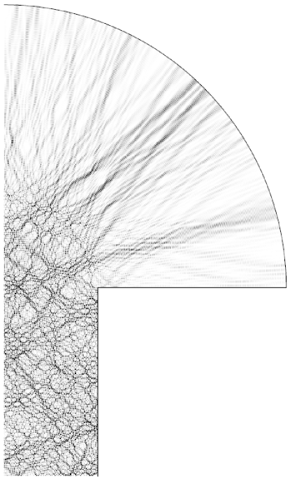
Figure 8: High-energy eigenmode with $k_{j}=499.856\cdots$, at around odd mode number $j\approx 45000$. This mode appears to live in the ergodic region.

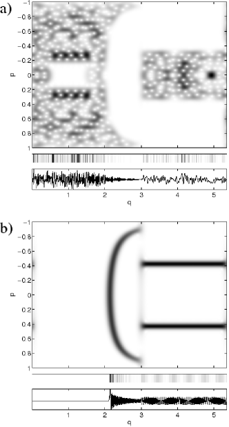
Figure 9: a) the mode of Fig. 8 Husimi distribution $H_{{\partial_{n}\phi_{j}},\sigma}(q,p)$ defined by (20) (top), density plot of $|{\partial_{n}\phi_{j}}|^{2}$ (middle), and graph of ${\partial_{n}\phi_{j}}$ (bottom). Note the $q$ coordinate is common to the three plots. b) Similar representation of the next highest mode at $k_{j}=499.858$, the 15^th in the sequence of Fig. 14, which lives in the regular region.

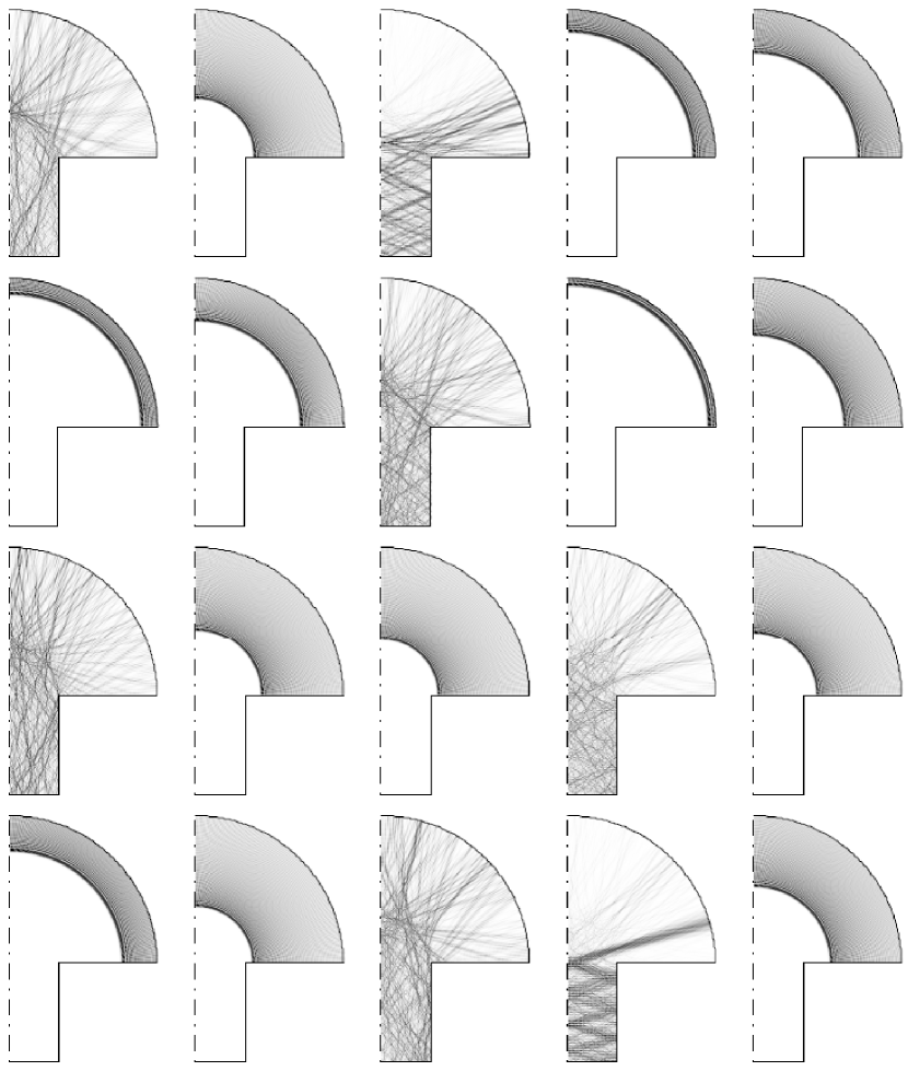
Figure 14: 20 high-eigenvalue consecutive modes, covering the range $k_{j}\in[499.800,499.869]$, with mode number $j\approx 45000$. Mode number increases horizontally from the top left. $|\phi_{j}|^{2}$ is shown with zero white and larger values darker.

In Fig. 14 we show a sequence of 20 much higher modes with consecutive eigenvalues near wavenumber $k=500$ (eigenvalue $E=2.5\times 10^{5}$). These modes are a subset of the modes produced via a single generalized matrix eigenvalue problem (of size $N\approx 1200$) using the scaling method at $k_{0}=500$. The full set of 77 modes (evaluating boundary functions) took only 20 mins CPU time. Typical tension $t_{m}(E)$ values were below $10^{-3}$. Naively applying (4) we would conclude only about 3 relative digits of accuracy on eigenvalues. However, it is possible to rigorously improve this bound by factor $O(E_{j}^{1/2})$ Barnett , giving about 6 digits.

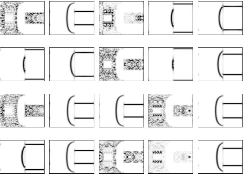
Figure 15: Husimi distributions $H_{{\partial_{n}\phi_{j}},\sigma}(q,p)$ of the 20 high-eigenvalue modes shown in Fig. 14, and in the same order. The $q$ and $p$ axes are as in Fig. 9.

Fig. 8 shows the 14th in the sequence in more detail. The corresponding boundary function is shown in Fig. 9a, along with the intensity, and its Husimi distribution. The Husimi distribution is a coherent-state projection of the mode onto the PSOS phase space (see App. A). The choice of the aspect ratio $\sigma$ is somewhat arbitrary but it is expected Heller (1984) that phase space structures have spatial scale $O(k^{-1/2})$, so we chose a scaling similar to this: with $k=500$ we used $\sigma=0.076$. By comparing to the phase space (Fig. 6) we see localization to the ergodic region. The only part of ergodic phase space not well covered contains BB modes in the foot (the white ‘box’). A scar is also visible as the 9 darkest spots: 4 pairs of spots surrounding the white box correspond to 4 bounces in the foot, and a single spot at $q\approx 5$ corresponds to a normal-incidence bounce off the circular arc. By contrast, Fig. 9b shows the boundary function of a mode living in the regular region (the 15th in Fig. 8); the energy-shell localization is clear. The full set of 20 Husimi functions is shown in Fig. 15. We remind the reader that in purely ergodic systems boundary functions obey the QET Hassell and Zelditch (2004); Bäcker et al. (2004) with almost every ${\partial_{n}\phi_{j}}/k_{j}$ tending to an invariant Husimi density of the form $C\sqrt{1-p^{2}}$. We might expect a similar result for the ergodic subset of modes in the ergodic phase space of the mushroom. However, Fig. 15 highlights that, despite being at a high mode number of roughly $4\times 10^{4}$, we are still a long way from reaching any invariant density: the 7 ergodic modes have highly non-uniform distributions.

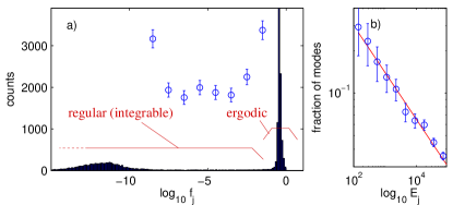
Figure 10: a) Histogram of the logarithm of $f_{j}$, the ‘foot-sensing’ matrix element (10), for the first 16061 odd modes. Errorbars show counts of $f_{j}$ lying in each decade (errors assuming independent counts), on a vertical scale magnified by a factor 15. b) Fraction of modes with $10^{-8}<f_{j}<10^{-2}$ lying in logarithmically-spaced $E_{j}$ intervals (errorbars), compared to power law $E^{-1/3}$ (solid line).

V Percival’s conjecture and dynamical tunneling

In the small set of 20 high-lying modes discussed above, Percival’s conjecture holds: modes are either regular or chaotic but not a mixture of both. We will now study this statistically with a much larger set, the first $n=16061$ odd modes corresponding to $0<k_{j}<300$. Since the PSOS phase space in $0<q<3/2$ is ergodic for all $p$, the following ‘foot-sensing’ quadratic form, or diagonal matrix element, is a good indicator of an ergodic component:

$$f_{j}:=\frac{1}{2E_{j}}\int_{0}^{3/2}({\mathbf{r}}\cdot{\mathbf{n}})\left|{\partial_{n}\phi_{j}}\right|^{2}dq,$$ (10)

where, as Fig. 1b shows, ${\mathbf{r}}\cdot{\mathbf{n}}$ takes the value 1 for $0<q<1/2$, and $1/2$ for $1/2<q<3/2$. (The weighting by ${\mathbf{r}}\cdot{\mathbf{n}}$ is chosen to mirror (9); scaling by $E_{j}$ is necessary for a well-defined semiclassical limit Hassell and Zelditch (2004); Bäcker et al. (2002)).

The observed distribution of $f_{j}$ is shown in Fig. 10a. The main feature is a cluster around $O(1)$ (we associate with ergodic modes) and a wider distribution of smaller values (predominantly regular modes). We have tested that the apparent cluster lying roughly from $10^{-14}$ to $10^{-9}$ is merely an artifact reflecting the size of numerical errors in ${\partial_{n}\phi_{j}}$: the key point is that there is a continuum of values (see errorbars in Fig. 10a) which extends from $O(1)$ down to exponentially small values. Roughly 0.75% of the total number of modes fall within each decade from $10^{-2}$ to $10^{-8}$. We believe that in the absence of numerical errors a similar distribution would extend down many tens of orders of magnitude.

Percival’s conjecture would imply that the sequence $\{f_{j}\}_{j=1\cdots\infty}$ has (for all but a set of vanishing measure) two limit points: zero (for regular modes), and some positive constant (for ergodic modes). Even though most mode numbers are large ($\sim 10^{4}$) the upper cluster still has a wide standard deviation of 0.1 (its mean is 0.39); this is in line with our recent work confirming the slow algebraic semiclassical convergence of matrix elements Barnett (2006).

We would like to test whether the relative mode frequencies of regular vs ergodic modes are in proportion to the corresponding classical phase-space volumes. We categorize modes by defining them as ‘regular’ if $f_{j}<0.1$. This choice of cutoff value is necessarily a compromise between lying below the whole ergodic peak yet capturing the full dynamic range of regular modes. This gives a fraction $\alpha_{\mbox{\tiny reg}}:=n_{\mbox{\tiny reg}}/n=7178/16061=0.4469\cdots$ of regular modes, which is only 1.7% less than the integrable phase space fraction $\mu_{\mbox{\tiny reg}}=0.4549\cdots$ (computed in App. B). Assuming that each regular mode counted arose randomly and independently due to some underlying rate (fraction of level density), we may associate a standard error of $\sqrt{n_{\mbox{\tiny reg}}(n-n_{\mbox{\tiny reg}})/n^{3}}=0.004$ with the measured fraction. Thus the discrepancy is only 2 sigma, not inconsistent with the (null) hypothesis that $\alpha_{\mbox{\tiny reg}}=\mu_{\mbox{\tiny reg}}$. To check whether this result persists semiclassically we computed a smaller set of $n=615$ high-lying modes sampled from the range $500<k_{j}<750$, up to mode number $j\approx 10^{5}$, and found $\alpha_{\mbox{\tiny reg}}=0.441\pm 0.015$, again consistent with Percival’s conjecture.

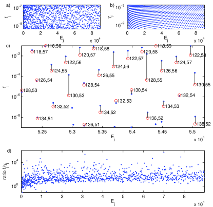
Figure 11: a) Distribution of matrix elements $f_{j}$ for regular modes, as function of eigenvalue $E_{j}$. b) Corresponding rates $\gamma_{j}$ predicted by the model in the text. c) Zoom of a), showing $f_{j}$ (dots) connected by vertical lines to best-matching values of $c\gamma_{j}$ (circles labeled by disc quantum numbers $m,n$), using constant $c=15$. d) ratio $f_{j}/\gamma_{j}$ for all matched pairs.

V.1 Results and model for dynamical tunneling

The continuum of matrix element values in Fig. 10a is a manifestation of dynamical tunneling Davis and Heller (1981), quantum coupling between regular and ergodic invariant phase space regions. This has recently been seen in mushroom microwave cavity modes Dietz et al. (2007), and these authors raised the question as to the mechanism for tunneling in this shape. We address this by proposing and numerically testing a simple such model. First we notice that the density of $\ln f_{j}$ is roughly constant (in the range $f_{h}>10^{-8}$ where numerical errors are negligible). This suggests a coupling strength which is the exponential of some uniformly-distributed quantity. We may ask whether this density is dependent on eigenvalue magnitude (energy): Fig. 10b shows that the density appears to die as $E^{-1/3}$, consistent with the expectation that all $f_{j}$ values for regular modes vanish in the semiclassical limit.

Our model is to assume that $f_{j}$ values are controlled by a matrix element $\gamma_{j}$ giving the rate of dynamical tunneling from the regular to the ergodic region. Each regular mode closely approximates an $(n,m)$-mode of the quarter disc, which are the product of angular function $(2/\sqrt{\pi})\sin m\theta$ and radial function

$$\psi_{mn}(r)=\frac{\sqrt{2}}{RJ^{\prime}_{m}(k_{mn}R)}J_{m}(k_{mn}r)$$ (11)

where $n=1,2,\ldots$ is the radial mode number and $m=2,4,\ldots$ the angular mode number, and $k_{mn}R$ is the argument of the $n^{th}$ zero of the $J_{m}$ Bessel function. Quarter-disc eigenwavenumbers are $k_{mn}$. The normalization is $\int_{0}^{R}|\psi_{mn}(r)|^{2}\,rdr=1$. A wavepacket initially launched from such a disc mode will, in the mushroom, leak into the ergodic region due to the openness of the connection into the foot. We take the rate proportional to the probability mass of $\psi_{mn}$ ‘colliding’ with the foot,

$$\gamma_{j}:=\int_{0}^{b/2}|\psi_{mn}(r)|^{2}\,rdr$$ (12)

$$=\frac{4}{[k_{mn}RJ^{\prime}_{m}(k_{mn}R)]^{2}}\sum_{l=0}^{\infty}(m+1+2l)\left|J_{m+1+2l}\left(\frac{b}{2}k_{mn}\right)\!\right|^{2}$$

where we used (Abramowitz and Stegun, 1964, Eq. 11.3.2) to rewrite the integral. This model is similar to that proposed recently by Bäcker et. al. Bäcker et al. (2007) (in our case the ‘fictitious integrable system’ is the quarter-disc). $\gamma_{j}$ is exponentially small only when the Bessel function turning point lies at radius greater than $b/2$; at eigenvalue $E$ this occurs for $b\sqrt{E}/(2m)<1$.

We compare in Fig. 11a) and b) $f_{j}$ values for regular against $\gamma_{j}$ values computed using all relevant $(m,n)$ quantum numbers for the quarter-disc. It is clear that although the densities are similar, $f_{j}$ is irregularly distributed whereas $\gamma_{j}$ values fall on a regular lattice. However, upon closer examination there is a strong correlation. We attempted to match each disc mode $(m,n)$ seen in panel b) with its corresponding mushroom mode $j$ as seen in panel a); in most of the 1051 cases there was a very clear match, with relative eigenvalue difference $|E_{j}-k_{mn}^{2}|/E_{j}<10^{-4}$ in 90% of the cases, and $|E_{j}-k_{mn}^{2}|/E_{j}<3\times 10^{-6}$ in 74% of cases. (Note that, although it is not needed for our study, it would likely be possible to improve the fraction matched using data from ${\partial_{n}\phi_{j}}$.) As shown in panel c), $f_{j}$ values are quite correlated with the $\gamma_{j}$ values of their matched mode. Note that an overall prefactor of $c=15$ was included to improve the fit. The resulting ratio $f_{j}/\gamma_{j}$ is shown in panel d), and has a spread of typically a factor $10^{2}$. Since this is much less than the spread of $10^{8}$ in the original matrix elements, this indicates that the above model is strongly predictive of dynamical tunneling strength, mode for mode. We suggest the remaining variation, and the value of $c$, might be explained by varying eigenvalue gaps (resonant tunneling) between quarter-disc and ergodic modes (such variation is discussed in Frischat and Doron (1998)), although this is an open question. Also in this simple model it is clear from the $E$-dependence in panel d) that there are algebraic prefactors that should be included in a more detailed model.

Using the model we may predict the decay $\sim E^{-1/3}$ in the density of $f_{j}$ values reported above, by returning to the sum in (12). For regular modes where $\gamma_{j}\ll 1$, the Bessel functions in the $l\geq 1$ terms have turning points successively further away from $b/2$, thus the sum may be approximated by the $l=0$ term (this has been checked numerically). We make the approximation that the turning point is close to $b/2$, that is $\varepsilon\ll 1$, where

$$\varepsilon\;:=\;1-\frac{bk_{mn}}{2m}\quad.$$ (13)

We focus on the exponentially small behavior of $\gamma_{j}$ and drop algebraic prefactors. In (12) using Debye’s asymptotics for the Bessel function (Abramowitz and Stegun, 1964, Eq. 9.3.7) and keeping leading terms for small $\varepsilon>0$ gives

$$g:=-\ln\gamma_{j}\;\approx\;(\mbox{const})+\frac{1}{2}\ln\varepsilon+\ln k_{mn}+\frac{4\sqrt{2}}{3}m\varepsilon^{3/2}.$$ (14)

(This can be interpreted as the tail of the Airy approximation to the Bessel). For fixed $\varepsilon\ll 1$ we need keep only the last term as $m\to\infty$. Fixing $m$ while increasing $n$ by 1 causes a small wavenumber change $k_{m,n+1}-k_{mn}\approx\pi/(p_{0}R)$, causing via (13) a change $\Delta\varepsilon\approx-\pi b/(2mp_{0}R)$, which in turn causes via (14) a change

$$\Delta g\;\approx\;-\pi\sqrt{2\varepsilon}/(p_{0}R)\;\approx\;-\frac{\pi}{p_{0}R}\left(\frac{3g}{2m}\right)^{1/3}~{},$$ (15)

where in the last step we expressed $\varepsilon$ in terms of the asymptotic for $g$. Realising that, for $\varepsilon\ll 1$ we have $m\approx bk_{mn}/2=b\sqrt{E}/2$, and that adjacent curves of constant $m$ in the $(E,g)$-plane are separated in $E$ by $\Delta E\approx 8\sqrt{E}/b$, gives our result, the density of points in the $(E,g)$-plane,

$$d(E,g)\;=\;\frac{1}{|\Delta g\,\Delta E|}\;\approx\;\frac{p_{0}R}{8\pi}\left(\frac{b^{4}}{3gE}\right)^{1/3}\quad.$$ (16)

Recall that Fig. 11a,b,c illustrate the $(E,g)$-plane. In Fig. 10a small dynamic range and counting statistics prevents this weak dependence of density on $g$ from being detected. However the main conclusion from (16) is that the density of $\gamma_{j}$ (and hence $f_{j}$) values lying in any fixed interval scales asymptotically as $E^{-1/3}$, in agreement with Fig. 10b.

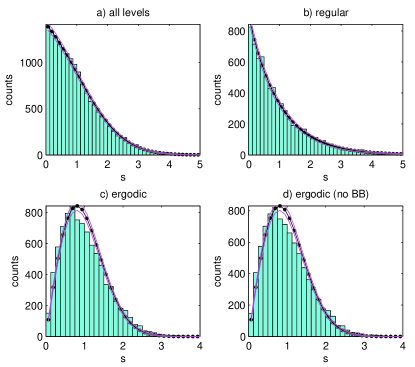
Figure 12: Nearest-neighbor spacing distributions (NNDS) $p(s)$ for the 16061 modes with $k_{j}<300$, estimated via a histogram with bins of width $\Delta s=0.125$. Data (in counts per bin) are shown by bars. Predictions are shown by dots, with $\pm 1$ standard error (solid lines above and below). a) all modes, vs Berry-Robnik formula, b) regular modes, vs Poissonian formula $e^{-s}$, c) ergodic modes including BB modes, vs Wigner’s approximate GOE formula $\frac{\pi}{2}se^{-\pi s^{2}/4}$, and d) ergodic modes with BB modes removed using the categorization in Sec. VI, vs the same.

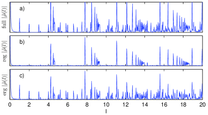
Figure 13: Absolute value of the Fourier transform $\tilde{\rho}(l)$ of the density of states $\rho(k):=\sum_{j=1}^{\infty}\delta(k-k_{j})$, vs orbit length $l$, for a) all eigenvalues lying below $k_{j}<300$, b) regular modes only, c) ergodic modes only.

VI Level spacing distribution and level density fluctuation

We show the nearest-neighbor spacing distribution (NNDS) of the complete set of the first $n=16061$ eigenvalues of odd-symmetric modes $E_{j}$ with $k_{j}<300$, in Fig. 12a. Spacings were unfolded in the standard way Bohigas (1991), thus a histogram of $s_{j}:=(E_{j+1}-E_{j})/\overline{E}$, where $\overline{E}$ is the mean level spacing, was collected. This is compared in the figure against the Berry-Robnik prediction Berry and Robnik (1984) for a mixed system with a single regular component (of phase-space fraction $\mu_{\mbox{\tiny reg}}=0.4549\cdots$) and single ergodic component. The agreement is excellent, with deviations consistent with the standard error for each bin count. In their recent work Dietz et. al. Dietz et al. (2007) claim that there is a dip in the NNDS around $s=0.7$ associated with supershell structure in the hat (two periodic orbits of close lengths). Their choice of mushroom shape differs from ours only in the foot. Our results, computed using over 16 times their number of levels, show no such dip. This suggests that their observed dip is a statistical anomaly, or that it does not carry over to the rectangular-foot mushroom and therefore is not associated with the hat.

In order to study this further we computed the partial NNDS associated with regular or ergodic modes, categorized using the method of Sec. V. Regular modes (Fig. 12b) fit the Poisson level spacing distribution well. Ergodic modes (Fig. 12c) fit Wigner’s standard approximate form for the GOE distribution reasonably well, however there are visible deviations: the data systematically favors small spacings $s<0.75$ while disfavoring intermediate spacings $0.75<s<1.6$. This can be quantified by comparing 0.392, the fraction of spacings with $s<0.75$, to 0.357, the corresponding fraction predicted using the Wigner distribution. Using the normal approximation to the binomial distribution, this discrepancy is nearly 7$\sigma$ and is thus statistically very significant (similar conclusions are reached by the standard Kolmogorov-Smirnov test for comparing distributions). We conjecture that, as with mode intensities discussed above, the discrepancy is another manifestation of slow convergence to the semiclassical limit.

One difference between our mushroom and that of Dietz et. al. is that our foot supports BB orbits and theirs does not. Therefore to eliminate this as a cause of difference, in Fig. 12d we show the ergodic NNDS with BB modes removed. Here BB modes were identified as those with $f_{j}>0.7$ but small integral on the base of the foot, namely $\int_{0}^{1/2}({\mathbf{n}}\cdot{\mathbf{r}})|{\partial_{n}\phi_{j}}|^{2}dq<0.1$; the BB subset comprises only 0.8% of the total. The difference between panels c) and d) is barely perceptible, indicating that BB modes are not a significant contribution in our setting.

Finally, in Fig. 13 we show the amplitude spectrum $\tilde{\rho}(l):=\sum_{j=1}^{n}e^{ik_{j}l}$ of the density of states, which highlights contributions from periodic orbits of length $l$. Panel a) shows all levels, while b) and c) shows the contribution only of levels categorized as either regular or ergodic, according to the above method. The periodic peaks at the integers in panel a) (and absent in b) are due to the BB mode in the foot. As expected, b) contains only the regular clusters of peaks associated with hat orbits which unfold to polygons in the disc. Each cluster of peaks has an upper limit point at multiples of $\pi R=3\pi/2$ corresponding to whispering-gallery rays. It is interesting that c) contains contributions not only from UPOs but from all the peaks of b) too.

VII Conclusion

We have presented the first known high-lying eigenmode calculations of Bunimovich’s mushroom, which has unusually simple divided phase space without KAM hierarchy. Using a basis set adapted to the re-entrant corner, the Method of Particular Solutions achieves very high accuracy for low modes, and the scaling method enables us to find high modes orders of magnitude more efficiently than any other known numerical approach, allowing the lowest $n=16061$ odd modes to be computed in reasonable time. Since statistical estimation errors scale as $1/\sqrt{n}$, we are therefore able to reach the 1% level for many quantities.

Chaotic modes and Husimi functions have been shown to be nonuniform and scarred even at mode number $\approx 45000$, evidence that the semiclassical limit is reached very slowly. Using a separation into regular vs chaotic modes, Percival’s conjecture has been verified to within 2%. A new model for dynamical tunneling (similar to that of Bäcker et. al. Bäcker et al. (2007)) has been described, and shown to predict the chaotic component of predominantly-regular modes to within a factor of roughly an order of magnitude (over a range of $10^{8}$). Its prediction (via Bessel asymptotics) that the density of occurrence of modes which are regular-chaotic superpositions dies asymptotically like $E^{-1/3}$ agrees well with the first known measurement of this density.

Our study of nearest-neighbor eigenvalue spacing finds good agreement with the Berry-Robnik distribution, and for the regular subset, good agreement with the Poisson distribution. The ergodic subset shows statistically-significant deviations from Wigner’s GOE approximation, favoring small spacings. However we find no evidence for the dip reported at $s=0.7$ by Dietz et. al. Dietz et al. (2007); recall we study over 16 times their number of modes.

This study is preliminary, and raises many interesting questions: Can our model for dynamical tunneling be refined to give agreement at the impressive level found in quantum maps Bäcker et al. (2007)? Does the ergodic level-spacing distribution eventually tend to the GOE expectation? Finally, can spectral manifestations of stickiness Altmann et al. (2005, 2006) be detected?

Appendix A Husimi transform

We define the Husimi transform Tualle and Voros (1995) of functions on $\mathbb{R}$, for convenience reviewing the coherent state formalism in dimensionless ($\hbar$-free) units. Given a width parameter (phase space aspect-ratio) $\sigma>0$, it is easy to show that the annihilation operator

$$a:=\frac{1}{\sqrt{2}}\left(\frac{q}{\sigma}+\sigma\partial_{q}\right)$$ (17)

has a kernel spanned by the $L^{2}$-normalized Gaussian $\psi_{0}(q):=(\pi\sigma^{2})^{-1/4}e^{-q^{2}/2\sigma^{2}}$. We work in $L^{2}(\mathbb{R})$, in which the hermitian adjoint of $a$ is $a^{\dagger}=(q/\sigma-\sigma\partial_{q})/\sqrt{2}$. From the commutator $[a,a^{\dagger}]=1$ it follows, $\forall z\in\mathbb{C}$, that the coherent state

$$\psi_{z}:=e^{-|z|^{2}/2}e^{za^{\dagger}}\psi_{0}$$ (18)

is an eigenfunction of $a$ with eigenvalue $z$. The fact that it is $L^{2}$-normalized requires the Hermite-Gauss normalization $\|(a^{\dagger})^{n}\psi_{0}\|_{2}^{2}=n!,\forall n\in\mathbb{N}$, which can be proved by induction. The Bargmann representation Bargmann (1961, 1967) of a function $v:\mathbb{R}\to\mathbb{C}$ is then $\langle\psi_{z},v\rangle$; the Husimi representation is its squared magnitude $H_{v,\sigma}(z):=|\langle\psi_{z},v\rangle|^{2}$. We need a more explicit form than (18). $\psi_{z}=e^{za^{\dagger}-z^{*}a}\psi_{0}$ follows by the Baker-Campbell-Hausdorff formula $e^{A+B}=e^{-[A,B]/2}e^{A}e^{B}$ for $[[A,B],A]=[[A,B],B]=0$. Applying this formula again and writing $z:=(q_{0}/\sigma+i\sigma k_{0})/\sqrt{2}$ where $q_{0},k_{0}\in\mathbb{R}$ gives

$$\psi_{z}(q)=e^{ik_{0}q_{0}/2}e^{ik_{0}q}\psi_{0}(q-q_{0}).$$ (19)

This shows that the coherent state is localized in position (around $q_{0}$) and wavenumber (around $k_{0}$), thus the Husimi is a microlocal (phase space) represention,

$$H_{v,\sigma}(q_{0},k_{0}):=\left|\int_{-\infty}^{\infty}v(q)e^{ik_{0}q}\psi_{0}(q-q_{0})dq\right|^{2}.$$ (20)

This also known as the Gabor transform or spectrogram (windowed Fourier transform), and it can be proven equal to the Wigner transform convolved by the smoothing function $\psi_{0}^{2}$. Given a normal-derivative function ${\partial_{n}\phi_{j}}$ we periodize it in order to apply the above. We also scale the wavenumber by $k_{j}$, thus the Birkhoff momentum coordinate is $p=k_{0}/k_{j}$.

Appendix B Integrable phase-space fraction

The total phase space (restricting to the unit-speed momentum shell) has volume $V_{{\mbox{\tiny tot}}}=\operatorname{vol}({\Omega^{\prime}}\times S^{1})=2\pi\operatorname{vol}{\Omega^{\prime}}=2\pi(ab/2+\pi R^{2}/4)$. Define the function $\alpha({\mathbf{r}}):=2\pi-4\sin^{-1}(b/2d({\mathbf{r}}))$, where $d({\mathbf{r}})$ is the distance from ${\mathbf{r}}$ to the center point $q_{c}$. When ${\mathbf{r}}$ is in the hat and $d({\mathbf{r}})\in[b/2,R]$, $\alpha({\mathbf{r}})$ gives the measure of the set of angles in $S^{1}$ for which orbits launched from ${\mathbf{r}}$ are integrable (i.e. never leave the annulus $d({\mathbf{r}})\in[b/2,R]$). The regular phase space volume is found by integrating $\alpha({\mathbf{r}})$ over the quarter-annulus using polar coordinates $(\rho,\phi)$:

$$V_{{\mbox{\tiny reg}}} = \int_{0}^{\pi/2}d\phi\int_{b/2}^{R}\alpha(\rho)\rho d\rho$$

$$= \frac{\pi^{2}}{2}\left(R^{2}-\frac{b^{2}}{4}\right)-2\pi\int_{b/2}^{R}\rho\sin^{-1}\frac{b}{2\rho}\,d\rho$$

$$= \pi R^{2}\left(\cos^{-1}\frac{b}{2R}\;-\;\frac{b}{2R}p_{0}\right)~{}.$$

The same result is given without calculus using the space of oriented lines in a full annulus, that is, $4V_{\mbox{\tiny reg}}=2\pi$ times the area of the segments $\{(x,y):x^{2}+y^{2}<R^{2},|y|>b/2\}$. For our parameters we get $\mu_{\mbox{\tiny reg}}:=V_{{\mbox{\tiny reg}}}/V_{{\mbox{\tiny tot}}}=0.4549\cdots$

References

- Bunimovich (2001) L. A. Bunimovich, CHAOS 11 (2001).
- de Mezenes et al. (2007) D. D. de Mezenes, M. Jar e Silva, and F. M. de Aguiar, CHAOS 17, 023116 (2007).
- Dietz et al. (2007) B. Dietz, T. Friedrich, M. Miski-Oglu, A. Richter, and S. Schäfer, Phys. Rev. E 75, 035203 (2007).
- Percival (1973) I. C. Percival, J. Phys. B pp. L229–232 (1973).
- Gutzwiller (1990) M. C. Gutzwiller, Chaos in classical and quantum mechanics, vol. 1 of Interdisciplinary Applied Mathematics (Springer-Verlag, New York, 1990).
- De Bièvre (2001) S. De Bièvre, in Second Summer School in Analysis and Mathematical Physics (Cuernavaca, 2000) (Amer. Math. Soc., Providence, RI, 2001), vol. 289 of Contemp. Math., pp. 161–218.
- Zelditch (2006) S. Zelditch, in Elsevier Encyclopedia of Mathematical Physics (Academic Press, 2006), http://arxiv.org/math-ph/0503026.
- Sinaĭ (1970) Y. G. Sinaĭ, Uspehi Mat. Nauk 25, 141 (1970).
- Bunimovich (1991) L. A. Bunimovich, CHAOS 1, 187 (1991).
- Sinaĭ (2004) Y. G. Sinaĭ, Notices Amer. Math. Soc. 51, 412 (2004).
- Porter and Lansel (2006) M. A. Porter and S. Lansel, Notices Amer. Math. Soc. 53, 334 (2006).
- Altmann et al. (2005) E. G. Altmann, A. E. Motter, and H. Kantz, CHAOS 15, 033105, 7 (2005), http://arxiv.org/nlin.CD/0502058.
- Altmann et al. (2006) E. G. Altmann, A. E. Motter, and H. Kantz, Physical Review E (Statistical, Nonlinear, and Soft Matter Physics) 73, 026207 (pages 10) (2006), URL http://link.aps.org/abstract/PRE/v73/e026207.
- Kuttler and Sigillito (1984) J. R. Kuttler and V. G. Sigillito, SIAM Rev. 26, 163 (1984).
- de Menezes et al. (2007) D. D. de Menezes, M. Jar E. Silva, and F. M. de Aguiar, CHAOS 17, 023116 (2007).
- Dhar et al. (2003) A. Dhar, D. Madhusudhana Rao, U. Shankar N., and S. Sridhar, Phys. Rev. E (3) 68, 026208, 5 (2003).
- Bäcker (2003) A. Bäcker, in The mathematical aspects of quantum maps (Springer, Berlin, 2003), vol. 618 of Lecture Notes in Phys., pp. 91–144.
- Vergini and Saraceno (1995) E. Vergini and M. Saraceno, Phys. Rev. E 52, 2204 (1995).
- Barnett (2000) A. H. Barnett, Ph.D. thesis, Harvard University (2000), available at http://www.math.dartmouth.edu/~ahb/thesis_html/.
- Barnett (2006) A. H. Barnett, Comm. Pure Appl. Math. 59, 1457 (2006).
- Heller (1984) E. J. Heller, Phys. Rev. Lett. 53, 1515 (1984).
- Lindenstrauss (2006) E. Lindenstrauss, Ann. of Math. (2) 163, 165 (2006).
- Faure et al. (2003) F. Faure, S. Nonnenmacher, and S. De Bièvre, Comm. Math. Phys. 239, 449 (2003).
- Schnirelman (1974) A. I. Schnirelman, Usp. Mat. Nauk. 29, 181 (1974).
- Colin de Verdière (1985) Y. Colin de Verdière, Comm. Math. Phys. 102, 497 (1985).
- Zelditch (1987) S. Zelditch, Duke Math. J. 55, 919 (1987).
- Zelditch and Zworski (1996) S. Zelditch and M. Zworski, Comm. Math. Phys. 175, 673 (1996).
- Hassell and Zelditch (2004) A. Hassell and S. Zelditch, Comm. Math. Phys. 248, 119 (2004).
- Bäcker et al. (2004) A. Bäcker, S. Fürstberger, and R. Schubert, Phys. Rev. E (3) 70, 036204, 10 (2004).
- Carlo et al. (1998) G. Carlo, E. Vergini, and A. J. Fendrik, Physical Review E (Statistical Physics, Plasmas, Fluids, and Related Interdisciplinary Topics) 57, 5397 (1998), URL http://link.aps.org/abstract/PRE/v57/p5397.
- Marklof and O’Keefe (2005) J. Marklof and S. O’Keefe, Nonlinearity 18, 277 (2005).
- Davis and Heller (1981) M. J. Davis and E. J. Heller, J. Chem. Phys. 75, 246 (1981).
- Frischat and Doron (1998) S. D. Frischat and E. Doron, Phys. Rev. E 57, 1421 (1998).
- Bäcker et al. (2007) A. Bäcker, R. Ketzmerick, S. Löck, and L. Schilling, preprint (2007), arxiv:0707.0217 [nlin.CD].
- Bohigas (1991) O. Bohigas, in Chaos et physique quantique (Les Houches, 1989) (North-Holland, Amsterdam, 1991), pp. 87–199.
- Moler and Payne (1968) C. B. Moler and L. E. Payne, SIAM J. Numer. Anal. 5, 64 (1968).
- Kuttler and Sigillito (1978) J. R. Kuttler and V. G. Sigillito, SIAM J. Math. Anal. 9, 768 (1978).
- (38) A. H. Barnett, Improved inclusion of high-lying Dirichlet eigenvalues with the Method of Particular Solutions, in preparation.
- Betcke (2006) T. Betcke, The generalized singular value decomposition and the Method of Particular Solutions (2006), preprint, submitted to SIAM J. Sci. Comp.
- Heller (1991) E. J. Heller, in Chaos et physique quantique (Les Houches, 1989) (North-Holland, Amsterdam, 1991), pp. 547–664.
- Garabedian (1964) P. R. Garabedian, Partial differential equations (John Wiley & Sons Inc., New York, 1964).
- Fox et al. (1967) L. Fox, P. Henrici, and C. Moler, SIAM J. Numer. Anal. 4, 89 (1967).
- Betcke and Trefethen (2005) T. Betcke and L. N. Trefethen, SIAM Rev. 47, 469 (2005).
- (44) M. Galassi et al., GNU Scientific Library Reference Manual, http://www.gnu.org/software/gsl/.
- Barnett et al. (1974) A. R. Barnett, D. H. Feng, J. W. Steed, and L. J. B. Goldfarb, Comput. Phys. Commun. 8, 377 (1974).
- Press et al. (2002) W. H. Press, S. A. Teukolsky, W. T. Vetterling, and B. P. Flannery, Numerical recipes in C (Cambridge University Press, Cambridge, 2002).
- Rellich (1940) F. Rellich, Math. Z. 46, 635 (1940).
- Bäcker et al. (2002) A. Bäcker, S. Fürstberger, R. Schubert, and F. Steiner, J. Phys. A 35, 10293 (2002).
- Abramowitz and Stegun (1964) M. Abramowitz and I. A. Stegun, Handbook of Mathematical Functions with Formulas, Graphs, and Mathematical Tables (Dover, New York, 1964), 10th ed.
- Berry and Robnik (1984) M. V. Berry and M. Robnik, J. Phys. A 17, 2413 (1984).
- Tualle and Voros (1995) J.-M. Tualle and A. Voros, Chaos Solitons Fractals 5, 1085 (1995).
- Bargmann (1961) V. Bargmann, Comm. Pure Appl. Math. 14, 187 (1961).
- Bargmann (1967) V. Bargmann, Comm. Pure Appl. Math. 20, 1 (1967).
- Rauch (1978) J. Rauch, Amer. Math. Monthly 85, 359 (1978).
- Fulling and Kuchment (2005) S. A. Fulling and P. Kuchment, Inverse Problems 21, 1391 (2005).