New aspects of the continuous phase transition in the scalar noise model (SNM) of collective motion

Abstract

In this paper we present our detailed investigations on the nature of the phase transition in the scalar noise model (SNM) of collective motion. Our results confirm the original findings of Ref. [6] that the disorder-order transition in the SNM is a continuous, second order phase transition for small particle velocities ($v\leq 0.1$). However, for large velocities ($v\geq 0.3$) we find a strong anisotropy in the particle diffusion in contrast with the isotropic diffusion for small velocities. The interplay between the anisotropic diffusion and the periodic boundary conditions leads to an artificial symmetry breaking of the solutions (directionally quantized density waves) and a consequent first order transition like behavior. Thus, it is not possible to draw any conclusion about the physical behavior in the large particle velocity regime of the SNM.

PACS: 64.60.Cn; 05.70.Ln; 82.20.-w; 89.75.Da

1 Introduction

In the recent years there has been a high interest in the study and modeling of collective behavior of living systems. Among the diverse and startling features of the collective behavior (e.g., synchronization [1]), collective motion observed in bird flocks [2], fish schools [3], insect swarms [4], and bacteria aggregates [5] is one of the most profound manifestations. The powerful tools (scale invariance and renormalization) of statistical physics enable us to effectively model and investigate the nature of motion in nonequilibrium many-particle systems. In particular, due to their strong analogy with living systems, self-propelled particle models [6, 7, 8, 9, 10, 11, 12] play a crucial role in understanding the key features of such biological systems. One such important aspect of these models, observed also in bird flocks, is the onset of collective motion without a leader. Furthermore, self-propelled particle models exhibit a behavior analogous to the phase transitions in equilibrium systems. It means that there is a kinetic phase transition from the disordered (high noise or temperature) state to an ordered (low noise or temperature) state where all the particles move more or less in the same direction [6]. In this paper we present our results on the new aspects of the collective motion occurring in the scalar noise model (SNM) of self-propelled particles.

The model of Vicsek et al. [6] was developed to study the collective motion of self-propelled particles. The original model assumes a constant absolute particle velocity $v$ and includes a velocity direction averaging interaction within a radius $R$. Also, there is some random noise introduced in the velocity update to mimic realistic situations (e.g. bird flight or bacteria motion). In particular, the model was implemented on a square cell of linear size $L$ with periodic boundary conditions. The density of a system with $N$ particles is defined as $\rho=N/L^{2}$. The range of interaction was set to unity ($R$ = 1) and the time step between two updates was chosen to be $\Delta t$ = 1. As initial condition, the particles were randomly distributed in the cell, the particles had the same absolute velocity $v$ with randomly distributed directions $\theta$.

The velocities {$\bf v_{i}$ } of the particles were determined simultaneously at each time step and the position of the ith particle was updated according to

$${\bf x_{i}}(t+\Delta t)={\bf x_{i}}(t)+{\bf v_{i}}(t)\Delta t.$$ (1)

The velocity $\bf v_{i}$ of the ith particle was characterized by its constant absolute value $v$ and its directional angle $\theta$. The angle was updated as follows:

$$\theta(t+\Delta t)=<\theta(t)>_{R}+\Delta\theta,$$ (2)

where $<\theta(t)>_{R}$ denotes the average direction of the velocities of particles (including particle it i) within the radius of interaction $R$. Furthermore, $\Delta\theta$ is a random number chosen with a uniform probability from the interval $\eta[-\pi,\pi]$, where $\eta$ is the strength of the scalar noise . This latter term, $\Delta\theta$ represents a scalar type of noise in the system and therefore we refer to the above model as the scalar noise model (SNM) of collective motion. This is important to point out here that this original model was developed to describe the continuous motion of bacteria and/or birds. To obtain a good approximation of this aim by the numerical implementation, we need to have many time steps performed before a significant change occurs in the neighborhood of the particles. This requirement can be expressed by the quantitative condition $v\Delta t\ll$ 1. This corresponds to the small velocity regime of the model and we expect proper physical and biological features to be revealed in this limit. In order to characterize the collective behavior of the particles, the order parameter

$$\varphi=\frac{1}{Nv}|\sum_{i=1}^{N}{\bf v_{i}}|$$ (3)

was introduced. Clearly, this parameter corresponds to the normalized average velocity of the $N$ particles comprising the system. If the particles move more or less randomly, the order parameter is approximately zero, and if all the particles move in one direction, the order parameter becomes unity.

2 Kinetic Phase Transition

The physical behavior of the SNM in the small velocity regime was investigated from many aspects [6, 7, 11, 13]. It has been established that there is an ordering of particles as the noise is decreased below a (particle density and velocity dependent) critical value. The original investigations of Ref. [6, 7] show that this order-disorder transition is a second order phase transition. Furthermore, the order parameter $\varphi$ was found to satisfy the following scaling relations

$$\varphi\sim[\eta_{c}(\rho)-\eta]^{\beta}\hskip 19.91684pt{\rm and}\hskip 19.91684pt\varphi\sim[\rho-\rho_{c}(\eta)]^{\delta},$$ (4)

where $\beta$ = 0.45 $\pm$ 0.07 and $\delta$ = 0.35 $\pm$ 0.06 are critical exponents and $\eta_{c}(\rho)$ and $\rho_{c}(\eta)$ are the critical noise and density (for $L\to\infty$), respectively.

Grégoire and Chaté [12] argued that the second order nature of this phase transition was due to some strong finite size effects and they claimed that the phase transition was of first order in the SNM and the ordered phase is being a density wave.

We re-investigated their simulations using the same parameters (system size $L$ = 512, and particle velocity $v$ = 0.5) and boundary conditions (periodic) they implemented. In particular, we were interested in obtaining the probability distribution function (PDF) of the order parameter $\varphi$ and also the pertaining Binder cumulant $G$. The Binder cumulant [14] defined as $G=1-<\varphi^{4}>/3<\varphi^{2}>^{2}$ measures the fluctuations of the order parameter and is a good measure to distinguish between first and second order phase transitions. In case of a first order phase transition $G$ has a definite minimum, while for a second order transition $G$ does not exhibit a characteristic minimum. Our new results, shown in Fig. 1, were in complete disagreement with those of Fig. 2 of Ref. [12]. We found that the PDF was only one humped and also, under these conditions we could not find well defined minimum in $G$. Our personal correspondence with Chaté and Grégoire revealed the reason of this discrepancy. It turned out that Ref. [12] used a velocity updating rule that was different from that of the original paper of Vicsek et al. [6]. This difference was big enough to change the order of the phase transition derived from the numerical simulations. Furthermore, in Section 4 we demonstrate that that due to the presence of an inherent numerical artifact, it is not possible to give a physical interpretation of the results in the large velocity regime ($v\geq 0.3$).

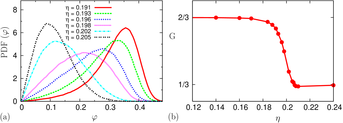
Figure 1: (a) The probability distribution function (PDF) of the order parameter $\varphi$ (defined in the text) for noise values $\eta$ around the critical point. The one humped curves indicate a second order phase transition. (b) The Binder cumulant $G$ (defined in the text) as a function of the noise. The smooth behavior of $G$ corroborates the second order nature of the disorder-order transition. The curves (a), (b) were obtained for the same parameters as in Ref. [12]: linear system size $L$ = 512, particle density $\rho$ = 1/8, velocity $v$ = 0.5 and we used $\simeq 300\tau$ MC simulation steps after observing the $\tau\simeq 10^{5}$ relaxation time.

3 The small velocity regime

The original model of Vicsek et al. was proposed to study the motion of bird flocks and/or bacterial colonies. The motion of the particles in such systems is quasi-continuous, i.e., usually the reaction time of the birds is significantly faster than the characteristic time that is needed to travel through their interaction radius ($R$). This condition imposes the following constraint on the update time $\Delta t$ in the numerical simulations: $\Delta t\ll R/v$, where $v$ is the magnitude of the particle velocity. After fixing the interaction radius $R$ = 1 and the update time $\Delta t$ = 1, the above condition becomes $v\ll$ 1. We refer to this velocity domain as the small velocity regime. Our further investigations (discussed below) showed that the small velocity regime actually holds for velocities $v\leq$ 0.1. There may be (relatively) rare situations when the large velocity regime ($v\geq 0.3$) used by Grégoire and Chaté [12] is a reasonable approximation of the flocking process (e.g., ’turbulent’ escape motion of birds during the attack of a predator), however, the physical justification of such situations is beyond the scope of the present paper. In the large velocity regime Ref. [12] finds density waves in the ordered state, objects that were not present in the simulations of Ref. [6]. We discuss the behavior of these planar waves occurring in the large velocity regime in the next section.

Intrigued by the possibility of finding density waves, we re-investigated the small velocity regime of [6] at larger system sizes and significantly longer simulation times. We carried out a series of runs for different velocities from $v$ = 0.01 to $v$ = 0.1. Typical snapshots of the behavior are shown in Fig. 2. On can see isolated and uncorrelated, but coherently moving flocks in the system. The flocks have reached their steady sizes. The nature of the disorder-order phase transition was characterized by the probability distribution function (PDF) of the order parameter $\varphi$ (average particle velocity).

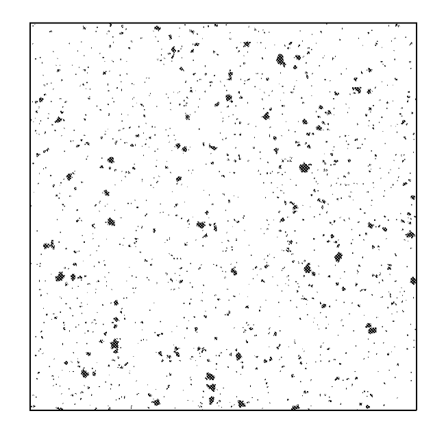
Figure 2: A typical snapshot of the system in the small velocity regime ($L$ = 512, $\rho$ = 1/8, and particle velocity $v$ = 0.1). One can observe isolated, but coherently moving flocks with a characteristic steady state size coexisting with a background gas of particles.

As shown in Fig. 3, the PDF was one humped, signaling a second order phase transition in accord with the earlier results of [6]. Furthermore, we also determined the corresponding Binder-cumulant $G$, defined above. We found that $G$ did not exhibit a significant minimum, corroborating the second order nature of the phase transition. On the other hand, the density waves, described by Ref. [12] in the large velocity regime, did not occur in the small velocity regime for tractable system sizes.

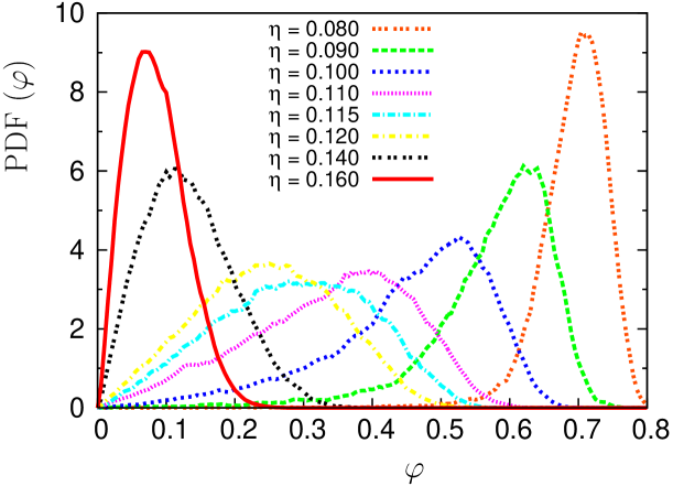
Figure 3: The PDF of the order parameter $\varphi$ in the small velocity regime ($v$ = 0.1) for noise values around the critical point. The one humped character of the curves demonstrates a second order phase transition. The curves were obtained for systems with linear system size $L$ = 512, particle density $\rho$ = 1/8 and we used $\simeq 100\tau$ MC simulation steps after observing the $\tau\simeq 10^{5}$ relaxation time.

4 The large velocity regime: boundary condition induced symmetry breaking and density waves

Our numerical studies showed that the density waves appear only in the ordered phase of the large velocity regime ($v\geq$ 0.3). In order to elucidate the emergence and nature of the density waves, we first determined the directional distribution of the average velocity in the ordered phase when density waves are present and found a strong anisotropy as shown in Fig. 4. It means that the density waves travel mainly parallel to sides of the simulation box or in other cases they travel in a diagonal direction. This, in fact implies that the periodic boundary conditions have a strong influence on the origin and behavior of the density waves.

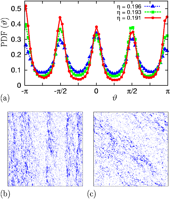
Figure 4: (a) The directional distribution of the average velocity in the large velocity regime ($v$ = 0.5) for the ordered state at three different values of noise. There is a strong anisotropy, i.e., particles preferentially move parallel to the sides of the simulation box (b) ($v$ = 3), or in other cases they move diagonally (c) ($v$ = 1). ($L$ = 512, $\rho$ = 1/8.)

To clarify this issue further we implemented a hexagonal simulation cell with hexagonal boundary conditions that display a threefold symmetry. We found that the directional distribution of the density waves followed the underlying symmetry of the boundary conditions as demonstrated in Fig. 5. Needless to say that such strong influences of the boundary conditions obscure the physical features and behavior in the large velocity regime of the SNM. Thus, it is impossible to gain a physical insight or to draw any conclusions in this regime.

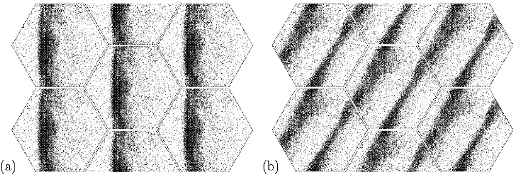
Figure 5: Snapshots of the spatial distribution of particles in the SNM for a hexagonal simulation cell. The central cell is repeated to demonstrate the implemented periodic boundary conditions (PBC). (a) A density wave traveling in one of the principal directions of the threefold hexagonal symmetry. (b) A density wave traveling in another principal direction of the hexagonal system. We found that the density waves move in directions determined by the underlying symmetry of the simulation cell in the large velocity regime ($v\geq$ 0.3). This directional quantization is a numerical artifact introduced by the presence of the PBC. ($L$ = 128/$\sqrt{3}$, $\rho$ = 2/$\sqrt{3}$, $v$ = 10.)

In spite of the above discussed principal limits of the physical interpretation in the large velocity regime, we also investigated this regime numerically. Our simulations indicated that at large particle velocities (e.g., $v$ = 10) the disorder-order transition exhibits a discontinuous order parameter and also a negative minimum in the Binder cumulant appears that are characteristic features of a first order phase transition (Fig. 6). Even though, in the light of the above it is not possible to justify this result on a physical basis, we note that a similar, lattice version of self-propelled particle models (Ref. [8]) also exhibits a first order phase transition. We suspect that the discontinuous phase transition behavior in both cases can be attributed to the broken and lowered symmetry in the system.

Furthermore, our numerical simulations showed that the phase transition became of second order again at extreme particle velocities ($v$ = 1000) in accord with a continuous mean-field like behavior. Thus, we witness that the nature of the disorder-order phase transition changes twice as a function of the particle velocity. The second order phase transition in the small velocity regime ($v\leq$ 0.1) is replaced by a first order transition like behavior (due to the periodic boundary condition induced unphysical symmetry breaking) for large particle velocities ($v\geq$ 0.3) and the phase transition is again of second order at extreme particle velocities. We emphasize though, that the apparent behavior can physically be justified only in the small velocity regime ($v\leq$ 0.1).

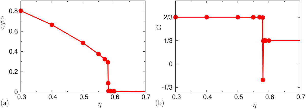
Figure 6: (a) The order parameter $\varphi$ as a function of the noise for a very large particle velocity ($v$ = 10). The discontinuous behavior of the order parameter indicates a first order phase transition. (b) The corresponding Binder cumulant $G$ displays a sharp and negative minimum at the phase transition point, characteristic to a first order transition. ($L$ = 256, $\rho$ = 1, and simulation time $10^{7}$ MC steps.)

5 Particle diffusion

In order to further investigate the SNM we studied diffusivity of the particles. To that purpose we took initially neighboring particles and determined their relative displacement parallel and perpendicular to the average velocity. To avoid the influence of the periodic boundary conditions, we considered only relative distances smaller than 1/10 of the linear system size $L$. Typical averaged square displacement curves as a function of the time can be seen in Fig. 7. We find a superdiffusive behavior at intermediate diffusion times in the ordered state: $<r^{2}>(t)\sim t^{\alpha}$ with $\alpha>$ 1. Furthermore, the diffusion is isotropic for small velocities and it becomes anisotropic at large particle velocities.

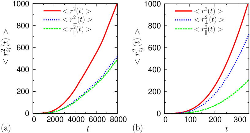
Figure 7: Averaged relative square displacements of initially neighboring particles as a function of time in the ordered phase ($\eta$ = 0.1). (a) The diffusion is isotropic in the small velocity regime ($v$ = 0.05), i.e., the relative square displacements are equal in the perpendicular and parallel directions relative to the average velocity. (b) At large particle velocities ($v$ = 0.5) the diffusion is anisotropic, i.e., the relative square displacement in the perpendicular direction ($<r^{2}_{\bot}>$) is significantly larger than that of in the parallel direction ($<r^{2}_{\|}>$). The curves also demonstrate the superdiffusive behavior at intermediate diffusion times: $<r^{2}>(t)\sim t^{\alpha}$ with $\alpha>$ 1. ($L$ = 256, $\rho$ = 1/8 and simulation time $10^{6}$ MC steps.)

The ratio of the square displacement components $A=r^{2}_{\bot}/r^{2}_{\|}$ measures the anisotropy of diffusion. Fig. 8 shows the anisotropy $A$ as a function of the velocity magnitude. At the velocity magnitude $v$ = 0.3 one can see a remarkable crossover from the isotropic diffusion to a strongly anisotropic one. Thus, while the diffusion is isotropic in the small velocity regime, it becomes highly anisotropic for larger velocities. We believe that the interplay between the anisotropic diffusion for larger velocities and the presence of the periodic boundary condition might be responsible for the emergence of the density waves in the large velocity regime.

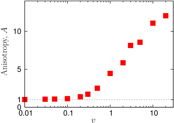
Figure 8: Anisotropy of the particle pair diffusion as a function of the particle velocity $v$: $A=r^{2}_{\bot}/r^{2}_{\|}$. One can clearly distinguish the small velocity regime ($v\leq$ 0.1) in which the diffusion is isotropic from the large velocity regime ($v\geq$ 0.3) with a strongly anisotropic diffusion. ($L$ = 256, $\rho$ = 1/8 and simulation time $10^{6}$ MC steps.)

We also measured the diffusion of initially neighboring particles as a function of noise strength. The relative mean square displacements of particles are presented in Fig. 9. At low noise levels one can distinguish three diffusion regimes. At small diffusion times, the diffusion process is almost frozen, particles keep their position relative to each other ($\alpha$ = 0). At intermediate times we witness superdiffusion ($\alpha>$ 1). Finally, at larger diffusion times, normal diffusion is recovered ($\alpha$ = 1). In order to characterize the extent of superdiffusion we measured the maximal diffusion exponent $\alpha_{max}$ by determining the maximal slope of the averaged logarithmic square displacement curves (Fig. 9). The noise dependence of the maximal diffusion exponent is plotted in Fig. 10. One can see that $\alpha_{max}$ decreases with increasing noise strength and reaches unity at about the noise strength $\eta$ = 0.5. We believe that this behavior is the consequence of the decay of flocks with increasing noise. Superdiffusion as well as crossover to normal diffusion were also observed and described in Refs. [12, 15] for similar models of collective motion.

Figure 9: The averaged relative square displacements of initially neighboring particles $<r^{2}_{ij}>$ as a function of time for different noise levels. Three types of behavior can be observed for low noise levels ($\eta<$ 0.5): At small diffusion times no relative diffusion occurs, at intermediate times superdiffusion dominates and at larger times normal diffusion is recovered. For high noise levels there is no superdiffusion due to the lack of coherently moving particle flocks. Three reference lines with slopes 1, 2, and 3 are also plotted in the figure for visual guidance. ($L$ = 512, $\rho$ = 1/8, $v=$ 0.1.)

Figure 10: The noise dependence of the maximal diffusion exponent $\alpha_{max}$. This curve was obtained by determining the maximal slope of the averaged logarithmic square displacement curves (Fig. 9). One can see in accord with Fig. 9 that there is no superdiffusion above a critical noise value ($\eta_{c}\simeq$ 0.5).

We interpret the above behavior for small noise strengths as follows. At short diffusion times, the majority of initially neighboring particles stay together in coherently moving and locally ordered flocks (see e.g., Fig. 2), thus, neighboring particles keep their positions relative to each other ($\alpha$ = 0). At intermediate times, i.e., times long enough for particles to change flocks for a few times, initially neighboring particles are carried away from each other in an ordered manner by the different flocks they belong to. It means that the mean spatial separation of the particle pairs increase roughly linearly with time and leads to a superdiffusion exponent ($\alpha\geq$ 2). At large diffusion times, flocks themselves perform random walks resulting in a normal diffusion of particle pairs ($\alpha$ = 1).

Finally, we studied the velocity dependence of the maximal diffusion exponent $\alpha_{max}$. Our results show that $\alpha_{max}$ varied between 1.5 and 3 in the superdiffusion time regime (Fig. 11).

Figure 11: The velocity dependence of the maximal diffusion exponent $\alpha_{max}$ at a low noise level ($\eta$ = 0.1). This curve shows that superdiffusion is always present below a critical noise value and crossover time. ($L$ = 256, $\rho$ = 1/8)

Conclusions

In this paper we presented our detailed investigations on the scalar noise model of collective motion. We justified the physical relevance of the small velocity regime ($v\leq$ 0.1) and performed extensive numerical simulations to re-investigate the order of the order-disorder phase transition in that regime. Our results corroborated the findings of Refs. [6, 7], i.e., the second order nature of the phase transition.

Furthermore, our numerical study of the large velocity regime ($v\geq$ 0.3) demonstrated the strong effects of the boundary conditions on the solutions. We found that the interplay between the anisotropic diffusion and the periodic boundary conditions introduced a numerical artifact, the directional quantization of the density waves. Thus, the presence of the boundary conditions makes it impossible to draw any conclusion about the physical behavior in the large velocity regime of the scalar noise model.

Finally, our detailed investigations indicate that the diffusion behavior of initially neighboring particles separates the small and the large velocity regimes. We find that the diffusion is isotropic for small particle velocities ($v\leq 0.1$), it becomes strongly anisotropic at large particle velocities ($v\geq 0.3$). Further investigations on the particle pair diffusion revealed particle superdiffusion with a crossover to the normal diffusion regime. The observed diverse behaviors demonstrate the richness of physics exhibited by this simple model.

This work has been supported by the Hungarian Science Foundation (OTKA), grant No. T049674 and EU FP6 Grant ”Starflag”.

References

- [1] S. H. Strogatz and I. Stewart, Scientific American 269, 102 (1993).
- [2] C. J. Feare, The starlings, Oxford University Press, 1984; J. K. Parrish and W. H. Hamner, eds., Animal groups in three dimensions, Cambridge University Press, 1997 (and references therein); C. W. Reynolds, Comp. Graph. 21, 25 (1987).
- [3] J. K. Parrish and L. Edelstein-Keshet, Science 284, 99 (1999); T. Inagaki, W. Sakamoto and T. Kuroki, Bull. Jap. Soc. Sci. Fish, 42, 265 (1976).
- [4] E. M. Rauch, M. M. Millonas and D. R. Chialvo, Phys. Lett. A, 207, 185 (1995).
- [5] E. Ben-Jacob, I. Cohen, O. Shochet, A. Czirók and T. Vicsek, Phys. Rev. Lett. 75, 2899 (1995); J. A. Shapiro, BioEssays 17, 597 (1995); J. A. Shapiro and M. Dworkin, eds., Bacteria as multicellular organisms, Oxford University Press, 1997.
- [6] T. Vicsek, A. Czirók, E. Ben-Jacob, I. Cohen and O. Shochet Phys. Rev. Lett. 75, 1226 (1995).
- [7] A. Czirók, H. E. Stanley and T. Vicsek, J. Phys A 30, 1375 (1997).
- [8] Z. Csahók and T. Vicsek, Phys. Rev. E 52, 5297 (1995).
- [9] J. Toner and Y. Tu, Phys. Rev. Lett. 75, 4326 (1995).
- [10] J. Toner, Y. Tu and M. Ulm, Phys. Rev. Lett. 80, 4819 (1998).
- [11] J. Toner and Y. Tu, Phys. Rev. E 58, 4828 (1998).
- [12] G. Grégoire and H. Chaté, Phys. Rev. Lett. 92, 025702 (2004).
- [13] C. Huepe and M. Aldana, Phys. Rev. Lett. 92, 168701 (2004).
- [14] K. Binder and D. W. Herrmann, Monte Carlo Simulation in Statistical Physics, Springer (1997).
- [15] G. Grégoire, H. Chaté and Y. Tu, Phys. Rev. E 64, 011902 (2001); G. Grégoire, H. Chaté and Y. Tu, Physica D 181, 157 (2003).