One-dimensional solitary waves in singular deformations of $SO(2)$ invariant two-component scalar field theory models

Abstract

In this paper we study the structure of the manifold of solitary waves in some deformations of $SO(2)$ symmetric two-component scalar field theoretical models in two-dimensional Minkowski space. The deformation is chosen in order to make the analogous mechanical system Hamilton-Jacobi separable in polar coordinates and displays a singularity at the origin of the internal plane. The existence of the singularity confers interesting and intriguing properties to the solitary waves or kink solutions.

1 Introduction

Solitary waves are at the heart of astonishing phenomena in diverse physical systems that can be modeled by non-linear equations. For instance, they describe the behavior of interfaces in magnetic materials [2] and in ferroelectric crystals [3] in Condensed Matter. Solitary waves have biotechnical and biomedical applications [4] and also seed the formation of structures in Cosmology [5]. In several disguises, kinks, topological defects, domain walls, membranes, solitary waves arise in many branches of Theoretical Physics [6, 7]. For this reason, the search for solitary waves in some types of PDE is an active topic in non-linear science. Among these equations we find the non-linear Klein-Gordon equation, extensively cited in the physical literature [8, 9]. This equation, generalized to $N$-real scalar fields, reads as follows:

$$\frac{\partial^{2}\phi_{a}}{\partial t^{2}}-\frac{\partial^{2}\phi_{a}}{\partial x^{2}}+\frac{\partial U}{\partial\phi_{a}}=0\hskip 28.45274pta=1,2,\dots,N\qquad,$$ (1)

where $U(\phi_{1},\dots,\phi_{N})$ is a potential function of the scalar fields $\phi_{a}$, whereas $\frac{\partial U}{\partial\phi_{a}}$ are non-linear functions of the fields. PDE (1) can be understood as the Euler-Lagrange equations associated with the functional action

$$S=\int d^{2}x\left[\frac{1}{2}\sum_{a=1}^{N}\partial_{\mu}\phi^{a}\partial^{\mu}\phi^{a}-U(\phi_{1},...,\phi_{N})\right]$$

governing the dynamics of a (1+1) dimensional scalar field theory. In this framework, a solitary wave is a localized non-singular solution of the non-linear field equation (1) whose energy density, as well as being localized, has space-time dependence of the form: $\varepsilon(t,x)=\varepsilon(x-\mbox{v}t)$, where v is some velocity vector according to Rajaraman [9]. Use of Lorentz invariance allows us to investigate the existence of some kinds of solitary waves by reducing PDE (1) to the following ODE:

$$\frac{\partial^{2}\phi_{a}}{\partial x^{2}}=\frac{\partial U}{\partial\phi_{a}}\hskip 28.45274pta=1,2,\dots,N\qquad.$$ (2)

Therefore, the search for solitary waves or kinks, finite energy solutions to the static field equations (2), is tantamount to solving a analogous mechanical problem for a unit-mass point particle moving in a plane with coordinates $\phi=(\phi_{1},\phi_{2})$ under the influence of a potential $-U(\phi)$, if the variable $x$ plays the r$\hat{\rm o}$le of “time” [9].

The sine-Gordon and $\phi^{4}$ models, profusely dealt with in the literature, are the basic examples of (1), respectively governed by the PDE equations:

$$\frac{\partial^{2}\phi}{\partial t^{2}}-\frac{\partial^{2}\phi}{\partial x^{2}}+\sin\phi=0\hskip 56.9055pt\frac{\partial^{2}\phi}{\partial t^{2}}-\frac{\partial^{2}\phi}{\partial x^{2}}+2\phi(1-\phi^{2})=0\qquad.$$

The corresponding potential terms are $U(\phi)=1-\cos\phi$ and $U(\phi)=\frac{1}{2}(\phi^{2}-1)^{2}$ and for both systems solitary or traveling wave solutions exist: the well known sine-Gordon soliton and $\lambda(\phi)^{4}_{2}$ kink. The peculiar non-dispersive character of these non-linear waves is related to the structure of the set ${\cal M}$ of zeroes of the potential $U(\phi)$. ${\cal M}$ is a discrete set with more than one element. The field profile of these solitary waves connects two elements of ${\cal M}$ asymptotically. For instance, the kink $\phi_{K}(x)=\mp{\rm tanh}x$ in the $\phi^{4}$ model interpolates between the two zeroes $\phi_{\pm}=\pm 1$ of $U(\phi)$: $\phi_{K}(x=-\infty)=\pm 1$, $\phi_{K}(x=\infty)=\mp 1$. Obviously, the greater the number of elements in ${\cal M}$, the richer the solitary wave variety. Thus, other models have been considered in the literature in the search for these kinds of non-linear waves, such as the $\phi^{6}$ model with potential $U(\phi)=\frac{1}{2}\phi^{2}(\phi^{2}-1)^{2}$, the $\phi^{8}$ model with $U(\phi)=\frac{1}{2}(\phi^{2}-1)^{2}(\phi^{2}-a^{2})^{2}$ in the one-component scalar field theory framework [10] and, more recently, polynomial interactions of any order built from Chebyshev polynomials [11].

Another way of obtaining a richer structure in the set ${\cal M}$, and hence in the solitary wave manifold, is to increase the dimension of the internal space, i.e, by considering theories with more scalar field components. This is an important qualitative step, as noted by Rajaraman [9]: This already brings us to the stage where no general methods are available for obtaining all localized static solutions, given the field equations. However, some solutions, but by no means all, can be obtained for a class of such Lagrangians using a little trial and error.

Straightforward generalization of the $\phi^{4}$ and $\phi^{8}$ models to two-component scalar field theory leads to the potential energy densities:

$$v^{(A)}(\phi_{1},\phi_{2}) = (\phi_{1}^{2}+\phi_{2}^{2}-1)^{2}$$ (3)

$$v^{(B)}(\phi_{1},\phi_{2}) = (\phi_{1}^{2}+\phi_{2}^{2}-1)^{2}(\phi_{1}^{2}+\phi_{2}^{2}-a^{2})^{2}\qquad.$$ (4)

The action functional is invariant under $SO(2)$ rotations in the $\phi_{1}-\phi_{2}$ internal plane. The zeroes of $v^{(A)}$ and $v^{(B)}$, however, are not invariant under the $SO(2)$ action and the orbits, ${\cal M}$, are continuous manifolds in these cases: ${\cal M}^{(A)}=S_{1}^{R=1}$, ${\cal M}^{(B)}=S_{1}^{R=1}\cup S_{1}^{R=a}$, respectively. Goldstone bosons arise in the process of quantification in this situation. Coleman proved in [12] that there are no Goldstone bosons in a sensible scalar field theory on the line. The infrared asymptotic behavior of quantum theory would require the modification of the potentials $v^{(A)}$ and $v^{(B)}$ in such a way that their manifold of zeroes becomes a discrete set. Thus, the effect of quantum fluctuations is to add perturbations to the potentials (3) and (4)

$$U(\phi_{1},\phi_{2})=v^{(A,B)}(\phi_{1},\phi_{2})+w(\phi_{1},\phi_{2})$$

such that the $SO(2)$ symmetry is explicitly broken down into discrete subgroups -acting on the new discrete sets of zeroes- whereas the $U(\phi_{1},\phi_{2})$ potential energy density remains a non-negative expression.

There are some models in the literature that match these features. The best studied is the MSTB model, with potential energy density:

$$U_{\rm MSTB}(\phi_{1},\phi_{2})=v^{(A)}(\phi_{1},\phi_{2})+\sigma^{2}\phi_{2}^{2}\qquad,$$

where $\sigma$ is a non-dimensional parameter. It was first proposed by Montonen [13] and Sarker, Trullinger and Bishop [14]. Rajaraman and Weinberg [15] discovered two kinds of kinks by the trial orbit method; the TK1 (one-topological kinks) - tracing a straight line trajectory in the analogous mechanical system- and the TK2 (two-component topological kinks) - running through semi-elliptic orbits in the mechanical system. These enquiries were followed by numerical analysis [16, 17] and with this method Subbaswamy and Trullinger found the existence of a whole family of two-component non-topological kinks, which were named as NTK. Moreover, they discovered an unexpected fact: the NTK energy is equal to the addition of the TK1 and TK2 energies. This relation is known as the kink mass “sum rule”. In 1985, Ito explained all of these issues analytically. The crux of the matter is the separability of the Hamilton-Jacobi equation using elliptic coordinates in the analogous mechanical system [18, 19, 20, 21]. Unlike models with only one scalar field, systems with two or more scalar fields have analogous mechanical systems that are generically non-integrable. The analogous mechanical system of the MSTB model is a completely integrable Type I Liouville model - separable in elliptic coordinates- and all the solitary waves can be found analytically . Other models exhibiting similar properties have been addressed in References [22, 23, 24]. The generalization of this kind of model to three-component scalar field theory is studied in [25, 26, 27].

The goal of this work is to identify the variety of solitary wave or kink solutions in a broad family of models arising from perturbations of the $SO(2)$ symmetric two-component scalar field $\phi^{4}$ and $\phi^{8}$ models (3) and (4). The strategy will be to deal with analogous mechanical systems of Liouville Type II, i. e., with Hamilton-Jacobi equations separable in polar coordinates. These deformations necessarily involve a singularity at the origin of the configuration space in the mechanical system, equivalently, at the origin of the internal plane in the field theoretical model. Strictly speaking, the perturbation does not exist as a proper function when $\phi_{1}=\phi_{2}=0$ because the limit of $w(\phi_{1},\phi_{2})$ when both $\phi_{1}$ and $\phi_{2}$ are zero is either $0$ or $\infty$, depending on the path followed to reach $w(0,0)$. This mathematical pathology confers new and intriguing properties to solitary wave solutions. For example, certain kink profiles connecting identical vacuum points in internal space asymptotically cannot be deformed into each other even though they belong to the same topological sector in the configuration space. Trajectories moving away from the origin involve infinite energy and some kink solutions behave as strings pinned at one point in internal space. Nevertheless, we shall show that in the four models that we discussed here there is a plethora of kink or solitary wave solutions, including topological and non-topological kinks, one-parametric kink families, and singular solutions.

The organization of the paper is as follows: In Section §2 we shall describe the models to be studied from a generic point of view. We shall discuss the general properties of these models and state three interesting results. In Sections §3, §4, §5 and §6 we shall deal with the particular models that correspond to two perturbations of (3) and (4). Applying the procedure explained in Section §2, we shall describe in detail the solitary wave solutions arising in these systems and unveil their hidden structure.

2 Generalities

In the models that we shall study, the (non-dimensional) scalar fields,

$$\vec{\phi}(x_{0},x_{1})=(\phi_{1}(x_{0},x_{1}),\phi_{2}(x_{0},x_{1})):\mathbb{R}^{1,1}\rightarrow\mathbb{R}^{2}$$

are maps from (1+1)-dimensional Minkowskian space-time ${\mathbb{R}}^{1,1}$ to the ${\mathbb{R}}^{2}$ internal space. The action functional

$$S=\int d^{2}x\left[\frac{1}{2}\sum_{a=1}^{2}\partial_{\mu}\phi^{a}\partial^{\nu}\phi^{a}-U(\phi_{1},\phi_{2})\right]$$ (5)

is invariant under the Poincaré transformations acting on ${\mathbb{R}}^{1,1}$, whereas the remaining symmetry transformations of our models belong to the subgroup of $SO(2)$ rotations in the internal plane ${\mathbb{R}}^{2}$ that do not change $U(\phi_{1},\phi_{2})$. Our convention for the metric tensor components in Minkowski space ${\mathbb{R}}^{1,1}$ is $g_{00}=-g_{11}=1$, $g_{12}=g_{21}=0$ and only non-dimensional parameters will be considered throughout the paper.

A “point” in the configuration space of the system is a configuration of the field of finite energy; i.e., a picture of the field at a fixed time such that the energy $E$, the integral over the real line of the energy density,

$$E[\vec{\phi}]=\int_{-\infty}^{\infty}dx{\cal E}[\vec{\phi}]\qquad,\qquad{\cal E}[\vec{\phi}]=\frac{1}{2}\left(\frac{d\phi_{1}}{dx}\right)^{2}+\frac{1}{2}\left(\frac{d\phi_{2}}{dx}\right)^{2}+U(\phi_{1},\phi_{2})$$ (6)

is finite. Thus, the configuration space is the set of continuous maps from ${\mathbb{R}}$ to ${\mathbb{R}}^{2}$ of finite energy:

$${\cal C}=\left\{\vec{\phi}(x)\in{\rm Maps}({\mathbb{R}},{\mathbb{R}}^{2})/E<\infty\right\}\qquad.$$

In order to belong to ${\cal C}$, each configuration must comply with the asymptotic conditions

$$\lim_{x\rightarrow\pm\infty}\vec{\phi}\in{\cal M}\hskip 56.9055pt\lim_{x\rightarrow\pm\infty}\frac{d\vec{\phi}}{dx}=0\qquad,$$ (7)

where ${\cal M}$ is the set of zeroes (minima) of the potential term $U(\vec{\phi})$.

We shall analyze four different models, deforming the $\phi^{4}$ and $\phi^{8}$ potential energy densities (3) and (4) by two classes of perturbations:

$$w^{(1)}(\phi_{1},\phi_{2}) = \frac{\sigma^{2}\phi_{2}^{2}}{(\phi_{1}^{2}+\phi_{2}^{2})^{2}}$$ (8)

$$w^{(2)}(\phi_{1},\phi_{2}) = \frac{\sigma^{2}}{2(\phi_{1}^{2}+\phi_{2}^{2})}\left(1-\frac{\phi_{1}}{\sqrt{\phi_{1}^{2}+\phi_{2}^{2}}}\right)\qquad,$$ (9)

where $\sigma$ is a non-dimensional coupling constant of the system. Thus, we consider four distinct potential energy densities $U(\phi_{1},\phi_{2})$ labelled as follows:

$$U^{(IJ)}(\phi_{1},\phi_{2})=v^{(I)}(\phi_{1},\phi_{2})+w^{(J)}(\phi_{1},\phi_{2})\qquad,$$ (10)

where $I=A,B$ and $J=1,2$.

An important remark should be made here: both $w^{(1)}$ and $w^{(2)}$ are singular at the origin. The limit of $w^{(2)}(\phi_{1},\phi_{2})$ when $\phi_{1}\rightarrow 0$, $\phi_{2}\rightarrow 0$ is always infinite, independently of the path chosen in ${\mathbb{R}}^{2}$ to approach the origin. $\lim_{(\phi_{1},\phi_{2})\rightarrow(0,0)}w^{(1)}(\phi_{1},\phi_{2})$ is, however, finite, zero, if the origin is approached through the abscissa axis $\phi_{2}=0$, but it is equal to infinity for any other approaching path. Therefore, field profiles passing through the origin have infinite energy and are excluded from the configuration space in all of four cases, except field configurations such that all their derivatives along the $\phi_{2}$ axis at the origin vanish when the perturbation chosen is $w^{(1)}$.

The invariance of the system of ODE (2) under spatial translations, $x\rightarrow x-x_{0}$ and reflections $x\rightarrow-x$ makes it convenient to abbreviate the notation: $\bar{x}=(-1)^{\delta}(x-x_{0})$, $x_{0}\in\mathbb{R}$, $\delta=0,1$. In this manner, we shall describe a whole family of kinks and anti-kinks with their centers located at arbitrary points on the line, because these symmetry transformations bring solutions into solutions.

The use of polar coordinates in the internal space ${\mathbb{R}}^{2}$ is suggested by the $SO(2)$ invariance of $v^{(A)}$ and $v^{(B)}$ as well as by the choice of perturbations $w^{(1)}$ and $w^{(2)}$. This system of coordinates is defined by the diffeomorphism

$$\begin{array}[]{cccc}\zeta:&\mathbb{R}^{+}\times S^{1}&\longrightarrow&\mathbb{R}^{2}\\ &(R_{0},\varphi_{0})&\longrightarrow&(\phi_{1}^{0},\phi_{2}^{0})\end{array}\hskip 28.45274pt\left\{\begin{array}[]{l}\zeta^{*}(\phi_{1})=R\cos\varphi\\ \zeta^{*}(\phi_{2})=R\sin\varphi\end{array}\right.$$

$$\quad 0\leq R=+\sqrt{\phi_{1}^{2}+\phi_{2}^{2}}\leq\infty\qquad\qquad,\qquad\qquad 0\leq\varphi={\rm arctan}{\phi_{2}\over\phi_{1}}<2\pi\qquad.$$

By using polar coordinates, $v^{(A)}$, $v^{(B)}$, $w^{(1)}$ and $v^{(2)}$ become:

$$f^{(A)}(R)=\zeta^{*}v^{(A)}=(R^{2}-1)^{2}\hskip 28.45274pt;\hskip 34.14322ptf^{(B)}(R)=\zeta^{*}v^{(B)}=(R^{2}-1)^{2}(R^{2}-a)^{2}\hskip 5.69046pt;$$

$${1\over R^{2}}g^{(1)}(\varphi)=\zeta^{*}w^{(1)}=\frac{\sigma^{2}}{R^{2}}\sin^{2}\varphi\hskip 34.14322pt;\hskip 34.14322pt{1\over R^{2}}g^{(2)}(\varphi)=\zeta^{*}w^{(2)}=\frac{\sigma^{2}}{R^{2}}\sin^{2}\frac{\varphi}{2}\qquad.$$

Thus, the first summand in (10) is a function $f^{(I)}(R)$ that depends only on the radial variable. The second summand in (10) is the product of a function $g^{(J)}(\varphi)$ depending only on the angular variable times the square of the inverse of $R$:

$$\zeta^{*}(U^{(IJ)})=f^{(I)}(R)+\frac{1}{R^{2}}g^{(J)}(\varphi)\qquad.$$ (12)

We shall refer to this class of systems as Type II Liouville models after the type of their analogous integrable mechanical systems [28]. We see the reason for the inevitability of the singularity at $R=0$: the factor ${1\over R^{2}}$ in the second summand of $U^{(IJ)}(R,\varphi)$. In $w^{(1)}$, however, the singularity is not seen if the origin is reached through the paths $\varphi=\pi$ and $\varphi=0$. In the other case, $w^{(2)}$, only passing through the origin via $\varphi=0$ kills the singularity, but there is no continuous way out and the “particle” would become entrapped by the singularity.

The general structure of the set ${\cal M}$ of zeroes of the potential energy density is easy to unveil: $\zeta^{*}(U)$ vanishes if and only if the two summands on the right hand side of formula (12) are zero. Thus,

$$\zeta^{*}{\cal M} = \{(R_{i},\varphi_{j})\in\mathbb{R}^{+}\times S^{1}\,/\,f^{(I)}(R_{i})=0\,\,,\,\,g^{(J)}(\varphi_{j})=0\,\,,\,\,\,i=1,...,M\,\,,\,\,\,j=1,...,N\}$$

and the $M\times N$ points $(R_{i},\varphi_{j})\in\zeta^{*}{\cal M}$ lie on the knots of a lattice where the laths are the two sets of perpendicular straight lines:

$$r_{R}=\{R=R_{i},i=1,...,M\}\hskip 28.45274pt\mbox{and}\hskip 28.45274ptr_{\varphi}=\{\varphi=\varphi_{j},j=1,...,N\}\qquad.$$

These lines are separatrix curves: there are no bounded trajectories crossing these boundaries. In the field theoretical context, static solutions are also enclosed in these domains.

Using polar coordinates, the energy functional reads:

$$\zeta^{*}E=\int\left[\frac{1}{2}\left(\frac{dR}{dx}\right)^{2}+\frac{1}{2}R^{2}\left(\frac{d\varphi}{dx}\right)^{2}+f(R)+\frac{1}{R^{2}}g(\varphi)\right]\qquad.$$ (13)

One can think of this functional in (13) either as the static energy of the scalar field or, alternatively, as the action functional for a particle of unit mass and $(R,\varphi)$ position coordinates moving under the influence of a potential $-\zeta^{*}{U}(R,\varphi)=-\left(f(R)+\frac{1}{R^{2}}g(\varphi)\right)$ with evolution parameter $x$. Thus, the motion equations of this analogous mechanical system are the ODE system:

$$\frac{d^{2}R}{dx^{2}}=\frac{df(R)}{dR}\hskip 28.45274pt;\hskip 28.45274ptR^{2}\frac{d^{2}\varphi}{dx^{2}}+\frac{dR}{dx}\frac{d\varphi}{dx}=\frac{dg(\varphi)}{d\varphi}\qquad.$$ (14)

Lorentz invariance guarantees that finite action solutions of (14) are traveling waves of the scalar field theory with their center of mass located at the origin; Lorentz and translation transformations provide all the solitary wave solutions of the system obtained from the static ones by applying the appropriate transformations.

To solve the ODE (14), we take advantage of the existence of two independent first-integrals in the mechanical system, namely:

$$I_{1}=\frac{1}{2}\left(\frac{dR}{dx}\right)^{2}+\frac{1}{2}R^{2}\left(\frac{d\varphi}{dx}\right)^{2}-f(R)-\frac{1}{R^{2}}g(\varphi)\hskip 22.76228pt;\hskip 22.76228ptI_{2}=\frac{1}{2}R^{4}\left(\frac{d\varphi}{dx}\right)^{2}-g(\varphi)\qquad.$$ (15)

$I_{1}$ and $I_{2}$ are respectively the energy and the generalized angular momentum in the analogous mechanical system. Written in polar coordinates, the asymptotic conditions (7) guaranteeing finite energy in the field theory model read:

$$\lim_{x\rightarrow\pm\infty}(R(x),\varphi(x))=(R_{i_{\pm}},\varphi_{j_{\pm}})\in\zeta^{*}{\cal M}\quad,\quad\lim_{x\rightarrow\pm\infty}{dR\over dx}(x)=0\quad,\quad\lim_{x\rightarrow\pm\infty}{d\varphi\over dx}(x)=0\qquad.$$ (16)

Thus, $I_{1}(x=\pm\infty)=0$ and $I_{2}(x=\pm\infty)=0$; because $I_{1}$ and $I_{2}$ are invariants of the mechanical system they vanish for every point $x\in\mathbb{R}$. Therefore, solitary wave solutions of scalar field theory are in one-to-one correspondence (modulo Lorentz boosts) with the trajectories of the mechanical analogous system such that $I_{1}=0$, $I_{2}=0$, i.e., trajectories solving the following first-order ODE system:

$$\frac{dR}{dx}=(-1)^{\alpha}\sqrt{2f(R)}\qquad\qquad,\qquad\qquad\frac{d\varphi}{dx}=(-1)^{\beta}{1\over R^{2}}\sqrt{2g(\varphi)}\quad,\quad\alpha,\beta=0,1\quad.$$ (17)

We now state the first result concerning the structure of the solitary wave variety in Type II Liouville models:

Proposition 1.- There exist kink or solitary wave solutions whose orbits lie on the separatrix straight lines. Kink orbits are of two kinds: 1) those connecting two elements $(R_{i},\varphi_{j})$ and $(R_{i+1},\varphi_{j})$ of ${\cal M}$ through a straight segment $(R(x),\varphi_{j})$ (angular rays in the Cartesian internal plane) and 2) those joining the vacuum points $(R_{i},\varphi_{j})$ and $(R_{i},\varphi_{j+1})$ through the straight line $(R_{i},\varphi(x))$ (circles on the Cartesian internal plane).

The proof is easy: note that the vanishing of the first integrals $I_{1}=0,I_{2}=0$ along the kink orbits and the assumption of the existence of solutions whose orbit is $R=R_{i}$ or $\varphi=\varphi_{j}$ on the polar internal plane, $R_{i}$ and $\varphi_{j}$ being respectively roots of the functions $f(R)$ and $g(\varphi)$, are compatible conditions. We distinguish two possible cases:

• If $R=R_{i}$,

  $$I_{1}=\frac{1}{2}R_{i}^{2}\left(\frac{d\varphi}{dx}\right)^{2}-\frac{1}{R_{i}^{2}}g(\varphi)=0=\frac{1}{R_{i}^{2}}I_{2}$$

  holds and the problem of finding the time-schedule or kink form factor is solved by the quadrature:

  $$G[\varphi]=\int\,\frac{d\varphi}{\sqrt{2g(\varphi)}}\qquad,\qquad\varphi^{K}(x)=G^{-1}\left(\frac{\bar{x}}{R_{i}^{2}}\right)\qquad.$$

• If $\varphi=\varphi_{j}$, the two invariants become

  $$I_{1}=\frac{1}{2}\left(\frac{dR}{dx}\right)^{2}-f(R)=0\hskip 28.45274pt,\hskip 28.45274ptI_{2}=\frac{1}{2}g(\varphi_{j})=0\qquad.$$

  The vanishing of $I_{2}$ turns into a identity but the first-order equation annihilating $I_{1}$ provides the kink form factor by means of the quadrature:

  $$F[R]=\int\,\frac{dR}{\sqrt{2f(R)}}\qquad,\qquad R^{K}(x)=F^{-1}(\bar{x})\qquad.$$

To obtain all the separatrix orbits -those for which $I_{1}=0$ and $I_{2}=0$, in Type II Liouville models- it is convenient to apply the Hamilton-Jacobi procedure because the HJ equation is separable in polar coordinates and all the trajectories can be found by quadratures. The generalized momenta are $p_{R}=\frac{dR}{dx}$ and $p_{\varphi}=R^{2}\frac{d\varphi}{dx}$, whereas the mechanical Hamiltonian (or Hamiltonian energy density in the field theory) is:

$${\cal H}=h_{R}+\frac{1}{R^{2}}h_{\varphi}\hskip 28.45274pt,\hskip 28.45274pth_{R}=\frac{1}{2}p_{R}^{2}-f(R)\hskip 28.45274pt,\hskip 28.45274pth_{\varphi}=\frac{1}{2}p_{\varphi}^{2}-g(\varphi)\qquad.$$

The ansatz of separation of variables ${\cal J}={\cal J}_{R}(R)+{\cal J}_{\varphi}(\varphi)-i_{1}x$ for the Hamilton principal function ${\cal J}$ converts the PDE Hamilton-Jacobi equation

$$\frac{\partial{\cal J}}{\partial x}+{\cal H}\left(\frac{\partial{\cal J}}{\partial R},\frac{\partial{\cal J}}{\partial\varphi},R,\varphi\right)=0$$

into the ODE system:

$${1\over 2}\left(\frac{d{\cal J}_{R}}{dR}\right)^{2}-f(R)-{i_{2}\over R^{2}}=i_{1}\qquad,\qquad{1\over 2}\left(\frac{d{\cal J}_{\varphi}}{d\varphi}\right)^{2}-g(\varphi)=-i_{2}\quad;\quad i_{1},i_{2}\in\mathbb{R}\qquad.$$ (18)

Therefore, the Hamilton characteristic function is given by the quadratures

$${\cal J}_{R}(R)={\rm sign}(p_{R})\,\sqrt{2}\int dR\sqrt{f(R)+i_{1}+\frac{i_{2}}{R^{2}}}\qquad,\qquad{\cal J}_{\varphi}(\varphi)={\rm sign}(p_{\varphi})\,\sqrt{2}\int d\varphi\sqrt{g(\varphi)-i_{2}}\quad,$$

and the kink solutions comply with the equations:

• “Orbit” equation: $\left.\frac{\partial{\cal J}}{\partial i_{2}}\right|_{i_{1}=0=i_{2}}=\gamma_{1}$,

  $${\rm sign}(p_{R})\int\frac{dR}{R^{2}\sqrt{2f(R)}}-{\rm sign}(p_{\varphi})\int\frac{d\varphi}{\sqrt{2g(\varphi)}}=\gamma_{1}$$ (19)

• “Time schedule”: $\left.\frac{\partial{\cal J}}{\partial i_{1}}\right|_{i_{1}=0=i_{2}}=\gamma_{2}$,

  $${\rm sign}(p_{R})\int\frac{dR}{\sqrt{2f(R)}}=x+\gamma_{2}\qquad.$$ (20)

To unveil how the special orbits $R=R_{i}$ and $\varphi=\varphi_{j}$ are hidden in the family of trajectories parametrized by $\gamma_{1}$ and $\gamma_{2}$, it is useful to show explicitly the connection between the systems of equations (17) and (19)-(20). To fulfil this goal, we derive from (17) three identities:

$$\int\,\frac{dR}{\sqrt{2f(R)}} = \bar{x}$$ (21)

$$\int\,\frac{dR}{(-1)^{\alpha}R^{2}\sqrt{2f(R)}} = \int\,\frac{dx}{R^{2}(x)}+c$$ (22)

$$\int\,\frac{d\varphi}{(-1)^{\beta}\sqrt{2g(\varphi)}} = \int\,\frac{dx}{R^{2}(x)}+d$$ (23)

It is clear that (21) is equal to (20), whereas subtracting (23) from (22) one obtains (19) if $\gamma_{1}=c-d$ and ${\rm sign}(p_{\varphi})=(-1)^{\beta}$. The straight line orbits arise when $|\gamma_{1}|=\infty$. In this limit, the (19)-(20) system makes sense only if (a) $\varphi(x)=\varphi_{j}$ is the orbit, $g(\varphi_{j})=0$, and the time schedule (kink form factor or kink profile) is obtained by integrating (20); (b) $R(x)=R_{i}$ is the orbit, $f(R_{i})=0$, and the time schedule is obtained by integrating (23). Thus, the special straight line orbits are at the boundary of the family of kink trajectories.

Because the kink energy is the action of the associated separatrix trajectory in the analogous mechanical system –$\left|{\cal J}_{R}\right|+\left|{\cal J}_{\varphi}\right|$ computed along the kink path– we state:

Proposition 2.- The energy associated to a kink or solitary wave solution in the Type II Liouville models is:

$${\cal E}[\phi(x)]=\left|\int_{\pi_{r}(\zeta^{*}\phi)}dR\sqrt{2f(R)}\right|+\left|\int_{\pi_{\varphi}(\zeta^{*}\phi)}d\varphi\sqrt{2g(\varphi)}\right|\qquad.$$

Here, $\pi_{R}$ and $\pi_{\varphi}$ are the projectors onto the $R$- and $\varphi$-axes in the polar cylinder $\mathbb{R}^{+}\times\mathbb{S}^{1}$; application of these projectors to the $x$-parametrized kink paths allows us to trade the path integration along complicated curves by the sum of integrations along straight $R(x)=R_{i}$ and $\varphi(x)=\varphi_{j}$ lines. This is the rationale underlying the kink energy sum rules: all the kinks or combinations of kinks having the same projections to the polar axes carry the same energy.

To close this Section on generalities, we briefly describe how the analogous mechanical system is related to supersymmetry. In supersymmetric classical mechanics all the interactions are derived from a superpotential $W(\phi_{1},\phi_{2})$ [29, 30], related to the mechanical potential energy through the equation:

$$U(\phi_{1},\phi_{2})=\frac{1}{2}\left(\frac{\partial W}{\partial\phi_{1}}\right)^{2}+\frac{1}{2}\left(\frac{\partial W}{\partial\phi_{2}}\right)^{2}\qquad.$$ (24)

This is no more than the Hamilton-Jacobi equation for $i_{1}=0$ of a mechanical system with flipped potential energy $V(\phi_{1},\phi_{2})=-U(\phi_{1},\phi_{2})$ (precisely as in the analogous mechanical system), and the superpotential is tantamount to the Hamilton characteristic function. The mechanical action reads:

$$E={1\over 2}\int\,dx\,\left(\frac{d\phi_{1}}{dx}\frac{d\phi_{1}}{dx}+\frac{d\phi_{2}}{dx}\frac{d\phi_{2}}{dx}+\frac{\partial W}{\partial\phi_{1}}\frac{\partial W}{\partial\phi_{1}}+\frac{\partial W}{\partial\phi_{2}}\frac{\partial W}{\partial\phi_{2}}\right)$$

and this can be arranged ${\rm a}^{\prime}$ la Bogomolny [31]:

$$E={1\over 2}\int\,dx\,\left[\left(\frac{d\phi_{1}}{dx}-\frac{\partial W}{\partial\phi_{1}}\right)^{2}+\left(\frac{d\phi_{2}}{dx}-\frac{\partial W}{\partial\phi_{2}}\right)^{2}\right]+\int\,\left(d\phi_{1}\frac{\partial W}{\partial\phi_{1}}+d\phi_{2}\frac{\partial W}{\partial\phi_{1}}\right)\qquad.$$

Thus, the Bogomolny bound $E_{B}=\left|\int\,dW\right|$ is attained by solutions of the first-order differential equations:

$$\frac{d\phi_{1}}{dx}=\frac{\partial W}{\partial\phi_{1}}\hskip 56.9055pt,\hskip 56.9055pt\frac{d\phi_{2}}{dx}=\frac{\partial W}{\partial\phi_{2}}\qquad.$$ (25)

Because a first-order ODE system such as (25) is easier to solve than second-order motion equations, it is important to know when the PDE equation (24) is solvable. Hamilton-Jacobi separable systems admit a complete solution of such an equation and for Type II Liouville systems the situation is:

Proposition 3. Type II Liouville models admit four superpotentials.

Proof. In polar coordinates (24) reads:

$$\frac{1}{2}\left[\left(\frac{\partial W}{\partial R}\right)^{2}+\frac{1}{R^{2}}\left(\frac{\partial W}{\partial\varphi}\right)^{2}\right]=f(R)+\frac{1}{R^{2}}g(\varphi)\qquad.$$ (26)

Searching for solutions of (26) such that

$$\frac{\partial^{2}W}{\partial R\partial\varphi}=0\qquad,$$ (27)

we plug the expression $W(R,\varphi)=F(R)+G(\varphi)$ into the previous formula to find that $F$ and $G$ must satisfy the differential equations:

$$\frac{dF}{dR}=(-1)^{\alpha}\sqrt{2f(R)}\hskip 56.9055pt,\hskip 56.9055pt\frac{dG}{d\varphi}=(-1)^{\beta}\sqrt{2g(\varphi)}\qquad,$$

with $\alpha,\beta=0,1$. Thus, the four superpotentials, the complete solution of the HJ equation for mechanical energy equal to zero, are the quadratures:

$$W(R,\varphi)=(-1)^{\alpha}\int\!dR\,\sqrt{2f(R)}+(-1)^{\beta}\int\!d\varphi\,\sqrt{2g(\varphi)}\qquad.$$

The associated first-order equations are our old friends

$$\frac{dR}{dx}=\frac{dF}{dR}=(-1)^{\alpha}\sqrt{2f(R)}\hskip 56.9055pt,\hskip 56.9055pt\frac{d\varphi}{dx}={1\over R^{2}}\frac{dG}{d\varphi}=(-1)^{\beta}\frac{\sqrt{2g(\varphi)}}{R^{2}}\qquad.$$ (28)

Note that there is the need of introducing a metric factor in polar coordinates, which we have shown to be equivalent to equations (19)-(20), obtained through the Hamilton-Jacobi method. It is worthwhile mentioning that a global change of sign in the superpotential trades the kink $\phi_{\rm K}(x)$ for the antikink solutions $\phi_{\rm K}(-x)$.

A bonus of the use of the concept of superpotentials is that the two invariants of Type II models can be written in Cartesian coordinates in the unified way:

$$I_{1} = \frac{1}{2}\left(\frac{d\phi_{1}}{dx}\right)^{2}+\frac{1}{2}\left(\frac{d\phi_{2}}{dx}\right)^{2}-\frac{1}{2}\left(\frac{dW}{d\phi_{1}}\right)^{2}-\frac{1}{2}\left(\frac{dW}{d\phi_{2}}\right)^{2}$$

$$I_{2} = \frac{1}{2}\left(\phi_{2}\frac{d\phi_{1}}{dx}-\phi_{1}\frac{d\phi_{2}}{dx}\right)^{2}-\frac{1}{2}\left(\phi_{2}\frac{dW}{d\phi_{1}}-\phi_{1}\frac{dW}{d\phi_{2}}\right)^{2}\qquad.$$

The vanishing conditions $I_{1}=0$, $I_{2}=0$, required for the kink or solitary wave trajectories, are guaranteed by two, rather than one, systems of first-order ODE equations:

• One expected, equivalent to the ODE system (25):

  $$\frac{d\phi_{1}}{dx}=\frac{\partial W}{\partial\phi_{1}}\hskip 56.9055pt,\hskip 56.9055pt\frac{d\phi_{2}}{dx}=\frac{\partial W}{\partial\phi_{2}}\qquad.$$

• A new one, unexpected and awkward:

  $$\frac{d\phi_{1}}{dx} = \frac{\phi_{1}^{2}-\phi_{2}^{2}}{\phi_{1}^{2}+\phi_{2}^{2}}\frac{\partial W}{\partial\phi_{1}}+\frac{2\phi_{1}\phi_{2}}{\phi_{1}^{2}+\phi_{2}^{2}}\frac{\partial W}{\partial\phi_{2}}=F_{1}(\phi_{1},\phi_{2})$$

  $$\frac{d\phi_{2}}{dx} = \frac{2\phi_{1}\phi_{2}}{\phi_{1}^{2}+\phi_{2}^{2}}\frac{\partial W}{\partial\phi_{1}}-\frac{\phi_{1}^{2}-\phi_{2}^{2}}{\phi_{1}^{2}+\phi_{2}^{2}}\frac{\partial W}{\partial\phi_{2}}=F_{2}(\phi_{1},\phi_{2})\qquad.$$ (29)

System (29), however, can be written as the gradient flow equations of a new superpotential $\tilde{W}(\phi)$:

$$\frac{d\phi_{1}}{dx}=\frac{\partial{\tilde{W}}}{\partial\phi_{1}}\hskip 56.9055pt,\hskip 56.9055pt\frac{d\phi_{2}}{dx}=\frac{\partial{\tilde{W}}}{\partial\phi_{2}}\qquad.$$

The reason is that $\frac{\partial F_{1}}{\partial\phi_{2}}-\frac{\partial F_{2}}{\partial\phi_{1}}=0$, and Green’s theorem can be applied because the Type II separability condition (27) in Cartesian coordinates reads:

$$-\phi_{1}\phi_{2}\left(\frac{\partial^{2}W}{\partial\phi_{1}\partial\phi_{1}}-\frac{\partial^{2}W}{\partial\phi_{2}\partial\phi_{2}}\right)+(\phi_{1}\phi_{1}-\phi_{2}\phi_{2})\frac{\partial^{2}W}{\partial\phi_{1}\partial\phi_{2}}+\phi_{1}\frac{\partial W}{\partial\phi_{2}}-\phi_{2}\frac{\partial W}{\partial\phi_{1}}=0\qquad,$$

i.e., precisely the conditions necessary for the curl of the vector field $\vec{F}(\phi_{1},\phi_{2})=F_{1}(\phi_{1},\phi_{2})\vec{e}_{1}+F_{2}(\phi_{1},\phi_{2})\vec{e}_{2}$ being zero.

3 The A1 Model

We shall first choose $v^{(A)}$ and $w^{(1)}$ to build the potential energy density:

$$U^{(A1)}(\phi_{1},\phi_{2})=(\phi_{1}^{2}+\phi_{2}^{2}-1)^{2}+\frac{\sigma^{2}\phi_{2}^{2}}{(\phi_{1}^{2}+\phi_{2}^{2})^{2}}\qquad,$$

         

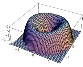
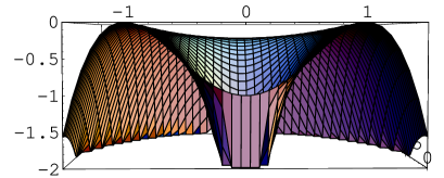
Figure 1: Potential energy $-U^{(A1)}(\phi_{1},\phi_{2})$ in the analogous mechanical system of Model A1: a) Global perspective and b) Section showing the singularity and the $\phi_{2}=0$ path.

depicted in Figure 1. The second summand in the potential energy density $U^{(A1)}(\phi_{1},\phi_{2})$ spoils the $SO(2)$ symmetry preserved by the first summand. The manifold ${\cal M}$ of zeroes of $U^{(A1)}(\phi_{1},\phi_{2})$ is a discrete set of two elements:

$${\cal M}=\{A_{+}=(1,0)\,;\,A_{-}=(-1,0)\}\qquad.$$

The symmetry group of this model is the vierergroup ${\mathbb{G}}=\mathbb{Z}_{2}\times\mathbb{Z}_{2}$ generated by the reflections $\phi_{1}\rightarrow-\phi_{1}$ and $\phi_{2}\rightarrow-\phi_{2}$ in the internal plane. This symmetry is spontaneously broken to the ${\mathbb{Z}}_{2}$ subgroup generated by $\phi_{2}\rightarrow-\phi_{2}$ through the choice of one of the two zeroes, because ${\cal M}$ is the orbit of the other ${\mathbb{Z}}_{2}$ subgroup, in this case generated by $\phi_{1}\rightarrow-\phi_{1}$. The moduli space of zeroes, the quotient space $\bar{\cal M}={\cal M}/{\mathbb{G}}=e$, however, contains only one element $A=\{A_{+},A_{-}\}$.

The partial differential field equations are:

$$\frac{\partial^{2}\phi_{1}}{\partial t^{2}}-\frac{\partial^{2}\phi_{1}}{\partial x^{2}} = 4\phi_{1}\left[1-\phi_{1}^{2}-\phi_{2}^{2}+\frac{\sigma^{2}\phi_{2}^{2}}{(\phi_{1}^{2}+\phi_{2}^{2})^{3}}\right]$$

$$\frac{\partial^{2}\phi_{1}}{\partial t^{2}}-\frac{\partial^{2}\phi_{1}}{\partial x^{2}} = \phi_{2}\left[4-4\phi_{1}^{2}-4\phi_{2}^{2}-\frac{2\sigma^{2}}{(\phi_{1}^{2}+\phi_{2}^{2})^{2}}+\frac{4\sigma^{2}\phi_{2}^{2}}{(\phi_{1}^{2}+\phi_{2}^{2})^{3}}\right]\qquad.$$

In the search for solitary waves, however, we follow the general procedure described in the previous Section because the analogous mechanical system is a Type II Liouville model with:

$$f(R)=(R^{2}-1)^{2}\hskip 56.9055pt,\hskip 56.9055ptg(\varphi)=\sigma^{2}\sin^{2}\varphi\qquad\qquad.$$ (30)

Back in Cartesian coordinates, the superpotential, obtained from the solution of the Hamilton-Jacobi equations, reads:

$$W[\phi_{1},\phi_{2}]=\sqrt{2}\left\{(-1)^{\alpha}\sqrt{\phi_{1}^{2}+\phi_{2}^{2}}\left[\frac{1}{3}(\phi_{1}^{2}+\phi_{2}^{2})-1\right]-(-1)^{\beta}\frac{\sigma\phi_{1}}{\sqrt{\phi_{1}^{2}+\phi_{2}^{2}}}\right\}\qquad.$$

There are no finite action trajectories leaving the area bounded by the circle $C_{1}\equiv\phi_{1}^{2}+\phi_{2}^{2}=1$ of unit radius. Also, finite action trajectories do not cross the radial ray $r_{1}\equiv\phi_{2}=0$; for this reason we call these curves separatrix curves.

3.1 Solitary waves in the boundary of the kink moduli space

From Proposition 1 we know that there exist singular solitary waves whose orbits are $C_{1}$ or $R_{1}$. We use Rajaraman’s trial orbit method in order to identify the form factor of these solitary wave solutions.

$\bullet$ ${\rm K1}_{1}^{AA^{*}}$: Plugging the orbit $C_{1}\equiv\phi_{1}^{2}+\phi_{2}^{2}=1$ into the field equations the following solitary wave solutions are found:

$$\vec{\phi}^{\,\,{\rm K1}_{1}^{AA^{*}}}(x)=\tanh\sqrt{2}\sigma\bar{x}\,\vec{e}_{1}\pm{\rm sech}\sqrt{2}\sigma\bar{x}\,\vec{e}_{2}\qquad.$$ (31)

We refer to them as ${\rm K1}_{1}^{AA^{*}}$ using the notation established in Reference [24]; the subscript stands for the number of lumps that the solitary wave is composed of - see Figure 2- whereas the superscript specifies the elements of ${\cal M}$ that are connected by the kink orbit in a generic way. $A$ can be either $A_{+}$ or $A_{-}$ and by $A^{*}$ we mean the complementary point in ${\cal M}$. In the case depicted in Figure 2, the spatial dependence connects the points $A_{+}$ and $A_{-}$. The density energy and the energy of these kink solutions are respectively

$${\cal E}^{{\rm K1}_{1}^{AA^{*}}}(x)=2\sigma^{2}{\rm sech}^{2}\sqrt{2}\sigma\bar{x}\hskip 28.45274pt,\hskip 28.45274ptE({\rm K1}_{1}^{AA^{*}})=\left|W(A_{-},0)-W(A_{+},0)\right|=2\sqrt{2}\sigma\qquad.$$

In Figure 2 the main features of the solution are depicted for the choice of plus sign in (31) and $\bar{x}=x$: (a) the kink form factor shows that both field components have non-zero profiles. (b) The kink orbits in the internal plane connect the points in ${\cal M}$. (c) The energy density is localized around one point and we interpret these solutions as basic solitary waves. From a physical point of view they are seen as basic traveling particles.

                   

Figure 2: Solitary waves ${\rm K1}_{1}^{AA}$: a) Kink form factor, b) Kink Orbits and c) Energy Density.

$\bullet$ ${\rm K2}_{1}^{AA^{*}}$: Next, the $\phi_{1}$-axis $R_{1}\equiv\phi_{2}=0$ is tried in the ODE system (25). The solution

$$\vec{\phi}^{{\rm K2}_{1}^{AA^{*}}}(x)=\tanh\sqrt{2}\bar{x}\,\vec{e}_{1}$$

corresponds to solitary waves going from $A_{-}$ to $A_{+}$ as $\bar{x}$ varies from $-\infty$ to $+\infty$. Note that these kinks pass through the origin in the internal plane, a very dangerous point. One could surmise that the singularity at this point endows infinity energy to these solutions. We notice, however, that these solutions follow the path $\phi_{2}=0$, where the limit of $w^{(1)}(\phi_{1},\phi_{2})$ is zero, and these kinks do not feel the singularity. In fact, the kink energy density

$${\cal E}^{{\rm K2}_{1}^{AA^{*}}}(x)=2\,{\rm sech}^{4}\sqrt{2}\,\bar{x}$$

$$E({\rm K2}_{1}^{AA^{*}})=\left|W(A_{-},\phi_{2}=0)-\lim_{\varepsilon\rightarrow 0^{-}}W(\varepsilon,\phi_{2}=0)\right|+\left|\lim_{\varepsilon\rightarrow 0^{+}}W(\varepsilon,\phi_{2}=0)-W(A_{+},\phi_{2}=0)\right|=\frac{4\sqrt{2}}{3}$$

is centered around one point in a more concentrated way that the previous solutions - whereas the energy itself is different - and ${\rm K2}_{1}^{AA^{*}}$ kinks belong to another class of basic particles in the model. We emphasize the following subtle point: because $W(\phi_{1},\phi_{2})$ is a regular function all along the $K1_{1}^{AA^{*}}$ kink orbit Stoke’s theorem can be applied and $E[K1_{1}^{AA^{*}}]$ depends only on the value of $W$ at the starting and ending points $A_{\pm}$. The $K2_{1}^{AA^{*}}$ kink orbit, however, hits the origin coming through the $\phi_{2}=0$ axis. The gradient of $W$ is undefined in the neighborhood of the origin along this path and careful application of Stoke’s theorem gives the formula for $E[K2_{1}^{AA^{*}}]$ written above. Note that $E[K1_{1}^{AA^{*}}]\geq E[K2_{1}^{AA^{*}}]$ if $\sigma\geq{2\over 3}$ and $E[K1_{1}^{AA^{*}}]<E[K2_{1}^{AA^{*}}]$ if $\sigma<{2\over 3}$. Figure 3 shows the main features of one of these solitary waves, form factor, orbit and energy density.

In order to gain a deeper understanding of the physical consequences of passing the kink profile through the origin , we shall analyze the stability of ${\rm K2}_{1}^{AA^{*}}$ kinks in some detail. The second-order small fluctuation or Hessian operator around these kinks is the diagonal matrix differential operator

$${\cal H}[{\rm K2}_{1}^{AA^{*}}]=\left(\begin{array}[]{cc}{\cal H}_{11}&{\cal H}_{12}\\ {\cal H}_{21}&{\cal H}_{22}\end{array}\right)=\left(\begin{array}[]{cc}-\frac{d^{2}}{dx^{2}}-4+12\frac{\sinh^{2}\sqrt{2}x}{\cosh^{2}\sqrt{2}x}&0\\ 0&-\frac{d^{2}}{dx^{2}}-4+4\frac{\sinh^{2}\sqrt{2}x}{\cosh^{2}\sqrt{2}x}+2\sigma^{2}\,\frac{{\rm cosh}^{4}\sqrt{2}x}{{\rm sinh}^{4}\sqrt{2}x}\end{array}\right)\,\,.$$

The entry ${\cal H}_{11}$ rules the behavior of the tangent perturbations to the kink orbit. ${\cal H}_{11}$ is an ordinary Schrödinger operator of Posch-Teller type with $\lambda_{0}=0$ as the lowest eigenvalue. The associated eigenfunction (or zero mode) describes a perturbation that is a translation of the kink center, see Figure 3(d). ${\cal H}_{22}$ regulates the orthogonal fluctuations to the $\phi_{2}=0$ orbit. Here, the potential is a positive definite infinite barrier with the singularity at $\bar{x}=0\equiv\vec{\phi}^{{\rm K2}_{1}^{AA^{*}}}(0)=\vec{0}$. This means that fluctuations pushing the kink profile away from the origin cost infinite energy, see Figure 3(d). Therefore, the kink profiles of this kind of solitary waves behave as strings pinned at the origin of the internal plane. In sum, because the spectrum of the Hessian operator is non-negative these solutions are stable. Moreover, ${\rm K1}_{1}^{AA^{*}}$ and ${\rm K2}_{1}^{AA^{*}}$ kinks join the same vacuum points asymptotically and in models without this kind of singularity they would live in the same topological sector of the configuration space. In the present system, however, they belong to different sectors of ${\cal C}$ because they cannot be homotopically deformed into each other under the restriction of finite energy.

     

Figure 3: Solitary waves ${\rm K2}_{1}^{AA}$: a) Kink form factor, b) Kink Orbits, c) Energy Density and d) Potential Well and Barrier in the two diagonal matrix elements of the Hessian operator.

3.2 Solitary waves in the bulk of the kink moduli space

In this model, the Hamilton-Jacobi formulae (19) and (20), or equivalently, the Bogomolny first-order ODE system (28), become :

$$(-1)^{\alpha}\int\,\frac{dR}{R^{2}\,(R^{2}-1)}-(-1)^{\beta}\int\,\frac{d\varphi}{\sigma\,{\rm sin}\,\varphi} = \sqrt{2}$$ (32)

$$\int\,\frac{dR}{R^{2}-1} = \sqrt{2}\bar{x}\qquad.$$ (33)

Integration of (32) gives the kink orbits:

$$\log\left(\left|\frac{R^{K}(x)+1}{R^{K}(x)-1}\right|^{\frac{(-1)^{\alpha}}{2}}\cdot e^{-{1\over R^{K}(x)}}\right)-\log\left|{\rm tan}\frac{\varphi^{K}(x)}{2}\right|^{\frac{(-1)^{\beta}}{\sigma}}=\sqrt{2}\gamma_{1}\qquad.$$ (34)

The kink form factor (kink profile) in the $R$-variable is obtained by integrating (33):

$$R^{K}(x)={\rm tanh}\left(\sqrt{2}\left|\bar{x}\right|\right)\qquad.$$ (35)

Plugging this solution into (32), the kink profile for the angular variable is found:

$$\varphi^{K}(x)=2{\rm arctan}\left[{\rm exp}\left(\sqrt{2}\sigma(\bar{x}+\gamma_{1})-\sigma{\rm cotan}\bar{x}\right)\right]\qquad.$$ (36)

$\bullet$ ${\rm K}_{3}^{AA}(\gamma_{1}^{-},\gamma_{1}^{+})$: In Cartesian coordinates, these solutions -made out of two independent pieces- read:

$$\vec{\phi}^{\,K3^{AO}}(x)=\phi_{1}^{K3^{AO}}(x)\vec{e}_{1}+\phi_{2}^{K3^{AO}}(x)\vec{e}_{2} = -\tanh\sqrt{2}|\bar{x}|\,\tanh\left[\sigma(\sqrt{2}(\bar{x}+\gamma_{1})-{\rm cotanh}\,\sqrt{2}\bar{x})\right]\vec{e}_{1}$$

$$+ \,(-1)^{\alpha}\tanh\sqrt{2}|\bar{x}|\,\,{\rm sech}\left[\sigma(\sqrt{2}(\bar{x}+\gamma_{1})-{\rm cotanh}\,\sqrt{2}\bar{x})\right]\vec{e}_{2}\qquad,$$

starting asymptotically from one of the minima denoted as $A$ and and passing through the origin when $\bar{x}=0$. This point is reached by each member of this family of solutions in such a way that:

$$\lim_{\bar{x}\rightarrow 0^{-}}\frac{d\phi_{1}}{d\bar{x}}=\sqrt{2}\hskip 28.45274pt,\hskip 28.45274pt\lim_{\bar{x}\rightarrow 0^{-}}\frac{d^{n}\phi_{2}}{d\bar{x}^{n}}=0\qquad,\hskip 14.22636ptn=0,1,2,\dots\qquad.$$

This point is crucial, because every solution of this type can be continuously glued with any solution leaving the origin with the same tangency properties and ending at the other point of the vacuum orbit. The whole solution on the real line is thus a kink avoiding the singularity, in the same way as the $K2_{1}^{AA}$ kink does. In sum, there is a two-parametric family of kinks because we can freely choose HJ trajectories with different integration constants $\gamma_{1}^{-}$ and $\gamma_{1}^{+}$ in different regions: $\bar{x}<0$ or $\bar{x}>0$.

A special member of this family is the case when $\bar{\gamma}_{1}=-\infty$:

$$\vec{\phi}^{{\rm K}_{2}^{AA}(\gamma_{1},-\infty)}(x)=\left\{\begin{array}[]{cll}\begin{array}[]{l}-\tanh\sqrt{2}\,|\bar{x}|\,\tanh[\sigma(\sqrt{2}(\bar{x}+\gamma_{1})-{\rm cotanh}\,\sqrt{2}\,\bar{x})]\,\vec{e}_{1}\,+\\ +\,(-1)^{\alpha}\tanh\sqrt{2}\,|\bar{x}|\,\,{\rm sech}[\sigma(\sqrt{2}(\bar{x}+\gamma_{1})-{\rm cotanh}\,\sqrt{2}\,\bar{x})]\,\vec{e}_{2}\end{array}&\mbox{ if }&\bar{x}\leq 0\\[14.22636pt] \tanh\sqrt{2}\,\bar{x}&\mbox{ if }&\bar{x}>0\end{array}\right.\qquad,$$ (37)

which is formed by gluing a kink in the bulk determined by a finite value of $\gamma_{1}^{-}$ at the left of the origin with a kink in the boundary at the right of the origin. Note that for this kind of solution the Hamilton-Jacobi procedure works independently on the left and right half-lines and this is the reason for the dependence on $\gamma_{1}^{-}$ and $\gamma_{1}^{+}$. In Figure 4 we depict the kink field profiles for an $(\gamma_{1}^{-},-\infty)$ orbit with $\bar{x}=0$ and $\alpha=0$. Several kink orbits are also drawn to show that the peculiarity of choosing $\gamma_{1}^{+}=-\infty$ changes the ending point: these kink orbits link the point $A$ of the vacuum orbit with itself by means of a trajectory crossing the origin.

         

Figure 4: Solitary wave family ${\rm K}_{2}^{AA}(\gamma_{1}^{-},-\infty)$: a) Kink form factor and b) Orbits for the values $\gamma_{1}^{-}=0,\pm 1,\pm 2$.

Moreover, a Mathematica plot of the energy density for several values of $\gamma_{1}^{-}$ (see Figure 5) shows that these solutions are indeed a non-linear superposition of the basic solitary waves discussed above: one ${\rm K1}_{1}^{AA}$ kink plus one ${\rm K2}_{1}^{AA}$ kink. Observe, however, that the solutions parametrized by $\gamma_{1}^{-}$ are composed of one $K1_{1}^{AA}$ and one-half $K2_{1}^{AA}$ kinks whereas the choice of $\gamma_{1}^{+}=-\infty$ continuously glues the remaining one-half $K2_{1}^{AA}$ kink. This justifies the nomenclature ${\rm K}_{2}^{AA}(\gamma_{1}^{-},-\infty)$ for this kink family. If $\gamma_{1}^{-}$ is positive, these solutions behave as two separate lumps whereas if $\gamma_{1}^{-}$ is negative the two lumps sit on top of each other.

Figure 5: Energy density of the ${\rm K}_{2}^{AA}(\gamma_{1},-\infty)$ solitary waves for decreasing values of $\gamma_{1}^{-}$.

The energy of these solutions is evaluated using expression (6) to find: $E[{\rm K}_{2}^{AA}(\gamma_{1}^{-},-\infty)]=\frac{4\sqrt{2}}{3}+2\sqrt{2}\sigma$. The following kink energy sum rule

$$E[{\rm K}_{2}^{AA}(\gamma_{1}^{-},-\infty)]=E[{\rm K1}_{1}^{AA}]+E[{\rm K2}_{1}^{AA}]$$

holds, showing the composite character of these solitary waves built from two basic kinks.

Fully general solutions have the form:

$$\vec{\phi}^{{\rm K}_{3}^{AA^{*}}(\gamma_{1}^{+},\gamma_{1}^{-})}(x)=\left\{\begin{array}[]{l}\phi_{1}^{K_{3}^{AO}}(\bar{x};\gamma_{1}^{-})\,\vec{e}_{1}+\phi_{2}^{K_{3}^{AO}}(\bar{x};\gamma_{1}^{-})\,\vec{e}_{2}\mbox{ if }\bar{x}\leq 0\\ \phi_{1}^{K_{3}^{AO}}(\bar{x};\gamma_{1}^{+})\,\vec{e}_{1}-\phi_{2}^{K_{3}^{AO}}(\bar{x};\gamma_{1}^{+})\,\vec{e}_{2}\mbox{ if }\bar{x}>0\end{array}\right.\qquad.$$

Their energy density is the sum of two ${\rm K1}_{1}^{AA}$ and one ${\rm K2}_{1}^{AA}$ lumps, and is therefore a composite of three basic kinks:

$$E[{\rm K}_{3}^{AA^{*}}]=2E[{\rm K1}_{1}^{AA^{*}}]+E[{\rm K2}_{1}^{AA^{*}}]=4\sqrt{2}\sigma+\frac{4\sqrt{2}}{3}$$

         

Figure 6: Several $K_{3}^{AA}(\gamma_{1}^{+},\gamma_{1}^{-})$ kink orbits

A short remark on stability: $K_{2}^{AA}(\gamma_{1}^{-},-\infty)$ solitary waves are non-topological whereas the $K_{3}^{AA}(\gamma_{1}^{-},\gamma_{1}^{+}))$ family is formed by topological kinks. Both types, however, are stable because, passing through the origin, they cannot decay to lighter kinks with the same asymptotic behavior for identical reasons that forbid the decay of the $K2_{1}^{AA}$ to the $K1_{1}^{AA}$ kink.

4 The B1 Model

In this section we study the deformation induced on the potential $v^{(B)}(\phi_{1},\phi_{2})$ (4) by $w^{(1)}(\phi_{1},\phi_{2})$ (8). The dynamics is governed by the action functional (5), with potential energy density:

$$U^{(B1)}(\phi_{1},\phi_{2})=(\phi_{1}^{2}+\phi_{2}^{2}-1)^{2}(\phi_{1}^{2}+\phi_{2}^{2}-a^{2})^{2}+\frac{\sigma^{2}\phi_{2}^{2}}{(\phi_{1}^{2}+\phi_{2}^{2})^{2}}\qquad.$$

Thus, as in the $A1$ model, by adding the $w^{(1)}$ perturbation the symmetry under the $SO(2)$ group is explicitly broken to the discrete subgroup ${\mathbb{G}}=\mathbb{Z}_{2}\times\mathbb{Z}_{2}$ generated by reflections of the fields: $\phi_{1}\rightarrow-\phi_{1}$, $\phi_{2}\rightarrow-\phi_{2}$.

For the sake of simplicity we set the value of $a$ to be: $a=2$. Other non-null values of this parameter yield the same qualitative behavior of the system with only analytic differences in the specific expressions. The set of zeroes of $v^{(B)}(\phi_{1},\phi_{2})$ is a continuous manifold with two connected components: the disjoint union of two circles of radius $1$ and $2$, $S^{1}_{r=1}\cup S^{1}_{r=2}$. The $w^{1}$ perturbation, however, forces the set of zeroes of $U^{(B1)}$ to be the discrete set of four points:

$${\cal M}=\{B^{-}=(-2,0)\,\,;\,\,A^{-}=(-1,0)\,\,;\,\,A^{+}=(1,0)\,\,;\,\,B^{+}=(2,0)\}\qquad.$$

The vacuum orbit is the union of two ${\mathbb{G}}$-orbits: ${\cal M}=\{A^{-},A^{+}\}\cup\{B^{-},B^{+}\}$. The moduli space of vacua $\bar{\cal M}={\cal M}/{\mathbb{G}}=A\cup B$, however, is the union of only two elements: $A=\{A^{-},A^{+}\}$, $B=\{B^{-},B^{+}\}$.

The field equations are:

$$\frac{\partial^{2}\phi_{1}}{\partial t^{2}}-\frac{\partial^{2}\phi_{1}}{\partial x^{2}} = 4\phi_{1}\left[(1-\phi_{1}^{2}-\phi_{2}^{2})(4-\phi_{1}^{2}-\phi_{2}^{2})(5-2\phi_{1}^{2}-2\phi_{2}^{2})+\frac{\sigma^{2}\phi_{2}^{2}}{(\phi_{1}^{2}+\phi_{2}^{2})^{3}}\right]$$

$$\frac{\partial^{2}\phi_{2}}{\partial t^{2}}-\frac{\partial^{2}\phi_{2}}{\partial x^{2}} = 4\phi_{2}\left[(1-\phi_{1}^{2}-\phi_{2}^{2})(4-\phi_{1}^{2}-\phi_{2}^{2})(5-2\phi_{1}^{2}-2\phi_{2}^{2})-\frac{\sigma^{2}}{2(\phi_{1}^{2}+\phi_{2}^{2})^{2}}+\frac{\sigma^{2}\phi_{2}^{2}}{(\phi_{1}^{2}+\phi_{2}^{2})^{3}}\right]\qquad.$$

The analogous mechanical system is the Type II Liouville system for which:

$$f(R)=(1-R^{2})^{2}(4-R^{2})^{2}\hskip 56.9055pt,\hskip 56.9055ptg(\varphi)=\sigma^{2}\sin^{2}\varphi\qquad.$$

Back in Cartesian coordinates, the superpotentials, obtained from the solution of the Hamilton-Jacobi equation, read:

$$W[\phi_{1},\phi_{2}]=\sqrt{2}\left\{(-1)^{\alpha}\sqrt{\phi_{1}^{2}+\phi_{2}^{2}}\left[\frac{1}{5}(\phi_{1}^{2}+\phi_{2}^{2})^{2}-\frac{1+a^{2}}{3}(\phi_{1}^{2}+\phi_{2}^{2})+a^{2}\right]-(-1)^{\beta}\frac{\sigma\phi_{1}}{\sqrt{\phi_{1}^{2}+\phi_{2}^{2}}}\right\}\qquad.$$

There are no finite action trajectories trespassing the circle: $C_{2}\equiv\phi_{1}^{2}+\phi_{2}^{2}=4$. Also, $C_{1}\equiv\phi_{1}^{2}+\phi_{2}^{2}=1$, and $R_{1}\equiv\phi_{2}=0$ are not crossed by any finite-action trajectories. Thus, $C_{1}$, $C_{2}$, and $R_{1}$ form the set of separatrix curves of the $B1$ model.

4.1 Solitary waves at the boundary of the moduli space

From Proposition 1 in section §2, the existence of singular solitary waves with $C_{2}$, $C_{1}$, and $R_{1}$ orbits follows. Use of the Rajaraman s trial orbit method is effective.

$\bullet$ $K1_{1}^{AA^{*}}$. Substituting $\phi_{1}^{2}+\phi_{2}^{2}=1$ into (28) we obtain the following solitary wave solutions:

$$\vec{\phi}^{\,{\rm K1}_{1}^{AA^{*}}}(x)=\tanh\sqrt{2}\sigma\bar{x}\,\vec{e}_{1}\pm\,{\rm sech}\sqrt{2}\sigma\bar{x}\,\vec{e}_{2}\qquad,$$

joining the points $A_{+}$ and $A_{-}$, see Figure 7. They are basic lumps or particles of the $B1$ model - recall that exactly the same solutions are also solutions of model $A1$- and their energy density is concentrated around a point in the real line, see Figure 7c. Specifically, we find that the energy density and the energy of these kinks is exactly the same as in model $A1$:

$${\cal E}^{{\rm K1}_{1}^{AA^{*}}}(x)=2\sigma^{2}{\rm sech}^{2}\sqrt{2}\sigma\bar{x}\hskip 28.45274pt,\hskip 28.45274ptE[{\rm K1}_{1}^{AA^{*}}]=\left|W(A_{-},0)-W(A_{+},0)\right|=2\sqrt{2}\sigma\qquad.$$

                   

Figure 7: Solitary waves ${\rm K1}_{1}^{AA^{*}}$: a) Factor Form, b) Orbit and c) Energy Density.

$\bullet$ $K_{1}^{BB^{*}}$. Analogously, we choose $\phi_{1}^{2}+\phi_{2}^{2}=4$ as the trial orbit and plug this expression into (28), to obtain:

$$\vec{\phi}^{\,{\rm K}_{1}^{BB^{*}}}(x)=2\tanh\frac{\sigma\bar{x}}{2\sqrt{2}}\,\vec{e}_{1}+2\,{\rm sech}\frac{\sigma\bar{x}}{2\sqrt{2}}\,\vec{e}_{2}\qquad.$$

These solitary waves share similar features with the $K_{1}^{AA^{*}}$ kinks, although in this case the asymptotically linked points are $B_{+}$ and $B_{-}$. Even though the total amount of energy carried out by the ${\rm K}_{1}^{BB^{*}}$ and ${\rm K1}_{1}^{AA^{*}}$ kinks is the same, the energy density is less concentrated in the ${\rm K}_{1}^{BB^{*}}$ kinks:

$${\cal E}^{{\rm K1}_{1}^{BB^{*}}}(x)={\sigma^{2}\over 2}{\rm sech}^{2}{\sigma\bar{x}\over 2\sqrt{2}}\hskip 28.45274pt,\hskip 28.45274ptE[{\rm K1}_{1}^{BB^{*}}]=\left|W(B_{-},0)-W(B_{+},0)\right|=2\sqrt{2}\sigma\qquad,$$

see Figure 8. They describe different basic particles, living in different topological sectors.

                   

Figure 8: Solitary waves ${\rm K}_{1}^{BB^{*}}$: a) Factor Form, b) Orbit and c) Energy Density.

On the $\phi_{2}=0$ axis there are two different kinds of singular solitary waves.

$\bullet$ $K_{1}^{AB}$: The first kind includes two kink orbits, the closed intervals $[B_{-},A_{-}]$ -$\aleph=1$- and $[A_{+},B_{+}]$ -$\aleph=0$-. The corresponding kinks connect points in different elements $A$ and $B$ of the vacuum moduli space. We denote this kind of solitary wave solutions as $K_{1}^{AB}$ kinks and their profiles or form factors are easily found to be:

$$\vec{\phi}^{\,{\rm K}_{1}^{AB}}(x)=2\cos\left[\frac{2}{3}\arctan e^{6\sqrt{2}\bar{x}}+\frac{2\pi}{3}\aleph\right]\vec{e}_{1}\qquad,\qquad\aleph=0,1$$

The energy density and total energy of these solutions is:

$${\cal E}^{{\rm K}_{1}^{AB}}(x)=32\,{\rm sech}^{2}6\sqrt{2}\bar{x}\,\sin^{2}\left(\frac{2}{3}\arctan e^{6\sqrt{2}\bar{x}}+{2\pi\over 3}\aleph\right)$$

$$E[{\rm K}_{1}^{AB}]=\left|W(A_{\mp},0)-W(B_{\mp},0)\right|=\frac{22\sqrt{2}}{15}\qquad.$$

The energy density is again localized around a point and these solutions are also basic solitary waves or lumps of the $B1$ model, see Figure 9.

                   

Figure 9: Solitary waves ${\rm K}_{1}^{AB}$: a) Form Factor b) Orbit and c) Energy Density.

$\bullet$ $K2_{1}^{AA^{*}}$: The orbit of the second kind of solitary waves on the $\phi_{2}$ axis is the $[A_{-},A_{+}]$ interval. The kink profile of these kinks connects these points in the vacuum orbit and is also easy to determine:

$$\vec{\phi}^{{\rm K2}_{1}^{AA^{*}}}(x)=2\cos\left[\frac{2}{3}\arctan e^{6\sqrt{2}\bar{x}}+\frac{4\pi}{3}\right]\vec{e}_{1}\qquad.$$

Despite being analytically different, the behavior of these kinks is completely analogous to that of the bizarre $K2_{1}^{AA^{*}}$ solitary waves of the A1 model. The energy density and total energy of these kinks are:

$${\cal E}^{{\rm K2}_{1}^{AA^{*}}}(x)=32\,{\rm sech}^{2}6\sqrt{2}\bar{x}\,\sin^{2}\left(\frac{2}{3}\arctan e^{6\sqrt{2}\bar{x}}+{4\pi\over 3}\right)$$

$$E[{\rm K2}_{1}^{AA^{*}}]=\left|W(A_{-},\phi_{2}=0)-\lim_{\varepsilon\rightarrow 0^{-}}W(\varepsilon,\phi_{2}=0)\right|+\left|\lim_{\varepsilon\rightarrow 0^{+}}W(\varepsilon,\phi_{2}=0)-W(A_{+},\phi_{2}=0)\right|=\frac{76\sqrt{2}}{15}\qquad,$$

see Figure 3 to find qualitative plots of their properties.

4.2 Solitary waves in the bulk of the moduli space

The Hamilton-Jacobi orbit (19) and time schedule (20) are in this case the quadratures:

$$(-1)^{\alpha}\int\frac{dR}{R^{2}(1-R^{2})(4-R^{2})}-(-1)^{\beta}\int\frac{d\varphi}{\sigma\sin\varphi} = \sqrt{2}\gamma_{1}$$

$$\int\frac{dR}{(1-R^{2})(4-R^{2})} = \sqrt{2}\bar{x}\qquad.$$

Integration of these equations provides the analytic expressions for kink orbits and form factors:

$$(-1)^{\alpha}\left[\frac{-1}{4R}+\frac{1}{6}\log\frac{(R-2)^{\frac{1}{8}}(R+1)}{(R+2)^{\frac{1}{8}}(R-1)}\right]-\frac{(-1)^{\beta}}{\sigma}\log\tan\frac{\varphi}{2} = \sqrt{2}\gamma_{1}$$ (38)

$$\frac{1}{12}\log\frac{(R-2)(R+1)^{2}}{(R+2)(R-1)^{2}} = \sqrt{2}\bar{x}\qquad.$$ (39)

Solitary wave solutions only arise from equations (38) and (39) if $1\leq R\leq 2$ or $0\leq R\leq 1$. Let us denote $\Theta=\arctan e^{6\sqrt{2}\bar{x}}+{2\pi\over 3}\aleph$ in the first range, $\Theta=\arctan e^{6\sqrt{2}\bar{x}}+{4\pi\over 3}$ in the second range, and let us define the functions:

$$\Omega_{1}(x)=\frac{\cos\frac{2\Theta}{3}+\frac{1}{2}}{\cos\frac{2\Theta}{3}-\frac{1}{2}}\hskip 19.91684pt;\hskip 19.91684pt\Omega_{2}(x)=\frac{\Omega_{1}(x)-1}{\Omega_{1}(x)+1}=\frac{1}{2}\sec\frac{2\Theta}{3}\hskip 19.91684pt;\hskip 19.91684pt\Lambda(x)=\tan\frac{\Theta}{3}\qquad.$$ (40)

$\bullet$ ${\rm K}_{2}^{AB}(\gamma_{1})$: If $1\leq R\leq 2$, the solutions in Cartesian coordinates are:

$$\vec{\phi}^{{\rm K}_{2}^{AB}(\gamma_{1})}(x)=\phi_{1}^{{\rm K}_{2}^{AB}(\gamma_{1})}(x)\,\vec{e}_{1}+\phi_{2}^{{\rm K}_{2}^{AB}(\gamma_{1})}(x)\,\vec{e}_{2}$$

$$\vec{\phi}^{{\rm K}_{2}^{AB}(\gamma_{1})}(x) = \frac{1}{\Omega_{2}(\bar{x})}\left[\frac{2}{1+e^{-2\sqrt{2}\sigma\gamma_{1}}\,e^{-\frac{\sigma}{2}\Omega_{2}(\bar{x})}\,\Omega_{1}^{\frac{\sigma}{3}}(\bar{x})\,\Lambda^{\frac{\sigma}{12}}(\bar{x})}-1\right]\vec{e}_{1}$$

$$+ (-1)^{\alpha}\,\frac{2\,e^{\sqrt{2}\sigma\gamma_{1}}\,e^{\frac{\sigma}{4}\Omega_{2}(\bar{x})}\,\Omega_{1}^{\frac{\sigma}{6}}(\bar{x})\,\Lambda^{\frac{\sigma}{24}}(\bar{x})}{\Omega_{2}(\bar{x})\left(e^{2\sqrt{2}\sigma\gamma_{1}}\,e^{\frac{\sigma}{2}\Omega_{2}(\bar{x})}+\Omega_{1}^{\frac{\sigma}{3}}(\bar{x})\,\Lambda^{\frac{\sigma}{12}}(\bar{x})\right)}\vec{e}_{2}\qquad,\qquad\alpha=0,1\qquad.$$

The kink orbits belonging to these two one-parametric families connect either $A_{-}$ to $B_{+}$ if $\aleph=0$, or $A_{+}$ to $B_{-}$ if $\aleph=0$, and are confined inside the annulus bounded by the circles $C_{1}$ and $C_{2}$, see Figure 10. The energy density of each member of these kink families is localized around two distinct points, see Figure 10. For sufficiently negative, values of $\gamma_{1}$ the two lumps are composed of one $K1_{1}^{AA^{*}}$ and one $K_{1}^{AB}$ basic kinks. In the opposite regime, for sufficiently positive values of $\gamma_{1}$, two lumps arise again, close to one $K_{1}^{BB^{*}}$ and one $K_{1}^{AB}$ basic kinks. Note that the basic kinks appear at the boundary of the moduli space when either $\gamma_{1}=-\infty$ or $\gamma_{1}=\infty$. Intermediate tuning of $\gamma_{1}$ continuously shifts from one configuration to the other, see Figure 11. These features are synthesized in the notation ${\rm K}_{2}^{AB}(\gamma_{1})$.

         

Figure 10: Solitary wave family ${\rm K}_{2}^{AB}(\gamma_{1})$: a) form factor and b) Orbits for values $\gamma_{1}=0,\pm 1,\pm 2$.

Figure 11: Energy Density of the solitary wave family ${\rm K}_{2}^{AB}(\gamma_{1})$ for increasing values of $\gamma_{1}$.

$\bullet$ ${\rm K}_{3}^{AA}(\gamma_{1}^{+},\gamma_{1}^{-})$: Inside the $C_{1}$, $0<R<1$, there are kink solutions completely analogous to the ${\rm K}_{3}^{AA}(\gamma_{1}^{+},\gamma_{1}^{-})$ solitary waves of the $A1$ model, see Figure 6. The kink profiles have the form:

$$\vec{\phi}^{{\rm K}_{3}^{AA^{*}}(\gamma_{1}^{+},\gamma_{1}^{-})}(x)=\left\{\begin{array}[]{l}\phi_{1}^{K_{3}^{AO}}(\bar{x};\gamma_{1}^{-})\,\vec{e}_{1}+\phi_{2}^{K_{3}^{AO}}(\bar{x};\gamma_{1}^{-})\,\vec{e}_{2}\mbox{ if }\bar{x}\leq 0\\ \phi_{1}^{K_{3}^{AO}}(\bar{x};\gamma_{1}^{+})\,\vec{e}_{1}-\phi_{2}^{K_{3}^{AO}}(\bar{x};\gamma_{1}^{+})\,\vec{e}_{2}\mbox{ if }\bar{x}>0\end{array}\right.\qquad,$$

where

$$\vec{\phi}^{{\rm K}_{2}^{AO}(\gamma_{1})}(x) = \frac{1}{\Omega_{2}(\bar{x})}\left[\frac{2}{1+e^{-2\sqrt{2}\sigma\gamma_{1}}\,e^{-\frac{\sigma}{2}\Omega_{2}(\bar{x})}\,\Omega_{1}^{\frac{\sigma}{3}}(\bar{x})\,\Lambda^{\frac{\sigma}{12}}(\bar{x})}-1\right]\vec{e}_{1}$$

$$+ (-1)^{\alpha}\,\frac{2\,e^{\sqrt{2}\sigma\gamma_{1}}\,e^{\frac{\sigma}{4}\Omega_{2}(\bar{x})}\,\Omega_{1}^{\frac{\sigma}{6}}(\bar{x})\,\Lambda^{\frac{\sigma}{24}}(\bar{x})}{\Omega_{2}(\bar{x})\left(e^{2\sqrt{2}\sigma\gamma_{1}}\,e^{\frac{\sigma}{2}\Omega_{2}(\bar{x})}+\Omega_{1}^{\frac{\sigma}{3}}(\bar{x})\,\Lambda^{\frac{\sigma}{12}}(\bar{x})\right)}\vec{e}_{2}\qquad,\qquad\alpha=0,1\qquad,$$

and $\Theta=\arctan e^{6\sqrt{2}\bar{x}}+{4\pi\over 3}$ in the $0<R<1$ range.

In particular , the limiting case $K_{3}^{AA}(\gamma_{1}^{+},-\infty)$ gives a solitary wave identical to the $K_{2}^{AA}(\gamma_{1})$ kink of the A1 model. To obtain the kink profile one replaces $\phi_{1}^{K_{3}^{AO}}(\bar{x};\gamma_{1}^{-})\,\vec{e}_{1}+\phi_{2}^{K_{3}^{AO}}(\bar{x};\gamma_{1}^{-})\,\vec{e}_{2}$ by $\vec{\phi}^{K2_{1}^{AA^{*}}}(\gamma_{1})(x)=2{\rm cos}\Theta\vec{e}_{1}$ on the left ($\bar{x}<0$). We recall that these solutions connect a point in $A$ with itself through a trajectory that crosses the origin, see Figure 4.

In sum, the structure of the solitary wave variety in the B1 model is as follows: There exist four kinds of basic lumps associated with the ${\rm K1}_{1}^{AA^{*}}$, ${\rm K2}_{1}^{AA^{*}}$, ${\rm K}_{1}^{BB}$ and ${\rm K}_{1}^{AB}$ kinks, which display different distributions of one-point localized energy densities. The ${\rm K}_{3}^{AA}(\gamma_{1}^{+},\gamma_{1}^{-}))$, ${\rm K}_{2}^{AA}(\gamma_{1})$, and ${\rm K}_{2}^{AB}(\gamma_{1})$ kinks, however, are composite solitary waves. The ${\rm K}_{3}^{AA}(\gamma_{1}^{+},\gamma_{1}^{-})$ kinks are combinations of two ${\rm K1}_{1}^{AA^{*}}$ and one ${\rm K2}_{1}^{AA^{*}}$ basic lumps; the ${\rm K}_{2}^{AA}(\gamma_{1})$ are formed by one ${\rm K1}_{1}^{AA^{*}}$ and one ${\rm K2}_{1}^{AA^{*}}$ basic lumps, the ${\rm K}_{2}^{AB}(\gamma_{1})$ kinks exhibit an orbit dependent structure that varies between the limiting combination formed by either the ${\rm K1}_{1}^{AA^{*}}$ and ${\rm K}_{1}^{AB}$ kinks or the ${\rm K1}_{1}^{BB^{*}}$ and ${\rm K}_{1}^{AB}$ kinks. Therefore, the following kink energy sum rules hold:

$$E[K_{3}^{AA}]=2E[K1_{1}^{AA}]+E[K2_{1}^{AA}]=4\sqrt{2}\sigma+{76\over 15}\sqrt{2}$$

$$E[K_{2}^{AA}]=E[K1_{1}^{AA}]+E[K2_{1}^{AA}]=2\sqrt{2}\sigma+{76\over 15}\sqrt{2}$$

$$E[K_{2}^{AB}]=E[K_{1}^{AB}]+E[K_{1}^{BB}]=E[K_{1}^{AB}]+E[K1_{1}^{AA}]=2\sqrt{2}\sigma+{22\over 15}\sqrt{2}\qquad.$$

With respect to stability, all the kinks inside the $C_{1}$ circle behave like their cousins in the A1 model. All the kinks in the $1\leq R\leq 2$ annulus are stable.

5 The A2 model

In this Section we analyze the deformation induced on the potential $v^{(A)}(\phi_{1},\phi_{2})$ (3) by $w^{(2)}(\phi_{1},\phi_{2})$ (9). The action functional (5) with potential energy

$$U_{\rm A2}(\phi_{1},\phi_{2})=(\phi_{1}^{2}+\phi_{2}^{2}-1)^{2}+\frac{\sigma^{2}}{2(\phi_{1}^{2}+\phi_{2}^{2})}\left(1-\frac{\phi_{1}}{\sqrt{\phi_{1}^{2}+\phi_{2}^{2}}}\right)$$ (41)

governs the dynamics. This deformation explicitly breaks the $SO(2)$ symmetry to the discrete group $\mathbb{Z}_{2}$ generated by the reflection $\phi_{2}\rightarrow-\phi_{2}$. The set ${\cal M}$ of zeroes of $U(\phi_{1},\phi_{2})$ has only one element:

$${\cal M}=\{\,A=(1,0)\,\}\qquad\qquad.$$

In this model, the second order partial differential equations

$$\frac{\partial^{2}\phi_{1}}{\partial t^{2}}-\frac{\partial^{2}\phi_{1}}{\partial x^{2}} = 4\phi_{1}(1-\phi_{1}^{2}-\phi_{2}^{2})+\frac{\sigma^{2}}{2}\frac{\phi_{2}^{2}-2\phi_{1}^{2}+2\phi_{1}\sqrt{\phi_{1}^{2}+\phi_{2}^{2}}}{(\phi_{1}^{2}+\phi_{2}^{2})^{\frac{5}{2}}}$$

$$\frac{\partial^{2}\phi_{1}}{\partial t^{2}}-\frac{\partial^{2}\phi_{1}}{\partial x^{2}} = 4\phi_{2}(1-\phi_{1}^{2}-\phi_{2}^{2})+\frac{\sigma^{2}}{2}\left[\frac{2\phi_{2}}{(\phi_{1}^{2}+\phi_{2}^{2})^{2}}-\frac{3\phi_{1}\phi_{2}}{(\phi_{1}^{2}+\phi_{2}^{2})^{\frac{5}{2}}}\right]$$

are the field equations. The asymptotic conditions (7) guaranteeing finite energy compel the solitary wave solutions to link the only minimum $A$ with itself. The general results in Section §. 2 ensure that the $C_{1}\equiv\phi_{1}^{2}+\phi_{2}^{2}=1$ circle and the $r_{1}\equiv\,\phi_{2}=0\,\cup\,\phi_{1}>0$ abscissa half axis are separatrix curves. Unlike the A1 and B1 models (see Section §. 3 and §. 4) the singularity at the origin is of different nature in this case. We know from previous Sections that there exists a path $\phi_{2}=0$ along which the singularity is not felt in either model A1 or B1. The potential energy $U^{\rm A2}(\phi_{1},\phi_{2})$, however, reduces on the abscissa axis to:

$$U^{\rm A2}(\phi_{1},0)=(\phi_{1}^{2}-1)^{2}+\frac{\sigma^{2}}{2\phi_{1}^{2}}\left(1-\,{\rm sign}\,(\phi_{1})\right)$$

and the singularity is always felt in the $\phi_{1}<0$ negative half-axis. There is no escape to kink orbits that enter through the positive abscissa half-axis, and finite energy solitary waves are pushed away from the origin.

Nevertheless, there are kink orbits on the $C_{1}\equiv\phi_{1}^{2}+\phi_{2}^{2}=1$ circle.

$\bullet$ ${\rm K}_{1}^{AA}$: Plugging this curve into (28) we obtain

$$\vec{\phi}^{{\rm K}_{1}^{AA}}(x)=\left(2\tanh^{2}\frac{\sigma\bar{x}}{\sqrt{2}}-1\right)\vec{e}_{1}+2\,{\rm sech}\,\frac{\sigma\bar{x}}{\sqrt{2}}\tanh\frac{\sigma\bar{x}}{\sqrt{2}}\,\,\vec{e}_{2}\qquad,$$

a solitary wave connecting the point $A$ with itself when $x$ varies from $-\infty$ to $\infty$, see Figure 12(a,b). The energy density

$${\cal E}^{{\rm K}_{1}^{AA}}(x)=2\,\sigma^{2}\,{\rm sech}^{2}\,\frac{\sigma\bar{x}}{\sqrt{2}}\hskip 56.9055pt,\hskip 56.9055ptE[{\rm K}_{1}^{AA}]=4\sqrt{2}\sigma$$

is localized at one point so that the ${\rm K}_{1}^{AA}$ is a basic lump, see Figure 12(c).

                   

Figure 12: Solitary waves ${\rm K}_{1}^{AA}$: a) Factor Form, b) Orbit and c) Energy Density.

Again we are dealing with a mechanical analogous system of Liouville Type II such that:

$$f(R)=(R^{2}-1)^{2}\hskip 56.9055pt,\hskip 56.9055ptg(\varphi)=\sigma^{2}\sin^{2}\frac{\varphi}{2}\qquad.$$

In Cartesian coordinates the superpotentials read:

$$\left\{\begin{array}[]{c}W^{+}(\phi_{1},\phi_{2})=(-1)^{\alpha}\sqrt{2}\sqrt{\phi_{1}^{2}+\phi_{2}^{2}}\left(\frac{\phi_{1}^{2}+\phi_{2}^{2}}{3}-1\right)-2\sigma(-1)^{\beta}\sqrt{1+\sqrt{\frac{\phi_{1}^{2}}{\phi_{1}^{2}+\phi_{2}^{2}}}}\qquad,\qquad\phi_{2}>0\\ W^{-}(\phi_{1},\phi_{2})=(-1)^{\alpha}\sqrt{2}\sqrt{\phi_{1}^{2}+\phi_{2}^{2}}\left(\frac{\phi_{1}^{2}+\phi_{2}^{2}}{3}-1\right)+2\sigma(-1)^{\beta}\sqrt{1+\sqrt{\frac{\phi_{1}^{2}}{\phi_{1}^{2}+\phi_{2}^{2}}}}\qquad,\qquad\phi_{2}<0\end{array}\right.$$

and we realize that the kink energy is a topological bound

$$E[{\rm K}_{1}^{AA}]=\left|W^{+}(A)-W^{-}(A)\right|=4\sqrt{2}\sigma$$

giving the winding number of the kink orbit around the origin. This fact ensures stability for the ${\rm K}_{1}^{AA}$ kink.

The Hamilton-Jacobi theory yields the remaining solutions confined inside the unit circle $C_{1}$. In this model, the Hamilton-Jacobi formulae (19) and (20) or, equivalently, the Bogomolny first-order ODE system (28) become:

$$(-1)^{\alpha}\int\,\frac{dR}{R^{2}\,(R^{2}-1)}-(-1)^{\beta}\int\,\frac{d\varphi}{{2}\sqrt{\sigma}\,{\rm sin}\,{\varphi\over 2}} = \sqrt{2}\gamma_{1}$$ (42)

$$\int\,\frac{dR}{R^{2}-1} = \sqrt{2}\bar{x}\qquad.$$ (43)

Integration of (42) gives the kink orbits:

$$\log\left(\left|\frac{R^{K}(x)+1}{R^{K}(x)-1}\right|^{\frac{(-1)^{\alpha}}{2}}\cdot e^{-{1\over R^{K}(x)}}\right)-\log\left|{\rm tan}\frac{\varphi^{K}(x)}{4}\right|^{\frac{(-1)^{\beta}}{\sigma}}=\sqrt{2}\gamma_{1}\qquad.$$ (44)

The kink form factor (kink profile) in the $R$-variable is obtained by integrating (43):

$$R^{K}(x)={\rm tanh}\left(\sqrt{2}\left|\bar{x}\right|\right)\qquad.$$ (45)

Plugging this solution into (42) the kink profile for the angular variable is found:

$$\varphi^{K}(x)=4{\rm arctan}\left[{\rm exp}\left(\sqrt{2}\sigma(\bar{x}+\gamma_{1})-\sigma{\rm cotan}\sqrt{2}\bar{x}\right)\right]\qquad.$$ (46)

Back in Cartesian coordinates, we obtain:

$$\vec{\phi}(x) = \tanh\sqrt{2}|\bar{x}|\left\{1-2\,{\rm sech}\,\left[\frac{\sigma}{2}\left(\gamma_{1}-\sqrt{2}\bar{x}+{\rm cotanh}\,\sqrt{2}\bar{x}\right)\right]\right\}\vec{e}_{1}+$$

$$+ 2\tanh\sqrt{2}|\bar{x}|\tanh\left(\gamma_{1}-\sqrt{2}\bar{x}+{\rm cotanh}\,\sqrt{2}\bar{x}\right){\rm sech}\left(\gamma_{1}-\sqrt{2}\bar{x}+{\rm cotanh}\,\sqrt{2}\bar{x}\right)\vec{e}_{2}\qquad.$$

Some orbits for these solutions are depicted in Figure 13. Here, we notice that all solutions of this kind head towards the origin; thus, they cannot be regarded as finite-energy solutions.

Figure 13: Trajectories of solutions confined in the unit circle $C_{1}$.

In sum, in model $A2$ there exists only one basic solitary wave, the ${\rm K}_{1}^{AA}$ kink, and no composite solitary waves arise.

6 The B2 Model

Finally, in this last section we study the deformation $w^{(2)}$ (9) induced on $v^{(B)}$ (4). Therefore, the potential term

$$U_{\rm B2}(\phi_{1},\phi_{2})=(\phi_{1}^{2}+\phi_{2}^{2}-1)^{2}(\phi_{1}^{2}+\phi_{2}^{2}-a^{2})^{2}+\frac{\sigma^{2}}{2(\phi_{1}^{2}+\phi_{2}^{2})}\left(1-\frac{\phi_{1}}{\sqrt{\phi_{1}^{2}+\phi_{2}^{2}}}\right)$$ (47)

enters the functional action (5). We set the $a=2$ value bearing in mind that models of B2 type characterized by other non-null values of the parameter $a$ show a very similar behavior. As in the $A2$ model, the second summand on the right hand side of (47) explicitly breaks the $SO(2)$ symmetry of the unperturbed system (4) to the discrete group $\mathbb{Z}_{2}$ generated by the $\phi_{2}\rightarrow-\phi_{2}$ reflection. The non-deformed manifold of zeroes ${\cal M}_{\sigma=0}=S^{1}_{r=1}\cup S^{1}_{r=2}$, the disjoint union of two circles, becomes the discrete set of two elements:

$${\cal M}=\{\,A=(1,0)\,\,;\,\,B=(2,0)\}\qquad\qquad.$$

The Euler-Lagrange equations form the system of second-order PDEs:

$$\frac{\partial^{2}\phi_{1}}{\partial t^{2}}-\frac{\partial^{2}\phi_{1}}{\partial x^{2}} = 4\phi_{1}(1-\phi_{1}^{2}-\phi_{2}^{2})(4-\phi_{1}^{2}-\phi_{2}^{2})(5-2\phi_{2}^{2}-2\phi_{2}^{2})+\frac{\sigma^{2}}{2}\frac{\phi_{2}^{2}-2\phi_{1}^{2}+2\phi_{1}\sqrt{\phi_{1}^{2}+\phi_{2}^{2}}}{(\phi_{1}^{2}+\phi_{2}^{2})^{\frac{5}{2}}}$$

$$\frac{\partial^{2}\phi_{1}}{\partial t^{2}}-\frac{\partial^{2}\phi_{1}}{\partial x^{2}} = 4\phi_{2}(1-\phi_{1}^{2}-\phi_{2}^{2})(4-\phi_{1}^{2}-\phi_{2}^{2})(5-2\phi_{2}^{2}-2\phi_{2}^{2})+\frac{\sigma^{2}}{2}\left[\frac{2\phi_{2}}{(\phi_{1}^{2}+\phi_{2}^{2})^{2}}-\frac{3\phi_{1}\phi_{2}}{(\phi_{1}^{2}+\phi_{2}^{2})^{\frac{5}{2}}}\right]\qquad.$$

Solitary waves are solutions of these equations complying with the asymptotic conditions (7). Thus, the kink must connect a point, either $A$ or $B$, with itself or must link $A$ with $B$. The general results in section §. 2 ensure that the separatrix curves in this model will be the $C_{1}\equiv\phi_{1}^{2}+\phi_{2}^{2}=1$, $C_{2}\equiv\phi_{1}^{2}+\phi_{2}^{2}=4$ circles, and the $r_{1}\equiv\,\phi_{2}=0\,\cup\,\phi_{1}>0$ abscissa half-axis. The nature of the singularity arising in the (47) potential is identical to the singularity of the $A2$ model, see section §. 5. Each solution that crosses through the origin cannot be regarded as having finite energy.

The analogous mechanical system is a Liouville Type II system such that:

$$f(R)=(R^{2}-1)^{2}(R^{2}-4)^{2}\hskip 56.9055pt,\hskip 56.9055ptg(\varphi)=\sigma^{2}\sin^{2}\frac{\varphi}{2}\qquad.$$

Accordingly, in Cartesian coordinates the superpotentials read:

$$\begin{array}[]{c}W^{+}(\phi_{1},\phi_{2})=\sqrt{2}(-1)^{\alpha}\sqrt{\phi_{1}^{2}+\phi_{2}^{2}}\left[\frac{1}{5}(\phi_{1}^{2}+\phi_{2}^{2})^{2}-\frac{5}{3}(\phi_{1}^{2}+\phi_{2}^{2})+4\right]-2\sigma(-1)^{\beta}\sqrt{1+\sqrt{\frac{\phi_{1}^{2}}{\phi_{1}^{2}+\phi_{2}^{2}}}}\quad,\quad\phi_{2}>0\\ W^{-}(\phi_{1},\phi_{2})=\sqrt{2}(-1)^{\alpha}\sqrt{\phi_{1}^{2}+\phi_{2}^{2}}\left[\frac{1}{5}(\phi_{1}^{2}+\phi_{2}^{2})^{2}-\frac{5}{3}(\phi_{1}^{2}+\phi_{2}^{2})+4\right]+2\sigma(-1)^{\beta}\sqrt{1+\sqrt{\frac{\phi_{1}^{2}}{\phi_{1}^{2}+\phi_{2}^{2}}}}\quad,\quad\phi_{2}<0\end{array}$$

Bearing this in mind we now describe the solitary wave or kink variety of the model:

6.1 Solitary waves at the boundary of the moduli space

$\bullet$ ${\rm K}_{1}^{AA}$: Proposition 1 in section §. 2 guarantees the existence of solitary waves with orbits running on the unit circle $C_{1}\equiv\phi_{1}^{2}+\phi_{2}^{2}=1$. Integration of the first-order equations (28) for configurations living on $C_{1}$ provides the solitary wave solutions:

$$\vec{\phi}^{{\rm K}_{1}^{AA}}(x)=\left(2\tanh^{2}\frac{\sigma\bar{x}}{\sqrt{2}}-1\right)\vec{e}_{1}+2\,{\rm sech}\,\frac{\sigma\bar{x}}{\sqrt{2}}\tanh\frac{\sigma\bar{x}}{\sqrt{2}}\,\,\vec{e}_{2}\qquad.$$

These solitary waves are non-topological -but stable- kinks identical to the $K_{1}^{AA}$ kinks of the $A2$ model, encircling the origin in a orbit that starts and ends at $A$, see Figure 14(a,b). They are of course basic lumps because their energy density

$${\cal E}^{K_{1}^{AA}}(x)=2\,\sigma^{2}\,{\rm sech}^{2}\,\frac{\sigma\bar{x}}{\sqrt{2}}\hskip 56.9055pt,\hskip 56.9055ptE[{\rm K}_{1}^{AA}]=\left|W^{+}(A)-W^{-}(A)\right|=4\sqrt{2}\sigma$$

is localized around a point, see Figure 14(c), and their total energy is a topological bound proportional to the winding number of the kink orbit around the origin.

                   

Figure 14: Solitary waves ${\rm K}_{1}^{AA}$: a) Form factor, b) Orbit, and c) Energy Density.

$\bullet$ ${\rm K}_{1}^{BB}$: By the same token there are solitary waves whose orbit is the $C_{2}\equiv\phi_{1}^{2}+\phi_{2}^{2}=4$ circle. Plugging this trial orbit into the first-order equations we obtian via one quadrature the solitary wave solutions:

$$\vec{\phi}^{{\rm K}_{1}^{BB}}(x)=\left(4\tanh^{2}\frac{\sigma\bar{x}}{4\sqrt{2}}-2\right)\vec{e}_{1}+4\,{\rm sech}\,\frac{\sigma\bar{x}}{4\sqrt{2}}\tanh\frac{\sigma\bar{x}}{4\sqrt{2}}\,\,\vec{e}_{2}\qquad.$$

These non-topological kinks have orbits departing from and arriving at the same point $B$, see Figure 15(a,b). Their energy density

$${\cal E}^{K_{1}^{BB}}(x)=\,\frac{\sigma^{2}}{2}\,{\rm sech}^{2}\,\frac{\sigma\bar{x}}{4\sqrt{2}}\hskip 56.9055pt,\hskip 56.9055ptE[{\rm K}_{1}^{BB}]=\left|W^{+}(B)-W^{-}(B)\right|=4\sqrt{2}\sigma$$

is again localized at a point, but the energy distribution is different from the energy distribution of the $K_{1}^{AA}$ kinks. Thus, the $K_{1}^{BB}$ kinks, besides belonging to a different topological sector of the configuration space, are basic lumps or particles different from $K_{1}^{AA}$ kinks, see Figure 15(c). Moreover, $K_{1}^{BB}$ kinks are also stable because their energy is given by the winding number of the kink orbit around the origin.

                   

Figure 15: Solitary waves ${\rm K}_{1}^{BB}$: a) Form Factor, b) Orbit, and c) Energy Density.

$\bullet$ ${\rm K}_{1}^{AB}$: In this model there also exist kink orbits on the separatrix curve $r_{1}\equiv\phi_{2}=0\,\cup\phi_{1}>0$. These kink orbits connect the points $A$ and $B$. Plugging the abscissa half-axis as a trial orbit into the first-order equations (28), the following solitary waves are found:

$$\vec{\phi}^{{\rm K}_{1}^{AB}}(x)=2\cos\left(\frac{2}{3}\arctan e^{6\,\sqrt{2}\,\bar{x}}\right)\,\vec{e}_{1}\qquad.$$

These kinks correspond to a third kind of basic lump or particle in the B2 model. Their energy density

$${\cal E}^{AB}(x)=32\,{\rm sech}^{2}\,6\sqrt{2}\bar{x}\,\sin^{2}\left(\frac{2}{3}\arctan e^{6\sqrt{2}\bar{x}}\right)\hskip 28.45274pt,\hskip 28.45274ptE[{\rm K}_{1}^{AB}]=\left|W^{\pm}(E)-W^{\pm}(B)\right|=\frac{22\sqrt{2}}{15}$$

is concentrated around a point in a different fashion to the energy densities of the iso-energetic $K_{1}^{AA}$ and $K_{1}^{BB}$ kinks, see Figure 16. $E[K_{1}^{AB}$ is an absolute minimum of the energy in the ${\cal C}^{AB}$ topological sector and these kinks are stable.

                   

Figure 16: Solitary waves ${\rm K}_{1}^{AB}$: a) Form Factor, b) Orbit, and c) Energy Density.

6.2 Solitary waves in the bulk of the moduli space

$\bullet$ ${\rm K}_{2}^{AB}(\gamma_{1})$: Finally, by applying the Hamilton-Jacobi procedure we find the generic solitary wave solutions in the bulk of the kink moduli space. There are solutions confined inside the unit circle $C_{1}$ that go to the origin. They are identical to the infinite energy solutions of the A2 model and must be discarded as solitary waves.

There are, however, genuine solitary wave solutions confined inside the annulus delimited by the $C_{1}$ and $C_{2}$ circles. These kink orbits connect the two points in ${\cal M}$, $A$ and $B$. In this case ,the Hamilton-Jacobi orbits (19) and time schedules (20) are provided by the quadratures:

$$(-1)^{\alpha}\int\frac{dR}{R^{2}(1-R^{2})(4-R^{2})}-(-1)^{\beta}\int\frac{d\varphi}{\sigma\sin\frac{\varphi}{2}} = \sqrt{2}\gamma_{1}$$

$$\int\frac{dR}{(1-R^{2})(4-R^{2})} = \sqrt{2}\bar{x}\qquad.$$

Integration of these equations provides the following analytic expressions for kink orbits and form factors:

$$(-1)^{\alpha}\left[\frac{-1}{4R}+\frac{1}{6}\log\frac{|R-2|^{\frac{1}{8}}(R+1)}{(R+2)^{\frac{1}{8}}|R-1|}\right]-\frac{2(-1)^{\beta}}{\sigma}\log\tan\frac{\varphi}{4} = \sqrt{2}\gamma_{1}$$

$$\frac{1}{12}\log\frac{|R-2|(R+1)^{2}}{(R+2)(R-1)^{2}} = \sqrt{2}\bar{x}$$

if $1<R<2$. If $0<R<1$, the orbits above pass through the origin and have infinite energy.

In Cartesian coordinates, these solitary wave solutions are:

$$\vec{\phi}^{{\rm K}_{2}^{AB}(\gamma_{1})}(x)=\phi_{1}^{{\rm K}_{2}^{AB}(\gamma_{1})}(x)\,\vec{e}_{1}+\phi_{2}^{{\rm K}_{2}^{AB}(\gamma_{1})}(x)\,\vec{e}_{2}$$

$$\phi_{1}^{{\rm K}_{2}^{AB}(\gamma_{1})}(x) = \frac{1}{\Omega_{2}(\bar{x})}\left[1+\frac{8\,e^{2\sqrt{2}\sigma\gamma_{1}}\,e^{\frac{\sigma}{2}\Omega_{2}(\bar{x})}}{\left(e^{\sqrt{2}\sigma\gamma_{1}}\,e^{\frac{\sigma}{4}\Omega_{2}(\bar{x})}+\Omega_{1}^{\frac{\sigma}{6}}(\bar{x})\,\Lambda^{\frac{\sigma}{24}}(\bar{x})\right)^{2}}-\frac{8}{1+e^{-\sqrt{2}\sigma\gamma_{1}}\,e^{-\frac{\sigma}{4}\Omega_{2}(\bar{x})}\,\Omega_{1}^{\frac{\sigma}{6}}(\bar{x})\,\Lambda^{\frac{\sigma}{24}}(\bar{x})}\right]$$

$$\phi_{2}^{{\rm K}_{2}^{AB}(\gamma_{1})}(x) = \frac{4\,e^{\frac{\sigma\gamma_{1}}{\sqrt{2}}}\,e^{\frac{\sigma}{8}\Omega_{2}(\bar{x})}\,\Omega_{1}^{\frac{\sigma}{12}}(\bar{x})\,\Lambda^{\frac{\sigma}{48}}(\bar{x})\left[e^{\sqrt{2}\sigma\gamma_{1}}\,e^{\frac{\sigma}{4}\Omega_{2}(\bar{x})}-\Omega_{1}^{\frac{\sigma}{6}}(\bar{x})\,\Lambda^{\frac{\sigma}{24}}(\bar{x})\right]}{\left[e^{\sqrt{2}\sigma\gamma_{1}}\,e^{\frac{\sigma}{4}\Omega_{2}(\bar{x})}+\Omega_{1}^{\frac{\sigma}{6}}(\bar{x})\,\Lambda^{\frac{\sigma}{24}}(\bar{x})\right]^{2}}\qquad,$$

where we have made use of the notation defined in (40), see also Figure 17.

         

Figure 17: Solitary wave family ${\rm K}_{2}^{AA}(\gamma_{1})$: a) Form factor, and b) Orbits for several values of $\gamma_{1}$.

The distribution of the energy density reveals that solitary waves of this type are composite. For sufficiently positive values of the orbit parameter $\gamma_{1}$ we find a combination of one $K1_{1}^{AB}$ and one $K_{1}^{AA}$ lump. This structure turns into a combination of one $K1_{1}^{BB}$ and one $K_{1}^{AB}$ lumps for sufficiently negative values of $\gamma_{1}$, see Figure 18. For intermediate values of $\gamma_{1}$ the two basic kinks are entangled. In any case, for every member of this family the following kink energy rule holds:

$$E[K_{2}^{AB}(\gamma_{1})]=E[K_{1}^{AA}]+E[K_{1}^{AB}]=E[K_{1}^{BB}]+E[K_{1}^{AB}]=4\sqrt{2}\sigma+\frac{22}{15}\sqrt{2}\qquad.$$

Figure 18: Energy density of $K_{2}^{AB}(\gamma_{1})$ solitary waves for decreasing values of $\gamma_{1}$.

References

• [1]
• [2] A.H. Eschenfelder, Magnetic Bubble Technology, (1981) Berlin, Springer-Verlag.
• [3] F. Jona and G. Shirane, Ferroelectric Crystals, (1993) New York, Dover; E.K. Salje, Phase Transitions in Ferroelastic and Co-Elastic Crystals, Cambridge, UK, Cambridge University Press; B.A. Strukov and A. Levanyuk, Ferroelectric Phenomena in Crystals, Berlin, Springer-Verlag.
• [4] J.M. Harris, Poly(ethylene glycol) chemistry: Biotechnical and Biomedical Applications, (1992) New York, Plenum.
• [5] A. Vilenkin and E.P.S. Shellard, Cosmic Strings and Other Topological defects, (1994) Cambridge, UK, Cambridge University Press.
• [6] S. Kobayashi, K. Koyama and J. Soda, Phys. Rev. D65 (2002) 064014; C. Csaki, J. Erlich, T.J. Hollowood and Y. Shirman, Nucl. Phys. B581 (2000) 309-338; M. Cvetic, Int. J. Mod. Phys. A16 (2001) 891-899; O. DeWolfe, D.Z. Freedman, S.S. Gubser, A.Karch, Phys. Rev. D62 (2000) 046008; H.M. Johng, H.S. Shin and K.S. Soh, Phys. Rev. D53 (1996) 801; N.D. Antunes, E.J. Copeland, M. Hindmarsh and A. Lukas, “Kinky brane worlds”, Phys.Rev. D68 (2003) 066005; D. Bazeia, C.B. Gomes, L. Losano, R. Menezes, Phys. Lett. B633 (2006) 415.
• [7] D. Olive and E. Witten, Phys. Lett. B78 (1978) 97; N. Seiberg and E.Witten, Nucl. Phys. B246 (1994) 19; G. Dvali and M. Shifman, Nucl. Phys. B504 (1997) 127; G. Gibbons and P. Townsend, Phys. Rev. Lett. 83 (1999) 172; K. Skenderis and P.K. Townsend, Phys. Lett. B468 (1999) 46-51.
• [8] P.G. Drazin, R.S. Johnson; Solitons: an introduction., Cambridge University Press. 1989.
• [9] R. Rajaraman, Solitons and instantons. An introduction to solitons and instantons in quantum field theory, North-Holland Publishing Co. 1987.
• [10] M.A. Lohe, Phys. Rev. D20 (1979) 3120; L.J. Boya. J. Casahorrán, Ann. Phys. 266 (1998) 63.
• [11] D. Bazeia, M.A. Gonzalez Leon, L. Losano, and, J. Mateos Guilarte, Deformed Defects for Scalar Fields with Polynomial Interactions, Phys. Rev. D73 (2006) 105008
• [12] S. Coleman, “There are no Goldstone bosons in two dimensions”, Com. Math. Phys. 31 (1973) 259-264.
• [13] C. Montonen, “On solitons with an Abelian charge in scalar field theories: (I) Classical theory and Bohr-Sommerfeld quantization”, Nucl. Phys. B 112 (1976) 349-357.
• [14] Sarker, S., Trullinger, S.E. y Bishop, A.R., “Solitay-wave solution for a complex one-dimensional field”, Phys. Lett. 59A (1976) 255-258
• [15] Rajaraman, R. y Weinberg, E.J., Phys. Rev. D11 (1975) 2950
• [16] Subbaswamy, K.R. y Trullinger, S.E., “Intriguing properties of kinks in a simple model with a two-component field”, Physica2D (1981) no. 2, 379-388.
• [17] Subbaswamy, K.R. y Trullinger, S.E., “Inestability of non topological solitons of coupled scalar field theories in two dimensions”, Phys. Rev. D22 (1980) 1495-1496.
• [18] Ito, H., “Kink energy sum rule in a two-component scalar field model of 1+1 dimensions”, Phys. Lett. 112A (1985) 119-123.
• [19] H. Ito and H. Tasaki, “Stability theory for nonlinear Klein-Gordon Kinks and Morse’s index theorem”, Phys. Lett. A 113 (1985) 179-182.
• [20] Mateos Guilarte, J., “Stationary phase approximation and quantum soliton families”, Annals of Physics, 188 no. 2 (1988) 307-346.
• [21] Alonso Izquierdo, A., González León, M.A. y Mateos Guilarte, J., “Kink manifolds in (1+1)-dimensional scalar field theory”, J. Phys. A: Math. Gen. 31 (1998), 209-229.
• [22] A. Alonso Izquierdo, M.A. Gonzalez Leon, J. Mateos Guilarte and M. de la Torre Mayado, “Kink variety in systems of two coupled scalar fields in two space-time dimensions”, Phys. Rev. D 65 (2002) 085012.
• [23] A. Alonso Izquierdo, M.A. Gonzalez Leon, J. Mateos Guilarte and M. de la Torre Mayado, “Adiabatic motion of two-component BPS kinks”, Phys. Rev. D 66 (2002) 105022.
• [24] A. Alonso Izquierdo, M.A. Gonzalez Leon, M. de la Torre Mayado, J. Mateos Guilarte, “Changing shapes: adiabatic dynamics of composite solitary waves”, Physica D 200 (2005) 220-241.
• [25] A. Alonso Izquierdo, M. A. Gonzalez Leon, and J. Mateos Guilarte, “Kink from dynamical systems: domain walls in a deformed $O(N)$ linear sigma model”, Nonlinearity 13 (2000), 1137-1169.
• [26] A. Alonso Izquierdo, M. A. Gonzalez Leon, and J. Mateos Guilarte, “Stability of kink defects in a deformed $O(3)$ linear sigma model”, Nonlinearity 15 (2002), 1097-1125.
• [27] A. Alonso Izquierdo, J.C. Bueno Sánchez, M. A. Gonzalez Leon, and M. de la Torre Mayado, “Kink manifolds in a three-component scalar field theory”, J. Phys. A: Math. Gen. 37 (2004), 3607-3626.
• [28] A. Perelomov, “Integrable Systems of Classical Mechanics and Lie Algebras”, Birkhäuser, Boston MA., 1990.
• [29] D. Bazeia, M. J. Dos Santos and R. F. Ribeiro, “Solitons in systems of coupled scalar fields”, Phys. Lett. A 208 (1995) 84-88.
• [30] D. Bazeia, J. R. S. Nascimento, R. F. Ribeiro and D. Toledo, “Soliton stability in systems of two real scalar fields”, J. Phys. A 30 (1997) 8157-8166.
• [31] E. B. Bogomol’nyi, “The stability of classical solutions”, Sov. J. Nucl. Phys. 24 (1976) 449-454.