Quasi-exact solvability in a general polynomial setting

Abstract.

Our goal in this paper is to extend the theory of quasi-exactly solvable Schrödinger operators beyond the Lie-algebraic class. Let $\mathcal{P}_{n}$ be the space of $n$-th degree polynomials in one variable. We first analyze exceptional polynomial subspaces $\mathcal{M}\subset\mathcal{P}_{n}$, which are those proper subspaces of $\mathcal{P}_{n}$ invariant under second order differential operators which do not preserve $\mathcal{P}_{n}$. We characterize the only possible exceptional subspaces of codimension one and we describe the space of second order differential operators that leave these subspaces invariant. We then use equivalence under changes of variable and gauge transformations to achieve a complete classification of these new, non-Lie algebraic Schrödinger operators. As an example, we discuss a finite gap elliptic potential which does not belong to the Treibich-Verdier class.

1. Introduction

Our main focus of study in this paper is the class of second order linear ordinary differential operators $T$ with analytic coefficients which preserve a finite dimensional vector space

$$\mathcal{M}=\text{span}\{f_{1},\dots,f_{n}\},$$

where the $f_{i}(z)$ are polynomials in some coordinate $z$. For a given $\mathcal{M}$, we define

$$\mathcal{D}_{2}(\mathcal{M})=\{T\in\mathcal{D}_{2}|T\mathcal{M}\subset\mathcal{M}\}$$

to be the vector space of second order differential operators that preserve $\mathcal{M}$.

The class of operators which belong to the space $\mathcal{D}_{2}(\mathcal{M})$ for some $\mathcal{M}$ is of considerable interest from both a mathematical and a physical perspective since it encompasses, after a suitable change of variable, almost all the known examples of potentials for which the Schrödinger equation is either exactly solvable, or quasi-exactly solvable in the sense that part of the spectrum together with the corresponding eigenfunctions can be determined algebraically. It is also the basis of much of the modern theory of orthogonal polynomials.

Historically, the Lie algebra ${\mathfrak{sl}}_{2}(\mathbb{R})$ has played a rather important role in the development of the subject, since the vector space ${\mathcal{P}}_{n}$ of univariate polynomials of degree at most $n$ is an irreducible ${\mathfrak{sl}}_{2}(\mathbb{R})$-module for every positive integer $n$. This implies that a second-order differential operator which can be expressed as a polynomial in the generators of ${\mathfrak{sl}}_{2}(\mathbb{R})$ acting on ${\mathcal{P}}_{n}$ will automatically preserve ${\mathcal{P}}_{n}$. Since the ${\mathfrak{sl}}_{2}$ action on $\mathcal{P}_{n}$ is irreducible, Burnside’s Theorem ensures that the converse is also true, i.e. every operator that preserves $\mathcal{P}_{n}$ belongs to the enveloping algebra of ${\mathfrak{sl}}_{2}$.

When the operator is put in Schrödinger form by a suitable choice of independent variable and gauge, the resulting potentials, which are referred to as Lie algebraic potentials, have been widely studied in the literature. They include the class of Pöschl-Teller, Morse, sextic anharmonic, and Lamé potentials. One of the limitations of the Lie algebraic approach is that there is no a-priori reason for it to encompass all the exactly or quasi-exactly solvable potentials. Furthermore, it does not provide a systematic way to detect the presence of multiple algebraic sectors in the spectrum, corresponding to different subspaces which are preserved by the same operator.

The general point of our paper is that the class of (quasi-)exactly solvable potentials is considerably richer than the Lie algebraic class. We are thus lead to introduce the important concept of an exceptional subspace $\mathcal{M}$, defined as a proper subspace of $\mathcal{P}_{n}$ generated by $n$-th degree polynomials such that $\mathcal{D}_{2}(\mathcal{M})\not\subset\mathcal{D}_{2}(\mathcal{P}_{n})$. Exceptional subspaces lead naturally to exceptional potentials which are not Lie-algebraic. In this paper we characterize all exceptional subspaces of co-dimension one, denoted as $\mathrm{X}_{1}$ subspaces (Theorem 4.1), and we provide explicit basis for $\mathcal{D}_{2}(\mathrm{X}_{1})$ (see Proposition 4.10). Most remarkably, both the new $\mathrm{X}_{1}$ operators and the Lie algebraic ones admit an a-priori characterization at the level of the potential (Theorems 3.5 and 4.11), expressed as a linear or a quadratic constraint over the residues of the quotient $q(z)/p(z)$ of the coefficients of the operator $T=p(z)D_{zz}+q(z)D_{z}+r(z)$. One of the most useful aspects of this a-priori characterization is that it quickly allows to decide which potentials are non-singular, and which ones have multiple algebraic sectors. Making use of this characterization, and the projective action of $\mathrm{SL}(2,\mathbb{R})$ on ${\mathcal{P}}_{n}$, we classify all the new $\mathrm{X}_{1}$ potentials into canonical forms, providing in each case the potential form in the physical variable with the constraints over the coefficients and the gauge factor.

As an example of the new potential forms, in Section 6 we analyze in greater detail a non-singular elliptic potential on the line which is a deformation of the Lamé potential, admitting four algebraic sectors. This potential is a finite gap potential which does not belong to the Treibich-Verdier class [19]. The existence of these types of finite-gap potentials was proved in [20] but no results were given on their solvability. We prove that the potential is quasi-exactly solvable and we show how to compute the algebraic eigenfunctions that correspond to the band edges (similar to the Lamé polynomials). These generalized finite-gap potentials have been studied recently in [17].

Summarizing, our work illustrates once again the fact that the representation theory of ${\mathfrak{sl}}_{2}(\mathbb{R})$ is not needed in order to construct any of the quasi-exactly potentials, even the Lie algebraic ones, and that reliance on the purely Lie algebraic setting imposes unnecessary limitations to the theory.

Our paper is organized as follows. In Section 2, we recall some basic facts on the transformation properties of second-order ordinary differential operators, and the equivalence problem to operators in Schrödinger form. Section 3 is devoted to the Lie algebraic class of Schrödinger operators and potentials which arise from finite-dimensional irreducible representations of ${\mathfrak{sl}}_{2}(\mathbb{R})$ by first order differential operators. The classification of Lie-algebraic potentials reproduces the classifications in [21, 10] with the added feature that potentials with multiple algebraic sectors are also classified. Section 4 studies exceptional subspaces of co-dimension one, and the second order differential operators that leave them invariant. A characterization of the new operators at the level of their potential invariant is also given. The full classification of $\mathrm{X}_{1}$ potentials into canonical forms under the $\mathrm{SL}_{2}$ projective action is given in Section 5. An $\mathrm{X}_{1}$ elliptic finite gap potential is treated in Section 6, with an explicit calculation of its eigenfunctions. Finally Section 7 sums up the results and outlines future developments.

2. Second order operators.

In this section we consider the general equivalence problem for second order differential operators in one variable.

Let $z$ be a coordinate on a 1-dimensional domain, and let $D_{z}$ be the unique first order operator such that $D_{z}[z]=1$. Consider a general second order operator

$$T=p(z)D_{zz}+q(z)D_{z}+r(z),$$ (1)

where $p,q,r$ are analytic functions of $z$. We will call $p(z),q(z)$ and $r(z)$ the components of $T$ relative to the coordinate $z$. We first observe that the components of $T$ are determined by knowing the action of $T$ on three linearly independent functions.

Proposition 2.1.

Let $f_{k}(z),\;k=1,2,3$ be three smooth, linearly independent functions, and set $g_{k}(z)=T[f_{k}(z)]$. The components of a second order operator $T$ are the unique solutions of the following linear equation:

$$\begin{pmatrix}g_{1}\\ g_{2}\\ g_{3}\end{pmatrix}=\begin{pmatrix}f_{1}^{\prime\prime}&f_{1}^{\prime}&f_{1}\\ f_{2}^{\prime\prime}&f_{2}^{\prime}&f_{2}\\ f_{3}^{\prime\prime}&f_{3}^{\prime}&f_{3}\end{pmatrix}\begin{pmatrix}p\\ q\\ r\end{pmatrix}\,.$$

The components of a second order differential operator undergo two very natural transformations: changes of coordinates and gauge transformations.

A smooth, invertible change of coordinate $z=\zeta(w)$ transforms the components according to

$${\hat{p}}(w) =\frac{p(\zeta(w))}{\zeta^{\prime}(w)^{2}},$$ (2)

$$\hat{q}(w) =\frac{q(\zeta(w))}{\zeta^{\prime}(w)}-\frac{p(\zeta(w))\zeta^{\prime\prime}(w)}{\zeta^{\prime}(w)^{3}},$$

$$\hat{r}(w) =r(\zeta(w)),$$

where ${\hat{p}},\hat{q},\hat{r}$ denote the components relative to $w$.

We define a gauge transformation to be the conjugation of an operator by a multiplication (zero-order) operator:

$$\hat{T}=e^{\sigma(z)}Te^{-\sigma(z)}.$$ (3)

The components of the transformed $\hat{T}$ are given by

$${\hat{p}}(z) =p(z),$$ (4)

$$\hat{q}(z) =q(z)-2p(z)\sigma^{\prime}(z),$$

$$\hat{r}(z) =r(z)-q(z)\sigma^{\prime}(z)+p(z)(\sigma^{\prime}(z)^{2}-\sigma^{\prime\prime}(z))$$

We will say that a second order operator $S$ is in self-adjoint form if

$$S=p(z)D_{zz}+\frac{1}{2}p^{\prime}(z)D_{z}+v(z).$$ (5)

Every second order operator $T$ can be transformed by a gauge transformation into self-adjoint form $S$. Given $T$ with components $p(z),q(z)$ and $r(z)$ one must take $\sigma(z)$ as

$$\sigma(z) =\frac{1}{2}\int^{z}\frac{q(z)-\frac{1}{2}p^{\prime}(z)}{p(z)}dz.$$

In this way, the gauge transformation (3) transforms $T$ into self-adjoint form with

$$v(z) =r(z)-\frac{1}{2}q^{\prime}(z)+\frac{1}{4}p^{\prime\prime}(z)-\frac{1}{4p(z)}\left(q(z)-\tfrac{1}{2}p^{\prime}(z)\right)\left(q(z)-\tfrac{3}{2}p^{\prime}(z)\right)$$

$$=r(z)-\frac{1}{2}q^{\prime}(z)+\frac{1}{4}p^{\prime\prime}(z)-\frac{1}{4}\frac{\left(q-p^{\prime}(z)\right)^{2}}{p(z)}+\frac{1}{16}\frac{p^{\prime}(z)^{2}}{p(z)}.$$ (6)

Since (6) is invariant with respect to gauge transformations (4) we shall refer to $v(z)$ as the potential invariant or simply, the potential of operator $T$.

We will say that an operator $H$ is in Schrödinger form if

$$H=-D_{xx}+u(x)$$

If $p(z)<0$ on the domain of interest, then an operator $S$ in self-adjoint form can be transformed into Schrödinger form by a change of coordinate. The required change of coordinate is the inverse of the function $x=\xi(z)$, given by

$$\xi(z)=\int^{z}\frac{dz}{\sqrt{-p(z)}}.$$

The potential $u(x)$ is then given by

$$u(x)=v(\zeta(x)).$$

Summarizing, an arbitrary second order differential operator $T$ can be transformed into a Schrödinger operator by a change of variable and a gauge transformation. We note that this result is no longer valid for differential operators in two or more variables, where the equivalence problem is much harder [14]. This is the main obstacle to the extension of quasi-exact solvability to multi-variable operators.

3. The Lie algebraic class.

As mentioned in the Introduction, our main purpose is to study differential operators that preserve finite dimensional polynomial subspaces. More specifically, given a polynomial subspace $\mathcal{M}$ we want to give a basis of $\mathcal{D}_{2}(\mathcal{M})$, the set of second order differential operators that leave $\mathcal{M}$ invariant. We then use the transformations described in the previous Section to construct and classify Schrödinger operators with finite dimensional invariant subspaces of functions. When the invariant polynomial space is

$$\mathcal{P}_{n}(z)=\left<1,z,z^{2},\ldots,z^{n}\right>$$ (7)

the resulting class of potentials is the well known Lie algebraic class of quasi-exactly solvable potentials, [21, 10]. In this Section we reproduce the classification of Lie algebraic potentials using an approach which is different from the usual one based on the generators of $\mathfrak{sl}_{2}$ realized as first order differential operators. Our approach allows to characterize which operators are quasi-exactly solvable at the level of the potential invariant of the self-adjoint form. The advantage of this characterization is that a certain symmetry in the condition on the parameters becomes apparent, which allows the same Schrödinger operator to be algebraized in more than one way, thus leading to multiple algebraic sectors. Examples of this phenomenon had already been discussed in the literature [6, 13, 9, 4], but in this Section we provide a complete classification of the Lie-algebraic potentials that admit multiple algebraizations. The reason to revisit the well known classification of Lie-algebraic potentials is that the same approach can be extended to other polynomial modules, which we deal with in Section 4.

3.1. Second order operators that preserve $\mathcal{P}_{n}$

The structure group for the equivalence problem for differential operators is the infinite-dimensional group generated by diffeomorphisms and gauge transformations. If an operator preserves a finite dimensional vector space of polynomials then the structure group of the equivalence problem is reduced to $\mathrm{SL}_{2}$.

The $n+1$ dimensional vector space of polynomials

$$\mathcal{P}_{n}(z)=\left<1,z,z^{2},\ldots,z^{n}\right>$$

can be made into an irreducible $\mathrm{SL}_{2}$ representation. The irreducible action of $\mathrm{SL}_{2}$ on $\mathcal{P}_{n}$ is given by

$${\hat{f}}(w) =(\gamma w+\delta)^{n}f(\zeta(w)),\quad f(z)\in\mathcal{P}_{n}(z),$$ (8)

where

$$\zeta(w) =\frac{\alpha w+\beta}{\gamma w+\delta},\quad\alpha\delta-\beta\gamma=1$$ (9)

is a fractional linear transformation corresponding to an element of $\mathrm{SL}_{2}$. The above action is an irreducible multiplier representation [15] of $\mathrm{SL}_{2}$, which is isomorphic to the unique $n+1$ dimensional irreducible representation of $\mathrm{SL}_{2}$. The corresponding infinitesimal generators of the $\mathfrak{sl}_{2}$ action are the following first order operators

$$T_{-}=D_{z},\quad T_{0}=zD_{z}-\frac{n}{2},\quad T_{+}=z^{2}D_{z}-nz,$$ (10)

which leave invariant the $n+1$ dimensional space $\mathcal{P}_{n}(z)$.

The above $\mathrm{SL}_{2}$ action extends naturally to an action on second order differential operators. Let $T$ and $\hat{T}$ be second order differential operators related by the following gauge transformation:

$$\hat{T}[{\hat{f}}(w)]=(\gamma w+\delta)^{n}T[f(\zeta(w))],$$ (11)

where $f(z)$ and ${\hat{f}}(w)$ are related by (8), and $z=\zeta(w)$ is the fractional linear transformation shown in (9). Applying (2) and (4), the transformation law for the operator components is seen to be

$${\hat{p}}(w)= \ (\gamma w+\delta)^{4}p(\zeta(w)),$$ (12)

$$\hat{q}(w)= \ (\gamma w+\delta)^{2}q(\zeta(w))-2(n-1)\gamma(\gamma w+\delta)^{3}p(\zeta(w)),$$

$$\hat{r}(w)= \ r(\zeta(w))-n\gamma(\gamma w+\delta)q(\zeta(w))$$

$$\ +n(n-1)\gamma^{2}(\gamma w+\delta)^{2}p(\zeta(w)),$$

while the transformation law for the corresponding potential invariants (6) is simply

$$\hat{v}(w)=v(\zeta(w)).$$ (13)

The inversion transformation $\zeta(w)=-1/w$ plays a significant role in the subsequent analysis. We will therefore say that a second order operator $\hat{T}$ is the inversion of operator $T$ if the two operators are related by

$$\hat{T}[{\hat{f}}(w)]=w^{n}T[f(-1/w)],\quad{\hat{f}}(w)=w^{n}f(-1/w).$$ (14)

Specializing (12) to the case of an inversion gives the following transformation rules:

$${\hat{p}}(w) =w^{4}p(-1/w),$$ (15)

$$\hat{q}(w) =w^{2}q(-1/w)-2(n-1)w^{3}p(-1/w),$$ (16)

$$\hat{r}(w) =r(-1/w)-nwq(-1/w)+n(n-1)w^{2}p(-1/w)$$ (17)

As well, a calculation shows that

$${\hat{p}}^{\prime}(w) =w^{2}p^{\prime}(-1/w)+4\,w^{3}p(-1/w).$$ (18)

Since $\mathfrak{sl}_{2}$ acts irreducibly on $\mathcal{P}_{n}$, Burnside’s Theorem [21] ensures that a second order operator $T$ preserves $\mathcal{P}_{n}$ if and only if it is a quadratic element of the enveloping algebra of the $\mathfrak{sl}_{2}$ operators shown in (10). Thus, the most general second order differential operator $T$ that preserves $\mathcal{P}_{n}$ can be written as

$$T=\sum_{i,j=\pm,\,0}c_{ij}T_{i}T_{j}+\sum_{i=\pm,\,0}b_{i}T_{i}+c^{*},$$ (19)

where $c_{ij}=c_{ji}$, $b_{i}$ and $c^{*}$ are constants . For this reason, an operator that preserves $\mathcal{P}_{n}(z)$ is often referred to as a Lie-algebraic operator. Note that Burnside’s Theorem does not apply to other subspaces $\mathcal{M}$ generated by polynomials, and therefore an operator $T\in\mathcal{D}_{2}(\mathcal{M})$ is not necessarily Lie algebraic.

In the rest of the Section we present a different characterization of operators that preserve $\mathcal{P}_{n}$. Let

$$\mathcal{P}(z)=\bigcup_{n}\mathcal{P}_{n}=\left<1,z,z^{2},\ldots\right>,$$

denote the infinite-dimensional vector space of all polynomials.

Proposition 3.1.

A second order operator preserves $\mathcal{P}(z)$ if and only if all its components are polynomials in $z$.

Proposition 3.2.

If a second order operator preserves $\mathcal{P}_{n}(z)$ for some $n\geq 2$, then it preserves $\mathcal{P}(z)$.

Proof.

Suppose that $T=p(z)D_{zz}+q(z)D_{z}+r(z)$ preserves $\mathcal{P}_{n}(z)$. We apply Proposition 2.1 with $1,z,z^{2}$ and obtain

$$r(z)=T[1],\quad q(z)=T[z]-zT[1],\quad p(z)=\frac{1}{2}\,T[z^{2}]-zT[z]+\frac{z^{2}}{2}T[1].$$

∎

Proposition 3.3.

Let $T$ be a second order differential operator and $\hat{T}$ its inversion. The operator $T$ preserves $\mathcal{P}_{n}(z),\;n\geq 2$ if and only if $T$ preserves $\mathcal{P}(z)$ and $\hat{T}$ preserves $\mathcal{P}(w)$.

Proof.

If $T$ preserves $\mathcal{P}_{n}(z)$, then it preserves $\mathcal{P}(z)$ by Proposition 3.2. By $\mathrm{SL}_{2}$ covariance, as expressed by the transformation law (14), the transformed operator $\hat{T}$ preserves $\mathcal{P}_{n}(w)$ and hence $\mathcal{P}(w)$.

Conversely, suppose that $T$ and $\hat{T}$ preserve $\mathcal{P}(z)$ and $\mathcal{P}(w)$, respectively. Let $f(z)\in\mathcal{P}_{n}(z)$ be given and set

$$g(z)=T[f(z)],\quad{\hat{f}}(w)=w^{n}f(-1/w)\in\mathcal{P}_{n}(w),\quad\hat{g}(w)=\hat{T}[{\hat{f}}(w)].$$

By assumption, $g(z)\in\mathcal{P}(z)$ while $\hat{g}(w)\in\mathcal{P}(w)$. However, because of covariance

$$\hat{g}(w)=w^{n}g(-1/w),$$

which implies that $\deg g(z)\leq n$. Therefore, $T$ preserves $\mathcal{P}_{n}(z)$. ∎

We can now give a basis for $\mathcal{D}_{2}(\mathcal{P}_{n})$. There are other, more efficient ways to arrive at this result, but we pursue this particular approach because it will allow us to study $\mathcal{D}_{2}(\mathcal{M})$ where $\mathcal{M}$ is a more general polynomial space.

Proposition 3.4.

If a second order operator $T=p(z)D_{zz}+q(z)D_{z}+r(z)$ preserves $\mathcal{P}_{n}(z)$, then necessarily $\deg p(z)\leq 4$. Indeed, $T$ preserves $\mathcal{P}_{n}(z)$ if and only if it is a linear combination of the following 9 operators:

$$z^{4}D_{zz}-2(n-1)z^{3}D_{z}+n(n-1)z^{2},$$ (20)

$$z^{3}D_{zz}-2(n-1)z^{2}D_{z}+n(n-1)z,$$ (21)

$$z^{2}D_{zz},\;zD_{zz},\;D_{zz},$$ (22)

$$z^{2}D_{z}-nz,\;zD_{z},\;D_{z},1$$ (23)

Proof.

Using (15)-(17) a calculation shows that the inversions of the operators shown in (20)-(23) have polynomial coefficients. Therefore, by Proposition 3.3, the above 9 operators preserve $\mathcal{P}_{n}(z)$.

Let us now prove that the above operators span $\mathcal{D}_{2}(\mathcal{P}_{n})$. Let $T=p(z)D_{zz}+q(z)D_{z}+r(z)$ be a second order operator that preserves $\mathcal{P}_{n}(z)$. By Proposition 3.3, the components of the inversion of $T$are polynomials in $z$. An examination of (15) then shows that, necessarily, $\deg p(z)\leq 4$. Hence, subtracting a linear combination of the operators (20)-(22), we obtain a first order operator $T_{1}=q_{1}(z)D_{z}+r_{1}(z)$ that preserves $\mathcal{P}_{n}(z)$. An examination of (16) shows that, necessarily, $\deg q_{1}(z)\leq 2$. Hence, by subtracting a linear combination of the operators shown in (23), we arrive at a multiplication (zero-order) operator that preserves $\mathcal{P}_{n}(z)$. By (17), such an operator can only be a constant. ∎

3.2. The characterization of Lie-algebraic potentials.

Following [22] we recall that the Lie-algebraic character of an operator can be manifest at the level of its potential invariant. We shall say that $v(z)$ is a Lie-algebraic potential if there exists a second order Lie-algebraic operator $T=p(z)D_{zz}+q(z)D_{z}+r(z)$ such that $v(z)$ is the corresponding potential invariant given by (6).

Below we recall the classification [10, 21, 22] of Lie-algebraic potentials based on a case-by-case analysis of the various configurations of the roots of the fourth degree polynomial $p(z)$. We begin by describing the generic case:

Theorem 3.5.

Let $p(z)$ be a 4th degree polynomial with distinct roots $z_{i}$, and let $k_{1},k_{2},k_{3},k_{4}$ be constants satisfying

$$k_{1}+k_{2}+k_{3}+k_{4}=-n-1.$$ (24)

Then, the rational function

$$v(z)=-\sum_{i=1}^{4}\left(k_{i}{}^{2}-\tfrac{1}{16}\right)\,\frac{p^{\prime}(z_{i})}{z-z_{i}}+\lambda.$$ (25)

is a Lie-algebraic potential. Conversely, let $T=p(z)D_{zz}+q(z)D_{z}+r(z)$ be a second order operator such that $p(z)$ is a 4th degree polynomial with distinct roots $z_{i}$; let $v(z)$ denote the corresponding potential, as given by (6); and set

$$k_{i}=\frac{1}{2}\left(\frac{q(z_{i})}{p^{\prime}(z_{i})}-1\right).$$ (26)

If $T$ preserves $\mathcal{P}_{n}(z)$, then equations (24) and (25) hold.

Proof.

Suppose that $p(z)$ satisfies the stated assumption, that $k_{1},k_{2},k_{3},k_{4}$ satisfy (24), and that $v(z)$ has the form shown in (25). Without loss of generality, $p(0)\neq 0$. Set $T=p(z)D_{zz}+q(z)D_{z}+r(z)$, where $q(z)$ is the polynomial defined by the equation

$$\frac{q(z)}{p(z)} =\sum_{i=1}^{4}\frac{2k_{i}+1}{z-z_{i}},$$ (27)

and where

$$r(z) =\frac{1}{2}q^{\prime}(z)-\frac{1}{4}p^{\prime\prime}(z)+\frac{1}{4}\frac{\left(q-p^{\prime}(z)\right)^{2}}{p(z)}-\frac{1}{16}\frac{p^{\prime}(z)^{2}}{p(z)}$$

$$\qquad-\sum_{i=1}^{4}\left(k_{i}{}^{2}-\tfrac{1}{16}\right)\,\frac{p^{\prime}(z_{i})}{z-z_{i}}+\lambda.$$

In this way, $v(z)$ is related to the just-constructed operator $T$ by formula (6). Taking the limit as $z\to z_{i}$ in (27) gives (26). A calculation shows that the residues of $r(z)$ at $z=z_{i}$ all vanish, and hence $r(z)$ is a polynomial. Therefore, by Proposition 3.1, $T$ preserves $\mathcal{P}(z)$. Next, let $\hat{T}={\hat{p}}(w)D_{ww}+\hat{q}(w)D_{w}+\hat{r}(w)$ denote the inversion of $T$, and let $\hat{v}(w)=v(-1/w)$ be the corresponding potential. Making the substitutions $z=-1/w,\;z_{i}=-1/w_{i}$, and using equation (18) we obtain

$$\hat{v}(w) =-\sum_{i=1}^{4}\left(k_{i}{}^{2}-\tfrac{1}{16}\right)\,\frac{{\hat{p}}^{\prime}(w_{i})}{w-w_{i}}+\lambda_{0},$$ (28)

where

$$\lambda_{0} =\lambda-\sum_{i=1}^{4}\left(k_{i}{}^{2}-\tfrac{1}{16}\right)\frac{{\hat{p}}^{\prime}(w_{i})}{w_{i}}.$$ (29)

Applying (15) and (16) gives

$$\frac{\hat{q}(w)}{{\hat{p}}(w)}=\frac{1}{w^{2}}\frac{q(-1/w)}{p(-1/w)}+(2-2n)\frac{1}{w}.$$ (30)

Equations (24) and (27) then give

$$\frac{\hat{q}(w)}{{\hat{p}}(w)} =\left(2-2n-\sum_{i=1}^{4}(2k_{i}+1)\right)\frac{1}{w}+\sum_{i=1}^{4}\frac{2k_{i}+1}{w-w_{i}}$$ (31)

$$=\sum_{i=1}^{4}\frac{2k_{i}+1}{w-w_{i}}.$$ (32)

Hence, mutatis mutandi, the above argument can be applied to conclude that $\hat{T}$ preserves $\mathcal{P}(w)$, and by Proposition 3.3, the operator $T$ preserves $\mathcal{P}_{n}(z)$.

Conversely, suppose that $T=p(z)D_{zz}+q(z)D_{z}+r(z)$ preserves $\mathcal{P}_{n}(z)$. Let $v(z)$ be defined by (6) and $k_{i}$ be the constants defined by (26). We denote by

$$\Delta(z) =r(z)-\frac{1}{2}q^{\prime}(z)+\frac{1}{4}p^{\prime\prime}(z)-\frac{1}{4}\frac{\left(q-p^{\prime}(z)\right)^{2}}{p(z)}+\frac{1}{16}\frac{p^{\prime}(z)^{2}}{p(z)}$$ (33)

$$\qquad+\sum_{i=1}^{4}\left(k_{i}{}^{2}-\tfrac{1}{16}\right)\,\frac{p^{\prime}(z_{i})}{z-z_{i}}-\lambda$$

the difference of expressions (6) and (25). By Proposition 3.2, $q(z)$ and $r(z)$ are polynomials. A calculation shows that $\Delta(z)$ has vanishing residues at $z=z_{i}$, and is therefore a polynomial. Let $\hat{T}={\hat{p}}(w)D_{ww}+\hat{q}(w)D_{w}+\hat{r}(w)$ be the inversion of $T$, and $\hat{v}(w)=v(-1/w)$ its potential invariant. Let $\hat{\Delta}(w)$ denote the difference of $\hat{v}(w)$ and the expression in the right-hand side of (28). Repeating the above argument, we conclude that $\hat{\Delta}(w)$ is a polynomial in $w$. Making the substitutions $z=-1/w,z_{i}=-1/w_{i}$ in (33) and using (18) we obtain that $\hat{\Delta}(w)=\Delta(-1/z)$, which is only possible if both sides are constant. Hence, $v(z)$ has the form, up to a constant term, shown in (25). Since both $q(z)$ and $\hat{q}(w)$ are polynomials, equation (30) implies that $\deg q\leq 3$. Hence, equation (26) implies equation (27) and since $\hat{q}(w)$ is a polynomial, then equation (31) implies (24). ∎

3.3. The generalized Lamé potentials.

Suppose that $p(z)$ has four distinct roots. In describing the generic Lie algebraic potential, no generality is lost if we assume that one of the roots is at infinity, i.e., that $\deg p=3$. One can further specialize the form of the above potentials by stipulating

$$z_{1}=1-\frac{1}{m},\quad z_{2}=0,\quad z_{3}=1,\quad z_{4}=\infty,\quad 0<m<1.$$

Specializing Theorem 3.5, we obtain the following.

Proposition 3.6.

Let $S$ be an operator in self-adjoint form (5), and suppose that $p(z)=4z(1-z)(mz-m+1)$. The corresponding potential $v(z)$ is Lie-algebraic if and only if

$$v(z)= \ 4\,(k_{1}{}^{2}-\tfrac{1}{16})\,m\,z-(k_{2}{}^{2}-\tfrac{1}{16})\,\frac{(m-1)}{mz-m+1}+$$ (34)

$$\ +(k_{3}{}^{2}-\tfrac{1}{16})\,\frac{(m-1)}{z}+(k_{4}{}^{2}-\tfrac{1}{16})\,\frac{1}{z-1},$$

such that

$$k_{1}+k_{2}+k_{3}+k_{4}=-n-1.$$ (35)

3.4. Multiple algebraic sectors.

It has long been known that some exactly solvable potentials possess multiple algebraic sectors. For example, the harmonic oscillator possess one algebraic sector corresponding to even eigenfunctions, and another corresponding to odd eigenfunctions. The existence of multiple algebraizations for the Lamé potential has been noted in [1, 4]

We will say that a second-order operator $T$ possesses multiple $\mathrm{SL}_{2}$ algebraizations if there exists a local coordinate $z$ such that $T$ preserves both the vector space $\mathcal{P}_{n}(z)$ and the vector space $\phi(z)\mathcal{P}_{\hat{n}}(z)$. A distinct, second algebraic sector arises if $\phi(z)$ is not a polynomial, leading to more algebraic eigenfunctions. In some cases, when $\phi(z)$ is a polynomial, it happens that $\phi(z)\mathcal{P}_{\hat{n}}(z)\subset\mathcal{P}_{n}(z)$ and no new algebraic eigenfunctions arise. We say then that the operator $T$ possesses nested $\mathrm{SL}_{2}$ algebraizations.

Multiple $\mathrm{SL}_{2}$ algebraizations have been discussed in [1, 4, 9], but a full classification of potentials admitting multiple $\mathrm{SL}_{2}$ algebraizations was not known. Here we provide the full classification thanks to the explicit potential form shown in equations (24)-(25). In the generic case, when $p(z)$ has simple roots, multiple $\mathrm{SL}_{2}$ algebraizations arise from the parameter symmetry

$$\hat{k}_{i}=(-1)^{p_{i}}k_{i},\quad\hat{n}=n+\sum_{i=1}^{4}(1-(-1)^{p_{i}})k_{i},\quad p_{i}\in\{0,1\}.$$

in the formula for $v(z)$ shown in (25). The possible parameter symmetries are given by the following

Proposition 3.7.

Let $n$ be an integer. The above $\hat{n}$ is an integer if and only if $2k_{i}$ is an integer for some $i$, or $2(k_{i}\pm k_{j})$ is an integer for some $i\neq j$.

Consequently, there are 4 cases in which multiple algebraic sectors arise.

• If $k_{i}\in\tfrac{1}{2}\,\,\mathbb{Z}$ for exactly one $i$, there are two algebraic sectors.

• If there is no $i$ such that $k_{i}\in\tfrac{1}{2}\,\mathbb{Z}$, but $k_{i}\pm k_{j}\in\tfrac{1}{2}\,\mathbb{Z}$ for exactly two choices of $i\neq j$, then there are two algebraic sectors.

• If $k_{i}\in\tfrac{1}{2}\,\mathbb{Z}$ for exactly two values of $i$, there are four algebraic sectors.

• If $k_{i}\in\tfrac{1}{4}\,\mathbb{Z}$ for all $i$, there are four algebraic sectors.

• If $k_{i}\in\tfrac{1}{2}\,\mathbb{Z}$ for all $i$, there are eight algebraic sectors.

We observe that if the root structure of $p(z)$ is degenerate, i.e. if $\deg p(z)\leq 2$ the opportunity for multiple algebraizations is lessened, but some possibilities still remain. The full classification of multiple $\mathrm{SL}_{2}$ algebraizations is given in Tables 1-5. As above, the classification is achieved by examining all the possible symmetries in the parameters of the potential.

Note that here we restrict ourselves to multiple $\mathrm{SL}_{2}$ algebraizations, in which the invariant polynomial spaces are of the same type. However, other multiple algebraizations exist [8] in which the invariant polynomial spaces are of a different type, namely $\mathcal{P}_{n}$ and an exceptional polynomial space, like those described in Section 4.

3.5. Classification of Lie-algebraic potentials

We finally describe the classification of Lie-algebraic potentials. The novelty with respect to previous classifications is that the potentials which admit multiple algebraic factors have also been classified.

We will refer to the potentials in proposition 3.6 as type I . If $p(z)$ has a multiple root, no generality will be lost if we assume that this root is located at infinity. Normalizing the value of the other root(s) to various convenient values, and taking limits of (34) and (35), as appropriate, we obtain the remaining cases.

3.5.1. Type I potentials.

$$p(z)= \ 4z(1-z)(mz-m+1),\quad z=\operatorname{cn}(x|m)^{2},\quad m\in(0,1),$$

$$v(z)= \ 4\,(k_{1}{}^{2}-\tfrac{1}{16})\,m\,z-(k_{2}{}^{2}-\tfrac{1}{16})\,\frac{(m-1)}{mz-m+1}+$$ (36)

$$\ +(k_{3}{}^{2}-\tfrac{1}{16})\,\frac{(m-1)}{z}+(k_{4}{}^{2}-\tfrac{1}{16})\,\frac{1}{z-1},$$

$$n= -(k_{1}+k_{2}+k_{3}+k_{4})-1,$$

$$\mu(x)= \operatorname{dn}(x|m)^{c_{2}}\operatorname{cn}(x|m)^{c_{3}}\operatorname{sn}(x|m)^{c_{4}},\quad c_{i}=2k_{i}+1/2.$$

Taking $k_{3},k_{4}=\pm 1/4$, makes the potential non-singular on the interval $0\leq z\leq 1$. The resulting class is referred to as the generalized or the associated Lamé potentials [9]. The ordinary Lamé potentials are obtained by setting $k_{2}=\pm 1/4$. The possibilities for multiple algebraizations are indicated in Table 1. Requiring that the potential be non-singular eliminates many of the possibilities.

$\phi$	$\hat{n}-n$	Conditions
$(z-1+\frac{1}{m})^{-2k_{2}}z^{-2k_{3}}(z-1)^{-2k_{4}}$	$2(k_{2}+k_{3}+k_{4})$	$|k_{1}|>|k_{2}+k_{3}+k_{4}|$
$z^{-2k_{3}}(z-1)^{-2k_{4}}$	$2(k_{3}+k_{4})$	$|k_{1}+k_{2}|>|k_{3}+k_{4}|$
$\ldots$	$2(k_{1}+k_{3}+k_{4})$	$|k_{2}|>|k_{1}+k_{3}+k_{4}|$
$(z-1+\frac{1}{m})^{-2k_{2}}z^{-2k_{3}}$	$2(k_{2}+k_{3})$	$|k_{1}+k_{4}|>|k_{2}+k_{3}|$
$\ldots$	$2(k_{1}+k_{2}+k_{3})$	$|k_{4}|>|k_{1}+k_{2}+k_{3}|$
$(z-1+\frac{1}{m})^{-2k_{2}}(z-1)^{-2k_{4}}$	$2(k_{2}+k_{4})$	$|k_{1}+k_{3}|>|k_{2}+k_{4}|$
$\ldots$	$2(k_{1}+k_{2}+k_{4})$	$|k_{3}|>|k_{1}+k_{2}+k_{4}|$
$(z-1+\frac{1}{m})^{-2k_{2}}$	$2k_{2}$	$|k_{1}+k_{3}+k_{4}|>|k_{2}|$
$\ldots$	$2(k_{1}+k_{2})$	$|k_{3}+k_{4}|>|k_{1}+k_{2}|$
$z^{-2k_{2}}$	$2k_{3}$	$|k_{1}+k_{2}+k_{4}|>|k_{3}|$
$\ldots$	$2(k_{1}+k_{3})$	$|k_{2}+k_{4}|>|k_{1}+k_{3}|$
$(z-1)^{-2k_{4}}$	$2k_{4}$	$|k_{1}+k_{2}+k_{3}|>|k_{4}|$
$\ldots$	$2(k_{1}+k_{4})$	$|k_{2}+k_{3}|>|k_{1}+k_{4}|$
$1$	$2k_{1}$	$|k_{2}+k_{3}+k_{4}|>|k_{1}|$

Table 1. Multiple algebraizations for type I potentials

It is worth mentioning that the class of type I Lie algebraic potentials described above coincides with the well known class of Treibich-Verdier elliptic finite gap potentials, [13, 19, 18].

3.5.2. Type II potentials.

$$p(z)=4z(1-z),\quad z=-\sinh^{2}x,$$

$$v(z)=4\,\ell_{1}{}^{2}\,z^{2}-4\,\ell_{1}(\ell_{1}+2\ell_{2})\,z-\frac{k_{3}{}^{2}-\tfrac{1}{16}}{z}-\frac{k_{4}{}^{2}-\tfrac{1}{16}}{1-z},$$ (37)

$$n=-(\ell_{2}+k_{3}+k_{4})-1,$$

$$\mu(x)=\exp(-\ell_{1}\sinh^{2}x)(\sinh x)^{c_{3}}(\cosh x)^{c_{4}},\quad c_{i}=2k_{i}+\frac{1}{2}.$$

There are multiple algebraic sectors if one of the three parameters $\ell_{2},k_{3},k_{4}$ is a half-integer. If all three parameters are half-integers then there are four algebraic sectors (possibly nested).

The non-singular potentials arise when $k_{3}=\pm 1/4$, and in this case the sign of $k_{3}$ governs the parity of the eigenfunctions. Thus, there is one type of non-singular type II potentials with multiple algebraic sectors. (line 1 of Table 2).

$\phi$	$\hat{n}-n$	Conditions
$z^{-2k_{3}}(z-1)^{-2k_{4}}$	$2(k_{3}+k_{4})$	$|\ell_{2}|>|k_{3}+k_{4}|$
$z^{-2k_{3}}\,e^{-2\ell_{1}z}$	$2(\ell_{2}+k_{3})$	$|k_{4}|>|\ell_{2}+k_{3}|$
$(z-1)^{-2k_{4}}\,e^{-2\ell_{1}z}$	$2(\ell_{2}+k_{4})$	$|k_{3}|>|\ell_{2}+k_{4}|$
$e^{-2\ell_{1}z}$	$2\ell_{2}$	$|k_{3}+k_{4}|>|\ell_{2}|$
$z^{-2k_{3}}$	$2k_{3}$	$|\ell_{2}+k_{4}|>|k_{3}|$
$(z-1)^{-2k_{4}}$	$2k_{4}$	$|\ell_{2}+k_{3}|>|k_{4}|$

Table 2. Multiple algebraizations for type II potentials

3.5.3. Type D potentials

$$p(z)=-z^{2},\quad z=\exp(x),$$

$$v(z)=\ell_{1}{}^{2}z^{2}-2\,\ell_{1}\ell_{2}\,z+\ell_{3}{}^{2}z^{-2}+2\,\ell_{3}\ell_{4}\,z^{-1},$$ (38)

$$n=-(\ell_{2}+\ell_{4})-1,$$

$$\mu(x)=\exp(\ell_{1}e^{x}-\ell_{3}\,e^{-x}+\ell_{4}\,x).$$

These potentials are never singular. There are two algebraic sectors whenever $\ell_{2},\ell_{4}\in\frac{1}{2}\,\mathbb{Z}$.

$\phi$	$\hat{n}-n$	Conditions
$e^{(2\ell_{3})/z}\,z^{-2\ell_{4}}$	$2\ell_{4}$	$|\ell_{2}|>|\ell_{4}|$
$e^{2\ell_{1}z}$	$2\ell_{2}$	$|\ell_{4}|>|\ell_{2}|$

Table 3. Multiple algebraizations for type D potentials

3.5.4. Type Z potentials

$$p(z)=-(z^{2}+1),\quad z=\sinh x$$ (39)

$$v(z)=\ell_{1}{}^{2}\,z^{2}-2\,\ell_{1}\ell_{2}\,z+\frac{2\ell_{3}\ell_{4}z+\ell_{3}{}^{2}-\ell_{4}{}^{2}+1/4}{z^{2}+1},$$

$$n=-(\ell_{2}+\ell_{4})-1,$$

$$\mu(x)=\exp\left\{\ell_{1}\,\sinh x+\ell_{3}\tan^{-1}(\sinh x)\right\}(\cosh x)^{\ell_{4}}.$$

These potentials are never singular. There are 2 algebraic sectors if $\ell_{2},\ell_{4}$ are half-integers.

$\phi$	$\hat{n}-n$	Conditions
$e^{-2\ell_{1}z}$	$2\ell_{2}$	$|\ell_{4}|>|\ell_{2}|$
$e^{-2\ell_{3}\tan^{-1}(z)}\,(z^{2}+1)^{-\ell_{4}}$	$2\ell_{4}$	$|\ell_{2}|>|\ell_{4}|$

Table 4. Multiple algebraizations for type Z potentials

3.5.5. Type III potentials

$$p(z)=-4z,\quad z=x^{2},$$ (40)

$$v(z)=\ell_{3}{}^{2}z^{3}-4\,\ell_{2}\ell_{3}\,z^{2}+4\,(\ell_{2}{}^{2}+\ell_{1}\ell_{3})z+\left(k_{4}{}^{2}-\tfrac{1}{16}\right)z^{-1},$$

$$n=-(\ell_{1}+k_{4})-1,$$

$$\mu(x)=\exp\left\{-\tfrac{1}{4}\ell_{3}x^{4}+\ell_{2}x^{2}\right\}x^{c_{4}},\quad c_{4}=2k_{4}+\frac{1}{2}.$$

These are the well-known QES sextics. They are non-singular if and only if $k_{4}=\pm 1/4$, in which case the sign of $k_{4}$ governs the parity of the eigenfunctions. There are two algebraic sectors if and only if $\ell_{1},k_{4}\in\frac{1}{2}\,\mathbb{Z}$. Thus, a non-singular QES sextic possesses only one Lie-algebraic sector.

$\phi$	$\hat{n}-n$	Conditions
$e^{\frac{1}{2}\ell_{3}z^{2}-2\ell_{2}z}$	$2\ell_{1}$	$|k_{4}|>|\ell_{1}|$
$z^{-2k_{4}}$	$2k_{4}$	$|\ell_{1}|>|k_{4}|$

Table 5. Multiple algebraizations for type III potentials

3.5.6. Type N potentials

$$p(z)=-1,\quad z=x,$$ (41)

$$v(z)=(\ell_{1}z+\ell_{2})^{2}z^{2}+(\ell_{1}z+\ell_{2})(\ell_{3}z+\ell_{4}),$$

$$\ell_{4}=-2-2n,$$

$$\mu(x)=\exp\left\{\tfrac{1}{3}\ell_{1}x^{3}-\tfrac{1}{2}\ell_{2}x^{2}-\tfrac{1}{2}\ell_{3}x\right\}$$

To obtain normalizable eigenfunctions, one must take $\ell_{1}=0,\ell_{2}>0$. The result is a harmonic oscillator potential.

4. Exceptional subspaces.

Let $\mathcal{M}\subset\mathcal{P}_{n}$ be a finite dimensional subspace generated by polynomials. We define $\mathcal{M}$ to be an exceptional subspace of $\mathcal{P}_{n}$ if $\mathcal{D}_{2}(\mathcal{M})\not\subset\mathcal{D}_{2}(\mathcal{P}_{n})$. The significance of exceptional subspaces is clearly that they are the only ones that lead to quasi-exactly solvable potentials which do not belong to the Lie-algebraic class. For brevity we will denote by $\mathrm{X}_{k}$ an exceptional subspace of co-dimension $k$. In the rest of the paper we study and classify all QES potentials whose invariant subspace is $\mathrm{X}_{1}$.

The analysis [16, 9] of polynomial subspaces spanned by monomials brought to light two special subspaces:

$$\mathcal{E}_{n}(z) =\left<1,z^{2},\dots,z^{n}\right>,$$ (42)

$$\hat{\mathcal{E}}_{n}(z) =\left<1,z,z^{2},\dots,z^{n-2},z^{n}\right>.$$ (43)

These two subspaces $\mathcal{E}_{n}$ and $\hat{\mathcal{E}}_{n}$ are $\mathrm{SL}_{2}$-equivalent, since

$$\hat{\mathcal{E}}_{n}(w)=w^{n}\mathcal{E}_{n}(-1/w)=\{w^{n}f(-1/w)\colon f(z)\in\mathcal{E}_{n}(z)\}.$$

The following result shows that $\mathcal{E}_{n}$ and $\hat{\mathcal{E}}_{n}$ are not only special within the class of spaces generated by monomials, but that they are essentially the only $\mathrm{X}_{1}$ subspaces.

Theorem 4.1.

Let $\mathcal{M}\subset\mathcal{P}_{n}$ be an $n$-dimensional polynomial subspace (not necessarily spanned by monomials), and suppose that $\mathcal{M}\neq\mathcal{P}_{n-1}$. Then, $\mathcal{M}$ is an exceptional subspace if and only if $\mathcal{M}$ is $\mathrm{SL}_{2}$-equivalent to $\mathcal{E}_{n}$.

This theorem limits the only interesting codimension-one polynomial subspaces for which new QES potentials can be constructed. The proof is rather lengthy and shall be given elsewhere.

We devote the rest of the paper to the classification of the new $\mathrm{X}_{1}$ potentials. For this purpose, we need to give a basis of $\mathcal{D}_{2}(\mathcal{E}_{n})$ and then describe the potentials that correspond via (6) to such operators. First, we inquire about the effect of an $\mathrm{SL}_{2}$ transformation on $\mathcal{E}_{n}$. The effect of an inversion transformation, $z=-1/w$, was described above. More generally, let us set

$$\mathcal{E}(z) =\left<1,z^{2},z^{3},\ldots\right>,$$ (44)

$$\mathcal{E}^{a,b}(z) =\left<a(z-b)-1,(z-b)^{2},(z-b)^{3},\ldots\right>,$$ (45)

$$\mathcal{E}_{n}^{a,b}(z) =\left<a(z-b)-1,(z-b)^{2},(z-b)^{3},\ldots,(z-b)^{n}\right>,$$ (46)

$$\hat{\mathcal{E}}_{n}^{a}(z) =\left<1,z,z^{2},\ldots,z^{n-2},z^{n}-az^{n-1}\right>,$$

and note that $\mathcal{E}_{n}^{a,b}=\mathcal{E}^{a,b}\cap\mathcal{P}_{n}$.

Proposition 4.2.

The infinite-dimensional vector space $\mathcal{E}^{a,b}$ consists of polynomials $f\in\mathcal{P}$ that satisfy by the following first order constraint:

$$f^{\prime}(b)+af(b)=0$$ (47)

Proposition 4.3.

The subspaces $\mathcal{E}^{a,b}_{n}$ and $\hat{\mathcal{E}}^{a}_{n}$ are $\mathrm{X}_{1}$. To be more precise, let

$$z=\zeta(w)=(\alpha w+\beta)/(\gamma w+\delta),\quad\alpha\delta-\beta\gamma=1$$

be a fractional linear transformation. If $\alpha\neq 0$, we have

$$(\gamma w+\delta)^{n}\mathcal{E}_{n}(\zeta(w))=\mathcal{E}_{n}^{a,b}(w),$$ (48)

where $a=-n\alpha\gamma,b=-\beta/\alpha$. If $\alpha=0$, then

$$(\gamma w+\delta)^{n}\mathcal{E}_{n}(\zeta(w))=\hat{\mathcal{E}}_{n}^{a}(w),$$ (49)

where $a=-n\delta/\gamma$.

Proof.

In the first case, using $\alpha\delta-\beta\gamma=1$, we have

$$(\gamma w+\delta)^{n}\mathcal{E}_{n}(\zeta(w)) =\left<(\gamma w+\delta)^{n-k}(\alpha w+\beta)^{k}\,\colon\,k=0,2,\dots,n\right>$$

$$=\left<(-a(w-b)+n)^{n-k}(w-b)^{k}\,\colon\,k=0,2,\dots,n\right>,$$

$$=\mathcal{E}^{a,b}_{n}(w).$$

The last equality is true because $(-a(w-b)+n)^{n-k}(w-b)^{k}$ satisfies (47) for $k=0$ and for $k\geq 2$. If $\alpha=0$, then

$$(\gamma w+\delta)^{n}\mathcal{E}_{n}(\zeta(w)) =\left<(w-a/n)^{n-k}\colon\,k=0,2,\dots,n\right>$$

$$=\left<1,w,w^{2},\ldots,w^{n-2},w^{n}-aw^{n-1}\right>$$

$$=\hat{\mathcal{E}}^{a}_{n}(w)$$

Since $\mathcal{E}^{a,b}_{n}$ and $\hat{\mathcal{E}}^{a}_{n}$ are $\mathrm{SL}_{2}$ equivalent to $\mathcal{E}_{n}$, by Theorem 4.1 they are $\mathrm{X}_{1}$. ∎

We describe explicitly the relationship between exceptional subspaces related by an inversion $w=-1/z$:

Proposition 4.4.

For $b\neq 0$, the $\mathrm{X}_{1}$ subspaces are related by an inversion

$$u^{n}\mathcal{E}^{a,b}_{n}(-1/u)=\mathcal{E}^{{\hat{a}},{\hat{b}}}_{n}(u),\quad\text{where}\quad{\hat{a}}=b(n+ab),\quad{\hat{b}}=-1/b.$$ (50)

For $b=0$, we have

$$u^{n}\mathcal{E}^{a,0}_{n}(-1/u)=\hat{\mathcal{E}}^{-a}_{n}(u).$$ (51)

Proof.

Let $z=(\alpha w+\beta)/(\gamma w+\delta),\;\alpha\delta-\beta\gamma=1$ be a fractional linear transformation. Suppose that $\alpha,\beta\neq 0$. With $w=-1/u$, we have $z=(\beta u-\alpha)/(\delta u-\gamma)$. Setting

$$b=-\beta/\alpha,\quad a=-n\alpha\gamma,\quad{\hat{b}}=\alpha/\beta,\quad{\hat{a}}=-n\beta\delta,$$

we have, by Proposition 4.3,

$$(\gamma w+\delta)^{n}\mathcal{E}_{n}(z)=\mathcal{E}_{n}^{a,b}(w),$$

$$(\delta u-\gamma)^{n}\mathcal{E}_{n}(z)=\mathcal{E}_{n}^{{\hat{a}},{\hat{b}}}(u).$$

From this, (50) follows.

To prove (51), suppose that $z,w,u$ are as above, but that $\beta=0$. Since $n\gamma/\delta=n\alpha\gamma=-a$, we have

$$(\gamma w+\delta)^{n}\mathcal{E}_{n}(z)=\mathcal{E}_{n}^{a,0}(w),$$

$$(\delta u-\gamma)^{n}\mathcal{E}_{n}(z)=\hat{\mathcal{E}}_{n}^{-a}(u).$$

∎

Our main interest in this Section is to study second order operators $T$ that preserve $\mathcal{E}^{a,b}_{n}(z)$ but do not preserve $\mathcal{P}_{n}(z)$, which we shall denote as $\mathrm{X}_{1}$ operators. These are the only non-Lie algebraic operators (up to $\mathrm{SL}_{2}$ equivalence) that preserve a codimension one polynomial subspace, and thus lead to new QES potentials.

The characterization of $\mathcal{D}_{2}(\mathcal{P}_{n}(z))$ was straightforward: an operator that preserves $\mathcal{P}_{n}(z)$ must map polynomials to polynomials and the same must be true for all $\mathrm{SL}_{2}$-related operators. However, the characterization of $\mathcal{D}_{2}(\mathcal{E}^{a,b}_{n}(z))$ is more complicated: the operators in question must preserve the first order condition (47) in an $\mathrm{SL}_{2}$-covariant manner. This is addressed by Propositions 4.5 and 4.9, which should be regarded as the $\mathrm{X}_{1}$ analogues of Propositions 3.1 and 3.3, respectively.

Proposition 4.5.

A second order $T=p(z)D_{zz}+q(z)D_{z}+r(z)$ preserves $\mathcal{E}^{a,b}(z)$ if and only if $p(z)$ is a polynomial, and there exist polynomials $q_{0}(z)$ and $r_{0}(z)$ such that

$$q(z) =q_{0}(z)+p^{\prime}(z)-\frac{2p(z)}{z-b},$$ (52)

$$r(z) =r_{0}(z)-\frac{2ap(z)}{z-b},$$ (53)

$$q_{0}(b) =2a\,p(b),$$ (54)

$$r^{\prime}_{0}(b) =a\,q_{0}^{\prime}(b)+a\,p^{\prime\prime}(b)-a^{2}\,p^{\prime}(b).$$ (55)

The above Proposition follows directly from the following two Lemmas.

Lemma 4.6.

A second order operator $T$ preserves $\mathcal{E}^{a,b}(z)$ if and only if it is a linear combination of

$$D_{zz}+\left(2a-\frac{2}{z-b}\right)D_{z}-\frac{2a}{z-b},$$ (56)

$$(z-b)D_{zz}+(a(z-b)-1)D_{z},$$ (57)

$$(z-b)^{k}D_{zz},\;k\geq 2,$$ (58)

$$(z-b)(D_{z}+a),\quad(z-b)^{k}D_{z},\;k\geq 2,$$ (59)

$$1,\quad(z-b)^{k},\;k\geq 2.$$ (60)

Proof.

Showing that the above operators preserve $\mathcal{E}^{a,b}(z)$ is a a straightforward calculation. We prove the converse. Since $\mathcal{E}^{a,b}(z)=\mathcal{E}^{a,0}(z-b)$, no generality will be lost by restricting to the case $b=0$; the general case follows by applying a translation transformation. Suppose that $T$ is a second order operator that preserves $\mathcal{E}^{a,0}(z)$, so that $T[az-1],T[z^{2}],T[z^{3}],T[z^{4}]$ are all polynomials. By Proposition 2.1 and a calculation, it follows that $T$ is a linear combination of

$$z^{-1}D_{zz},\quad z^{-2}D_{z},\quad z^{-1}D_{z},\quad z^{-1},\quad z^{-2}$$

and an operator with polynomial components. Hence, $T=T_{2}+T_{1}$, where $T_{2}$ is a linear combination of the operators (56)-(60), and $T_{1}$ is an operator of the form

$$T_{1}=\frac{p_{-1}}{z}D_{zz}+\left(q_{0}+\frac{q_{-1}}{z}+\frac{q_{-2}}{z^{2}}\right)D_{z}+r_{1}z+\frac{r_{-1}}{z}+\frac{r_{-2}}{z^{2}}.$$

However, $T_{1}$ applied to $az-1,z^{2},z^{3},z^{4}$ must yield polynomials that satisfy (47), which is only possible if $T_{1}=0$. ∎

Lemma 4.7.

A second order operator satisfies conditions (52) - (55) if and only if it is a linear combination of the operators (56)-(60).

Proof.

One direction of the claim is a straightforward calculation. Regarding the converse, let $T$ be an operator that satisfies (52) - (55). Subtracting the appropriate linear combination of (56)-(58) from $T$ yields a first order operator that also satisfies (52) - (55), so it suffices to prove the claim for a first order $T$ , i.e., we can assume $p(z)=0$. In this case, conditions (52) and (53) assert that $q(z)$ and $r(z)$ are polynomials, while conditions (54) (55) reduce to

$$q(b)=0,\quad r^{\prime}(b)=aq^{\prime}(b).$$

By inspection, the first order $T$ in question must be a linear combination of the operators shown in (59)-(60), as was to be shown. ∎

Proposition 4.8.

If a second order $T$ preserves $\mathcal{E}^{a,b}_{n}(z),\;n\geq 4$, then $T$ preserves the full $\mathcal{E}^{a,b}(z)$.

Proof.

The proof of Lemma 4.6 applies, mutatis mutandi, to show that if $T$ preserves $\mathcal{E}^{a,b}_{n}(z)$ for $n\geq 4$, then $T$ is a linear combination of the operators (56)-(60), and these operators preserve $\mathcal{E}^{a,b}(z)$. ∎

Proposition 4.9.

Let $n\geq 4$ and $a,b$ be given. Suppose that $b\neq 0$ and set ${\hat{a}}=b(n+ab),\;{\hat{b}}=-1/b$. A second order operator $T$ preserves $\mathcal{E}^{a,b}_{n}(z)$ if and only if $T$ preserves $\mathcal{E}^{a,b}(z)$ and its inversion preserves $\mathcal{E}^{{\hat{a}},{\hat{b}}}(w)$.

Proof.

Suppose that $T$ preserves $\mathcal{E}^{a,b}_{n}(z)$. By Proposition 4.4, the inversion of $T$, call it $\hat{T}$, preserves $\mathcal{E}^{{\hat{a}},{\hat{b}}}_{n}(w)$. The desired conclusion now follows by Proposition 4.8. To prove the converse, let $f(z)\in\mathcal{E}^{a,b}_{n}(z)$ be given and set

$$g(z)=T[f(z)],\quad{\hat{f}}(w)=w^{n}f(-1/w)\in\mathcal{E}^{{\hat{a}},{\hat{b}}}_{n}(w),\quad\hat{g}(w)=\hat{T}[{\hat{f}}(w)].$$

By assumption, $g(z)\in\mathcal{E}^{a,b}(z)$ while $\hat{g}(w)\in\mathcal{E}^{{\hat{a}},{\hat{b}}}(w)$, and by covariance,

$$\hat{g}(w)=w^{n}g(-1/w).$$

This implies that $\deg g\leq n$, and therefore, $T$ preserves $\mathcal{E}^{a,b}_{n}(z)$. ∎

Proposition 4.10.

If a second order operator $T$ preserves $\mathcal{E}_{n}^{a,b}(z)$, then necessarily $\deg p(z)\leq 4$. Furthermore, a basis of $\mathcal{D}_{2}(\mathcal{E}_{n}^{a,b}(z))$ is given by the following seven operators:

$$J_{1} =(z-b)^{4}D_{zz}-2(n-1)(z-b)^{3}D_{z}+n(n-1)(z-b)^{2},$$ (61)

$$J_{2} =(z-b)^{3}D_{zz}-(n-1)(z-b)^{2}D_{z}\;,$$ (62)

$$J_{3} =(z-b)^{2}D_{zz}\;,$$ (63)

$$J_{4} =(z-b)D_{zz}+\left(a(z-b)-1\right)D_{z}\;,$$ (64)

$$J_{5} =D_{zz}+2\left(a-\frac{1}{z-b}\right)\,D_{z}-\frac{2a}{z-b}\;,$$ (65)

$$J_{6} =(z-b)\left(z-b-\frac{n}{a}\right)D_{z}-n(z-b),$$ (66)

$$J_{7} =1.$$ (67)

Proof.

There are several ways to obtain the above basis. The proof below is based on $\mathrm{SL}_{2}$ covariance, c.f., the proof of Proposition 3.4. See [9] for a different approach.

Without loss of generality, we assume that $b\neq 0$. The above operators satisfy conditions (52)-(55), and hence preserve $\mathcal{E}^{a,b}(z)$. Using (15)-(17), a calculation shows that the inversions of these operators obey (52)-(55) and hence preserve $\mathcal{E}^{{\hat{a}},{\hat{b}}}(w)$, where ${\hat{a}},{\hat{b}}$ are given by (50). Therefore, by Proposition 4.9, the above 7 operators preserve $\mathcal{E}^{a,b}_{n}(z)$.

Let us now prove that the above operators span $\mathcal{D}_{2}(\mathcal{E}^{a,b}_{n}(z))$. Let $T=p(z)D_{zz}+q(z)D_{z}+r(z)$ be a second order operator that preserves $\mathcal{E}^{a,b}_{n}(z)$ and let $\hat{T}={\hat{p}}(w)D_{ww}+\hat{q}(w)D_{w}+\hat{r}(w)$ denote the inversion of $T$. The latter preserves $\mathcal{E}^{{\hat{a}},{\hat{b}}}_{n}(w)$ by Proposition 4.4. By Propositions 4.5 and 4.8, both $p(z)$ and ${\hat{p}}(w)$ are polynomials, whence by (15), necessarily, $\deg p\leq 4$. Hence, by subtracting an appropriate linear combination of the operators $J_{1},J_{2},J_{3},J_{4},J_{5}$ we obtain a first order operator $T_{1}=q_{1}(z)D_{z}+r_{1}(z)$ that preserves $\mathcal{E}^{a,b}_{n}(z)$. Let $\hat{T}_{1}=\hat{q}_{1}(w)D_{w}+\hat{r}_{1}(w)$ denote the inversion of $T_{1}$, where by (16) (17) we have

$$\hat{q}_{1}(w)=w^{2}q_{1}(-1/w),\quad\hat{r}_{1}(w)=r(-1/w)-nwq(-1/w).$$

By Propositions 4.5 and 4.8, $q_{1}(z),\hat{q}_{1}(w),r_{1}(z)$ and $\hat{r}_{1}(w)$ are polynomials; hence $\deg q_{1}\leq 2$ while $\deg r_{1}\leq 1$. By Lemma 4.7, $T_{1}$ must be a linear combination of $(z-b)(D_{z}+a)$, $(z-b)^{2}D_{z}$, and a constant. The requirement that $\hat{r}_{1}(w)$ be a polynomial forces $T_{1}$ to be a multiple of $J_{6}$ plus a constant. ∎

We shall refer to the potential invariant $v(z)$ of an $\mathrm{X}_{1}$ operator as an $\mathrm{X}_{1}$ potential. We can now state the main theoretical result of the paper: the characterization of $\mathrm{X}_{1}$ potentials. It turns out that it is easier to describe $\mathrm{X}_{1}$ potentials than $\mathrm{X}_{1}$ operators as evinced by the following

Theorem 4.11.

Let $p(z)$ be a fourth degree polynomial with distinct roots $z_{i}$, and let $b$ be a constant such $p(b)\neq 0$. Let $k_{1},k_{2},k_{3}$ and $k_{4}$ be constants such that

$$k_{1}+k_{2}+k_{3}+k_{4} =-n,$$ (68)

$$\sum_{i=1}^{4}\frac{k_{i}^{2}p^{\prime}(z_{i})}{(b-z_{i})^{2}} =0.$$ (69)

Then, the rational function

$$v(z)=-\frac{2\,p(b)}{(z-b)^{2}}-\frac{p\,{}^{\prime}\!(b)}{z-b}-\sum_{i=1}^{4}\left(k_{i}{}^{2}-\tfrac{1}{16}\right)\,\frac{p^{\prime}(z_{i})}{z-z_{i}}+\lambda,$$ (70)

is an $\mathrm{X}_{1}$ potential. The corresponding $\mathrm{X}_{1}$ operator preserves $\mathcal{E}^{a,b}_{n}(z)$, where

$$a=\sum_{i=1}^{4}\frac{k_{i}}{b-z_{i}}.$$ (71)

Conversely, let $T=p(z)D_{zz}+q(z)D_{z}+r(z)$ be a second-order operator such that $p(z)$ is a fourth degree polynomial with distinct roots $z_{i}$. Let $v(z)$ denote the corresponding potential, as given by (6), and let

$$k_{i}=\frac{q(z_{i})}{2p^{\prime}(z_{i})}-\frac{1}{2}.$$ (72)

If $T$ is an $\mathrm{X}_{1}$ operator preserving $\mathcal{E}^{a,b}_{n}(z)$, then $p(b)\neq 0$, and equations (68), (69), (70), (71) all hold.

The proof of the theorem proceeds via a number of Lemmas. The following Lemma identifies those operators that are both Lie-algebraic and preserve $\mathcal{E}^{a,b}_{n}(z)$. Above, we adopted the convention that an operator cannot be both $\mathrm{X}_{1}$ and Lie-algebraic. Thus, some Lie-algebraic operators preserve an $\mathrm{X}_{1}$ subspace, but by definition, an $\mathrm{X}_{1}$ operator must not preserve $\mathcal{P}_{n}(z)$.

Lemma 4.12.

Let $T=p(z)D_{zz}+q(z)D_{z}+r(z)$ be a second order operator such that $p(z)$ is a fourth degree polynomial with distinct roots $z_{i}$. If $T$ preserves $\mathcal{E}^{a,b}(z)$, then $p(b)=0$ if and only if $T$ also preserves $\mathcal{P}(z)$. Similarly, if $T$ preserves $\mathcal{E}^{a,b}_{n}(z)$, then $p(b)=0$ if and only if $T$ also preserves $\mathcal{P}_{n}(z)$.

Proof.

Suppose that $T$ preserves $\mathcal{E}^{a,b}(z)$. If $T$ also preserves $\mathcal{P}(z)$, then by Proposition 3.1, $q(z)$ is a polynomial. Hence, by equation (52) of Proposition 4.5, we must have $p(b)=0$. Conversely, suppose that $p(b)=0$. By (52) and (53) both $q(z)$ and $r(z)$ are polynomials. Hence, $T$ preserves $\mathcal{P}(z)$, by Proposition 3.2.

Next, suppose that $T$ preserves the finite-dimensional $\mathcal{E}^{a,b}_{n}(z)$, and let $\hat{T}$ denote the inversion of $T$. If $T$ preserves $\mathcal{P}_{n}(z)$, then the above argument shows that $p(b)=0$. Conversely, suppose that $p(b)=0$. A repeat of the above argument shows that $T$ preserves $\mathcal{P}(z)$. A calculation based on (15)-(16) shows that ${\hat{p}}({\hat{b}})=0$ where ${\hat{b}}=-1/b$. By Proposition 4.4, $\hat{T}$ preserves $\mathcal{E}^{{\hat{a}},{\hat{b}}}_{n}(z)$, and therefore the transformed components $\hat{q}(w)$ and $\hat{r}(w)$ are polynomials in $w$. Proposition 3.3 then implies that $T$ preserves $\mathcal{P}_{n}(z)$. ∎

Lemma 4.13.

Let $p(z)$ be a fourth degree polynomial with distinct roots $z_{i}$ and $q_{0}(z)$ be a polynomial. Let $a$ and $b$ be constants such that equation (54) holds and $p(b)\neq 0$. Let $T=p(z)D_{zz}+q(z)D_{z}+r(z)$ be a second order operator where $q(z)$ is given by (52) and where $r(z)$ is a rational function. Let $k_{i}$ be defined by (72) and let $\Delta(z)$ denote the difference of the right-hand side expressions in (6) and (70). Then, $T$ preserves $\mathcal{E}^{a,b}(z)$ if and only if $\Delta(z)$ is a polynomial such that

$$\Delta^{\prime}(b)=-\sum_{i=1}^{4}\frac{k_{i}^{2}p^{\prime}(z_{i})}{(b-z_{i})^{2}}.$$ (73)

Proof.

We begin by listing some consequences of the above assumptions. Define $r_{0}(z)$ so that equation (53) holds. Substituting (52) (53) into the given expression for $\Delta(z)$ gives

$$\Delta(z) =r_{0}(z)-\frac{2ap(z)}{z-b}-\frac{1}{2}\left(q_{0}{}^{\prime}(z)+p^{\prime\prime}(z)-\frac{2p^{\prime}(z)}{z-b}+\frac{2p(z)}{(z-b)^{2}}\right)$$

$$\qquad+\frac{1}{4}p^{\prime\prime}(z)-\frac{1}{4}\frac{\left(q_{0}(z)(z-b)-2p(z)\right)^{2}}{p(z)(z-b)^{2}}+\frac{1}{16}\frac{p^{\prime}(z)^{2}}{p(z)}$$

$$\qquad+\frac{2\,p(b)}{(z-b)^{2}}+\frac{p\,{}^{\prime}\!(b)}{z-b}+\sum_{i=1}^{4}\left(k_{i}{}^{2}-\tfrac{1}{16}\right)\,\frac{p^{\prime}(z_{i})}{z-z_{i}}-\lambda.$$

Rearranging, and using (54), the above expression can be written as

$$\Delta(z) =r_{0}(z)-\frac{1}{2}q_{0}^{\prime}(z)-\frac{1}{4}p^{\prime\prime}(z)-2a\left(\frac{p(z)-p(b)}{z-b}\right)$$ (74)

$$\qquad+\frac{q_{0}(z)-q_{0}(b)}{z-b}+\frac{p^{\prime}(z)-p^{\prime}(b)}{z-b}-2\left(\frac{p(z)-p(b)-(z-b)\,p^{\prime}(b)}{(z-b)^{2}}\right)$$

$$\qquad+\frac{1}{16}\frac{{p^{\prime}(z)}^{2}}{p(z)}-\frac{1}{4}\frac{q_{0}(z)^{2}}{p(z)}+\sum_{i=1}^{4}\left(k_{i}{}^{2}-\tfrac{1}{16}\right)\,\frac{p^{\prime}(z_{i})}{z-z_{i}}-\lambda.$$

Applying the identity

$$D_{z}\left(\frac{{p^{\prime}(z)}^{2}}{p(z)}\right)\Bigg{|}_{z=b}=\frac{4}{3}\,p^{(3)}(b)+\sum_{i=1}^{4}\frac{p^{\prime}(z_{i})}{(b-z_{i})^{2}},$$ (75)

using (54), and canceling gives

$$\Delta^{\prime}(b)=\Big{(}r_{0}^{\prime}(b)-a\,p^{\prime\prime}(b)+a^{2}p^{\prime}(b)-aq_{0}^{\prime}(b)\Big{)}-\sum_{i=1}^{4}\frac{k_{i}{}^{2}p^{\prime}(z_{i})}{(b-z_{i})^{2}}.$$ (76)

Note that (55) describes the vanishing of the bracketed term in the right hand side of the above equation. As well, (72) and (52) give

$$k_{i}=\frac{q_{0}(z_{i})}{2p(z_{i})}.$$ (77)

We also note that, by equation (74), $\Delta(z)$ has vanishing residues at $z=z_{i}$.

Now, suppose that $T$ preserves $\mathcal{E}^{a,b}(z)$. By Proposition 4.5, $r_{0}(z)$ is a polynomial that satisfies equation (55). Therefore, by equations (74) (76) (77), $\Delta(z)$ is a polynomial such that condition (73) holds. Conversely, suppose that $\Delta(z)$ is a polynomial such that (73) holds. Since $\Delta(z)$ has no poles, equations (74) (77) imply that $r_{0}(z)$ is a polynomial. Finally, equations (73) and (76) imply that (55) holds. Therefore, by Proposition 4.5, $T$ preserves $\mathcal{E}^{a,b}(z)$. ∎

The following Lemmas establish additional transformation rules for the inversion $z=-1/w$.

Lemma 4.14.

Let $p(z)$ be a fourth degree polynomial with distinct roots $z_{i}\neq 0$; let $b$ be a constant such that $p(b)\neq 0$; let $v(z)$ be defined by (70); set $z=-1/w$, ${\hat{b}}=-1/b$, $w_{i}=-1/z_{i}$, $\hat{v}(w)=v(-1/w)$. Then,

$$\hat{v}(w) =-\frac{2\,{\hat{p}}({\hat{b}})}{(w-{\hat{b}})^{2}}-\frac{{\hat{p}}^{\prime}({\hat{b}})}{w-{\hat{b}}}-\sum_{i=1}^{4}\left(k_{i}{}^{2}-\tfrac{1}{16}\right)\,\frac{{\hat{p}}^{\prime}(w_{i})}{w-w_{i}}+\lambda_{0},$$ (78)

where

$$\lambda_{0} =\frac{2{\hat{p}}({\hat{b}})}{{\hat{b}}^{2}}-\frac{{\hat{p}}^{\prime}({\hat{b}})}{{\hat{b}}}-\sum_{i=1}^{4}\left(k_{i}{}^{2}-\tfrac{1}{16}\right)\frac{{\hat{p}}^{\prime}(w_{i})}{w_{i}}.$$

As well,

$$\sum_{i=1}^{4}\frac{k_{i}^{2}\,p^{\prime}(z_{i})}{(b-z_{i})^{2}}={\hat{b}}^{2}\sum_{i=1}^{4}\frac{k_{i}^{2}\,{\hat{p}}^{\prime}(w_{i})}{({\hat{b}}-w_{i})^{2}}.$$ (79)

Proof.

Applying the above substitutions and (18) yields

$$-\frac{2\,p(b)}{(z-b)^{2}}-\frac{p^{\prime}(b)}{z-b} =-\frac{2\,{\hat{p}}({\hat{b}})}{(w-{\hat{b}})^{2}}-\frac{{\hat{p}}^{\prime}({\hat{b}})}{w-{\hat{b}}}+\frac{2{\hat{p}}({\hat{b}})}{{\hat{b}}^{2}}-\frac{{\hat{p}}^{\prime}({\hat{b}})}{{\hat{b}}},$$

$$\frac{p^{\prime}(z_{i})}{z-z_{i}} =\frac{{\hat{p}}^{\prime}(w_{i})}{w-w_{i}}+\frac{{\hat{p}}^{\prime}(w_{i})}{w_{i}},$$

from which equations (78) (79) follow immediately. ∎

Lemma 4.15.

Let $p(z)$ be a fourth degree polynomial with distinct roots $z_{i}\neq 0$; let ${\hat{p}}(w)$ be the polynomial defined by (15) and let $q(z)$ and $\hat{q}(w)$ be rational functions related by (16); let $q_{0}(z)$ be defined by equation (52), and let $\hat{q}_{0}(w)$ be defined by the analogous equation:

$$\hat{q}(w)=\hat{q}_{0}(w)+{\hat{p}}^{\prime}(w)-\frac{2{\hat{p}}(w)}{w-{\hat{b}}},$$ (80)

where $w=-1/z,{\hat{b}}=-1/b$. Then, (72) holds and $q_{0}(z),\hat{q}_{0}(w)$ are both polynomials if and only if (68) holds and if $q_{0}(z)$ obeys

$$\frac{q_{0}(z)}{2p(z)}=\sum_{i=1}^{4}\frac{k_{i}}{z-z_{i}}.$$ (81)

Proof.

Using equations (15) (16) (18) (52), a calculation shows that

$$\frac{\hat{q}_{0}(w)}{{\hat{p}}(w)}=\frac{1}{w^{2}}\,\frac{q_{0}(-1/w)}{p(-1/w)}-\frac{2n}{w}\,.$$ (82)

Suppose now that (72) holds and that $q_{0}(z)$ and $\hat{q}_{0}(w)$ are both polynomials. By equation (82), this is only possible if $\deg q_{0}\leq 3$. Equation (72) gives equation (77), which gives equation (81).

Conversely, suppose that equations (68) and (81) hold. Taking the residues of the latter at $z=z_{i}$ gives equation (77), which gives equation (72). Using equations (68) (81) (82) and making the substitutions $z=-1/w,z_{i}=-1/w_{i}$ gives

$$\frac{\hat{q}_{0}(w)}{2{\hat{p}}(w)} =\sum_{i=1}^{4}\frac{k_{i}}{w-w_{i}}-\left(n+\sum_{i=1}^{4}k_{i}\right)w^{-1}$$

$$=\sum_{i=1}^{4}\frac{k_{i}}{w-w_{i}}.$$ (83)

Therefore, $\hat{q}_{0}(w)$ is also a polynomial. ∎

Proof of theorem 4.11.

Suppose that $p(z)$ and $b$ satisfy the stated assumptions, that $k_{1},k_{2},k_{3},k_{4}$ are constants satisfying equations (68) and (69), and that $v(z)$ has the form shown in (70). We assume, without loss of generality, that $p(0)\neq 0$. Define the polynomial $q_{0}(z)$ by (81) and set $q(z)$ so that (52) holds. Define the constant $a$ by equation (71); evaluating (81) at $z=b$ then shows that equation (54) holds. Consider the operator $T=p(z)D_{zz}+q(z)D_{z}+r(z)$, where $r(z)$ is defined so that (6) holds. By construction, $\Delta(z)=0$, where $\Delta(z)$ denotes the difference between the right-hand sides of (6) and (70). Hence, by Lemma 4.13, $T$ preserves $\mathcal{E}^{a,b}(z)$. Let $\hat{T}={\hat{p}}(w)D_{ww}+\hat{q}(w)D_{w}+\hat{r}(w)$ be the inversion of $T$, and let $\hat{v}(w)=v(-1/w)$ denote the corresponding potential. By Lemma 4.14, $\hat{v}(w)$ has the form shown in (70) with $w,{\hat{p}}(w),w_{i}=-1/z_{i},$ and ${\hat{b}}=-1/b$ replacing $z,p(z),z_{i},$ and $b$ , respectively. Define $q_{0}(w)$ so that equation (80) holds. By Lemma 4.15, $q_{0}(w)$ is a polynomial having the form shown in (83). Hence, mutatis mutandi, we can apply the above argument to conclude that $\hat{T}$ preserves $\mathcal{E}^{{\hat{a}},{\hat{b}}}(w)$, where

$${\hat{a}}=\sum_{i=1}^{4}\frac{k_{i}}{{\hat{b}}-w_{i}}=b\sum_{i=1}^{4}\left(\frac{k_{i}}{b-z_{i}}-k_{i}\right)=b(n+ab).$$ (84)

Therefore, by Proposition 4.9, the operator $T$ preserves $\mathcal{E}_{n}^{a,b}(z)$. By Lemma 4.12, $T$ does not preserve $\mathcal{P}_{n}(z)$, and is, therefore, an $\mathrm{X}_{1}$ operator.

Conversely, suppose that $T=p(z)D_{zz}+q_{z}D_{z}+r(z)$ is an operator that preserves $\mathcal{E}^{a,b}_{n}(z)$, but does not preserve $\mathcal{P}_{n}(z)$. By Lemma 4.12, $p(b)\neq 0$. By Proposition 4.8, $T$ preserves $\mathcal{E}^{a,b}(z)$. Hence, Proposition 4.5 applies, and we can define polynomials $q_{0}(z),r_{0}(z)$ so that equations (52)-(55) hold. Let $k_{i}$ be defined by equation (72), and let $\Delta(z)$ denote the difference of the expressions shown in (6) and (70). By Lemma (69), $\Delta(z)$ is a polynomial such that equation (73) holds. Let $\hat{T}={\hat{p}}(w)D_{ww}+\hat{q}(w)D_{w}+\hat{r}(w)$ denote the inversion of $T$. By covariance and by Proposition 4.4, $\hat{T}$ preserves $\mathcal{E}^{{\hat{a}},{\hat{b}}}_{n}(w)$ where

$$w=-1/z,\quad{\hat{a}}=n(b+ab),\quad{\hat{b}}=-1/b.$$

Applying the above argument, mutatis mutandi, to $\hat{T}$ we conclude that $\hat{\Delta}(w)$ is a polynomial such that equation (73) holds with $p(z),b,z_{i}$ replaced by ${\hat{p}}(w),{\hat{b}},w_{i}=-1/z_{i}$, respectively. By Lemma 4.14, $\hat{\Delta}(w)$ and $\Delta(-1/w)$ differ by a constant. Since both $\hat{\Delta}(w)$ and $\Delta(z)$ are polynomials, a fortiori, they must both be constants. Hence, the potential $v(z)$ has the form shown in (70). Furthermore, since $\Delta^{\prime}(b)=0$, equation (73) implies (69). Finally, since both $q_{0}(z)$ and $\hat{q}_{0}(w)$ are polynomials and since (72) holds, Lemma 4.15 gives equations (68) and (81). Evaluating the latter at $z=b$, and using (54) gives equation (71). ∎

5. Classification of $\mathrm{X}_{1}$ potentials.

The characterization of $\mathrm{X}_{1}$ potentials achieved by Theorem 4.11 allows to perform a complete classification of these potentials, by using a similar approach to the classification of Lie-algebraic potentials. Since the equivalence problem admits $\mathrm{SL}_{2}$ covariance and the leading order component of the operator $T$ is a quartic, the classification proceeds by considering the 6 possible root configurations of a quartic polynomial. As above, we name the classes type I, II, D, Z, III, and N.

To keep things manageable we focus on non-singular potentials whose domain, in the physical variable $x$, is the entire real line. The type Z change to physical coordinate is $z=\sinh x$, so that both the physical and the algebraic domain are the entire real line. However, an $\mathrm{X}_{1}$ potential possesses a term of the form $1/(z-b)$, where $b\in\mathbb{R}$, and therefore $\mathrm{X}_{1}$ potentials of type Z are necessarily singular. A similar line of reasoning holds for type N potentials. That leaves potentials of type I, II, D, and III, which can be obtained by specializing the values of the roots $\rho_{i}$ in Theorem 4.11. In the case of multiple roots, the potential form and the constraints are obtained as the appropriate limit of the generic form (70).

Some of the resulting potentials also possess multiple algebraic sectors, the analysis being essentially the same as for the Lie-algebraic case.

5.1. Type I potentials.

The $\mathrm{X}_{1}$ potentials of type I are deformations of the generalized Lamé potentials. We take

$$p(z)=4z(z-1)(mz-m+1),\quad m\in(0,1),$$

and denote the roots of $p(z)$ by

$$z_{1}=1-\frac{1}{m},\quad z_{2}=0,\quad z_{3}=1,\quad z_{4}=\infty.$$

The physical coordinate $x$ is related to the algebraic coordinate $z$ by $z=\operatorname{cn}(x|m)^{2}$, where $\operatorname{cn}(x|m)$ is the Jacobi elliptic function of modulus $m$. In this way, the physical domain, $-\infty<x<\infty$, maps onto the interval $0\leq z\leq 1$. We now take the potential form shown in Theorem 4.11, perform an inversion $z=-1/w$ and to ensure that the potential is non-singular demand that $k_{3}=k_{4}=\pm 1/4$, and that $b\not\in[0,1]$. The resulting potential has the following form:

$$u(x)= \ m\,c_{1}(c_{1}+1)\,\operatorname{sn}(x|m)^{2}+m\,c_{2}(c_{2}+1)\,\frac{\operatorname{cn}(x|m)^{2}}{\operatorname{dn}(x|m)^{2}}+$$ (85)

$$-\frac{p^{\prime}(b)}{\operatorname{cn}(x|m)^{2}-b}-\frac{2\,p(b)}{(\operatorname{cn}(x|m)^{2}-b)^{2}},\qquad c_{i}=\frac{1}{2}-2k_{i}.$$

Restating (68) (69), the constraints on $k_{1},k_{2}$ are given by

$$k_{1}+k_{2}=-n-(k_{3}+k_{4}),\quad k_{3}+k_{4}\in\{-\tfrac{1}{2},0,\tfrac{1}{2}\},$$ (86)

$$k_{1}{}^{2}+\frac{m-1}{(bm-m+1)^{2}}\,k_{2}{}^{2}=\frac{m(b-1)^{2}+2b-1}{16\,(b-1)^{2}\,b^{2}\,m}$$ (87)

Let $K(m),K^{\prime}(m)=iK(1-m)$ denote the real and imaginary quarter-periods of $\operatorname{cn}(x|m)$. For $b>1$, the equation $\operatorname{cn}(x|m)2=\sqrt{b}$ has a unique, up to addition of an integer multiple of $2K^{\prime}$, solution of the form $x=i\rho,\rho\in\mathbb{R}$. A calculation shows that the residue of $u(x)$ vanishes at $x=\pm i\rho$. Hence, up to a constant term, the potential can be expressed as

$$u(x) =m\{c_{1}(c_{1}+1)\operatorname{sn}(x|m)^{2}+c_{2}(c_{2}+1)\operatorname{sn}(x+K(m)|m)^{2}$$ (88)

$$\quad+2\operatorname{sn}(x+i\rho|m)^{2}+2\operatorname{sn}(x-i\rho|m)^{2}\,\}.$$

For integer values of $c_{1},c_{2}$ the resulting expression is a finite-gap potential (also known as a Picard potential [5]) that was first described in reference [20]. It is the simplest known example of a finite gap potential that falls outside the elliptic Treibich-Verdier class (the type I Lie algebraic potentials). For more on this see reference [17].

The algebraic form of the operator is

$$T=\frac{p^{(3)}(b)}{6}J_{2}+\frac{p^{(2)}(b)}{2}J_{3}+p^{\prime}(b)J_{4}+p(b)J_{5}+\left(k_{4}+4mn\right)J_{6},$$ (89)

and it preserves the $\mathrm{X}_{1}$ subspace $\mathcal{E}^{a,b}_{n}(z)$, where

$$a=\frac{mk_{2}}{mb-m+1}+\frac{k_{3}}{b}+\frac{k_{4}}{b-1}.$$ (90)

The gauge factor is

$$\mu(x)=(\operatorname{cn}(x|m)^{2}-b)^{-1}\operatorname{dn}(x|m)^{c_{2}}\operatorname{cn}(x|m)^{c_{3}}\operatorname{sn}(x|m)^{c_{4}},$$ (91)

where $c_{3},c_{4}\in\{0,1\}$ according to the signs of $k_{3},k_{4}$.

5.2. Type II potentials.

The double root is at infinity. The other two roots are at $z_{3}=0$ and $z_{4}=1$. Thus,

$$p(z)=4z(1-z),\quad z=-\sinh^{2}(x)$$

The non-singularity condition is $k_{3}=\pm 1/4$ and $b\not\in[-1,0]$. The potential form and the gauge factor are given by

$$\begin{aligned} u(x)=4&\ell_{1}{}^{2}\,\sinh^{4}x+4\ell_{1}(\ell_{1}+2\ell_{2})\,\sinh^{2}x\\ &+c_{4}(c_{4}-1)\operatorname{sech}^{2}x+\frac{8\,b\,(b-1)}{(\sinh^{2}x+b)^{2}}-\frac{4(2\,b-1)}{\sinh^{2}x+b},\end{aligned}$$ (92)

$$\mu(x)=\exp(-\ell_{1}\sinh^{2}x)(\sinh^{2}x+b)^{-1}(\cosh x)^{c_{4}}(\sinh x)^{c_{3}},$$ (93)

where, as before, $c_{i}=2k_{i}+1/2$ and $c_{3}\in\{0,1\}$. The potential parameters are constrained as follows:

$$k_{4}+\ell_{2}=-n-k_{3},\quad k_{3}=\pm\frac{1}{4},$$ (94)

$$\ell_{1}\left((2\,b-1)\ell_{1}-2\ell_{2}\right)-\frac{k_{4}{}^{2}}{(b-1)^{2}}-\frac{1}{16\,b^{2}}=0$$ (95)

The algebraic operator

$$T=-4J_{3}-4(2\,b-1)J_{4}-4\,b(b-1)J_{5}-8\ell_{1}J_{6}$$ (96)

preserves $\mathcal{E}^{a,b}_{n}(z)$, where

$$a=\frac{k_{3}}{b}+\frac{k_{4}}{b-1}+\ell_{1}.$$ (97)

5.3. Type D potentials

One double root is at infinity; the other double root is at zero. Thus,

$$p(z)=-z^{2},\quad z=\exp(x).$$ (98)

The potential and gauge factor are

$$u(x) =(\ell_{1}e^{x}-2\ell_{2})^{2}+(\ell_{3}e^{-x}+2\ell_{4})^{2}+\frac{2b}{e^{x}-b}+\frac{2b^{2}}{(e^{x}-b)^{2}},$$ (99)

$$\mu(x) =(e^{x}-b)^{-1}\exp(\ell_{1}e^{x}-\ell_{3}\,e^{-x}+(2\ell_{4}+\tfrac{1}{2})\,x),$$ (100)

where $b<0$ to avoid singularities. The potential parameters are constrained as follows:

$$2\ell_{2}+2\ell_{4}=-n,$$ (101)

$$2\ell_{3}(\ell_{3}+2b\,\ell_{4})-b^{3}\ell_{1}(2b\,\ell_{1}-4\ell_{2})=0.$$ (102)

The algebraic form of the operator is

$$T=-J_{3}-2bJ_{4}-b^{2}J_{5}-2\ell_{1}\,J_{6},$$ (103)

and it preserves the $\mathrm{X}_{1}$ subspace $\mathcal{E}^{a,b}_{n}(z)$, where

$$a=\ell_{1}+\frac{\ell_{3}}{b^{2}}+\frac{2\ell_{4}}{b}.$$ (104)

5.4. Type III potentials

There is a triple root at infinity and a single root at $z_{4}=0$. Thus,

$$p(z)=-4z,\quad z=x^{2}.$$ (105)

The non-singularity condition is $k_{4}=\pm 1/4$. The potential and gauge factor are

$$u(x) =\ell_{3}{}^{2}\,x^{6}-2\ell_{2}\ell_{3}\,x^{4}+4(\ell_{2}{}^{2}+\ell_{1}\ell_{3})\,x^{2}+\frac{8b}{(x^{2}-b)^{2}}+\frac{4}{x^{2}-b}$$ (106)

$$\mu(x) =(x^{2}-b)^{-1}\exp\left(-\frac{\ell_{3}}{2}x^{4}+\ell_{2}x^{2}\right)x^{c_{4}},$$ (107)

where, as before, $b<0$, $c_{4}=2k_{4}+1/2$ and $c_{4}\in\{0,1\}$. The potential parameters are constrained as follows:

$$\ell_{1}=-n-k_{4},\quad k_{4}=\pm\frac{1}{4},$$ (108)

$$\frac{3}{4}\,b^{2}\,\ell_{3}{}^{2}-2b\,\ell_{2}\ell_{3}+\ell_{1}\ell_{3}+\ell_{2}{}^{2}=\frac{k_{4}{}^{2}}{b^{2}}.$$ (109)

The algebraic form of the operator is

$$T=-4J_{4}-4bJ_{5}+8\ell_{3}J_{6},$$ (110)

and it preserves the $\mathrm{X}_{1}$ subspace $\mathcal{E}^{a,b}_{n}(z)$, where

$$a=\ell_{2}-b\ell_{3}+\frac{k_{4}}{b}.$$ (111)

6. An example of an $\mathrm{X}_{1}$ elliptic potential.

Examples of $\mathrm{X}_{1}$ hyperbolic and polynomial potentials and their square-integrable eigenfunctions have already been presented in [9, 8], and also in [11, 12] in the context of supersymmetric quantum mechanics. Here we present an example of a periodic $\mathrm{X}_{1}$ that can be regarded as a modifcation of the well-known Lamé potential. The form of the potential is

$$u(x) =\ m\,\ell(\ell+1)\,\operatorname{sn}(x|m)^{2}+$$ (112)

$$\quad-\frac{12mb^{2}+8(1-2m)b+4m-4}{\operatorname{cn}(x|m)^{2}-b}-\frac{8b(b-1)(mb-m+1)}{(\operatorname{cn}(x|m)^{2}-b)^{2}},$$

where $m\in(0,1)$, $b>2\ell/(2\ell-1)$ and where $\ell,m,b$ are related by

$$(2\ell-1)^{2}=\frac{m(b-1)^{2}+2b-1}{(b-1)^{2}\,b^{2}\,m}-\frac{m-1}{(bm-m+1)^{2}}.$$ (113)

If $\ell$ is a positive integer, we set

$$k_{1}=\frac{1}{4}-\frac{1}{2}\ell,\quad k_{2}=\pm\frac{1}{4}$$

so that (112) becomes a specialization of (85) and (113) becomes a specialization of (87). A plot of the potential for $\ell=4$ and various values of $m$ can be seen in Figure 1.

Fig. 1a$\qquad m=0.01$	Fig. 1b$\qquad m=0.33$
Fig. 1c$\qquad m=0.66$	Fig. 1d$\qquad m=0.999$

Figure 1. Different forms of potential (112) for $\ell=4$ and various values of $m$.

From (91), the eigenfunctions have the following form

$$\psi(x)=(\operatorname{cn}(x|m)^{2}-b)^{-1}\operatorname{dn}(x|m)^{c_{2}}\operatorname{cn}(x|m)^{c_{3}}\operatorname{sn}(x|m)^{c_{4}}p(\operatorname{cn}(x|m)^{2})$$

where $c_{i}=2k_{i}+1/2$ and $p(z)\in\mathcal{E}_{n}^{(a,b)}(z)$ with $a$ given by (90). The potential has four algebraic sectors. Depending on whether $\ell$ is even or odd, the four possible algebraizations for each choice of $\ell$ are shown in Table 6.

	$\ell$ even				$\ell$ odd
Sector	$n$	$c_{2}$	$c_{3}$	$c_{4}$	$n$	$c_{2}$	$c_{3}$	$c_{4}$
1	$\ell/2$	$1$	$0$	$0$	$\ell/2+1/2$	$0$	$0$	$0$
2	$\ell/2$	$0$	$1$	$0$	$\ell/2-1/2$	$1$	$1$	$0$
3	$\ell/2$	$0$	$0$	$1$	$\ell/2-1/2$	$1$	$0$	$1$
4	$\ell/2-1$	$1$	$1$	$1$	$\ell/2-1/2$	$0$	$1$	$1$

Table 6. The four algebraic sectors of the $\mathrm{X}_{1}$ elliptic potential (112).

Having fixed $\ell$, the potential has only one remaining free parameter, which we take to be $m$ and use (113) to determine $b$, restricted to the condition $b>2\ell/(2\ell-1)$. The free parameter $m$ ranges in the interval $(0,1)$. The two limiting cases are

1. $m\to 0$, which implies that $b\to\infty$. The potential (112) tends to a $\sin^{2}(x)$ trigonometric potential (see Figure 1a).

2. $m\to 1$, so that $b$ approaches $2\ell/(2\ell-1)$. The potential in this limit assumes an interesting form of very deep, short range wells on a uniform background (see Figure 1d).

For integer values of $\ell$, potential (112) has exactly $\ell-1$ gaps in its band spectrum The $2\ell-1$ eigenvalues that describe the edges of the allowed and forbidden energy bands (regions of stability or instability) can be calculated algebraically. Note that Lamé potential $m\ell(\ell+1)\operatorname{sn}^{2}(x|)$ has $\ell+1$ gaps in its band spectrum, and the $2\ell+1$ eigenfunctions corresponding to the band edges are the Lamé polynomials. The $\mathrm{X}_{1}$ elliptic finite gap potential (112) has one gap less than Lamé, corresponding to the fact that the invariant polynomial space $\mathcal{E}_{n}^{(a,b)}(z)$ is a codimension one subspace of $\mathcal{P}_{n}$. For instance, when $\ell=4$, the first three algebraic sectors are two-dimensional while the fourth sector is one-dimensional (see Table 6). For each of the four sectors, the actual eigenvalues and eigenfunctions are calculated by diagonalizing the matrix corresponding to the algebraic action shown in (89). As an illustration, for $\ell=4$ and $m=0.999$ the seven algebraic eigenfunctions corresponding to the band edges have been computed and displayed in Figure 2. A look at the energies shows that the allowed bands are very narrow, which is natural since the value of $m$ is very close to unity. In the limit $m\to 1$ the period of the potential diverges and the bands collapse into pure a point spectrum.

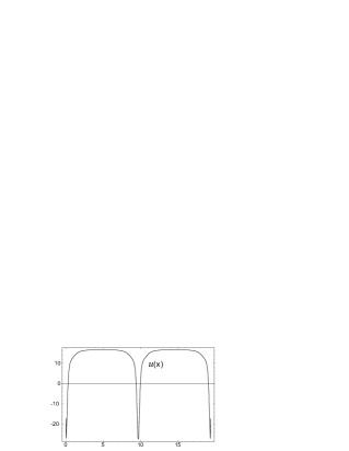
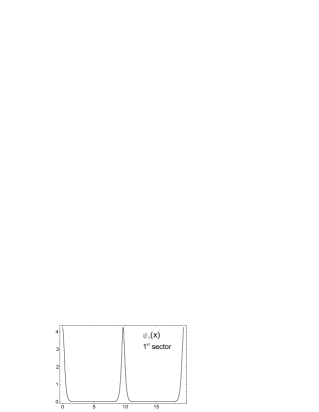
Periodic potential $u(x)$ for $m=0.999$.	$E_{0}=-20.41235597893$
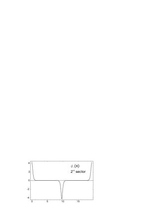
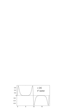
$E_{1}=-20.41235597887$	$E_{2}=0.577140437402$
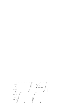
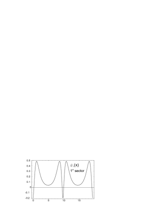
$E_{3}=0.577142188310$	$E_{4}=3.57339250870$
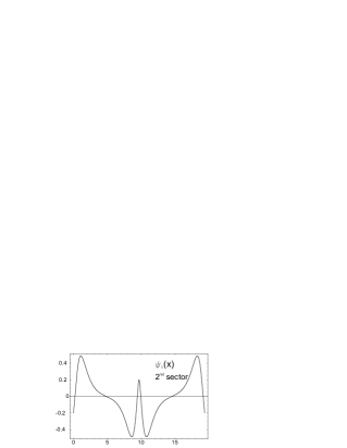
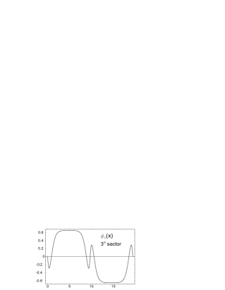
$E_{5}=3.57789250857$	$E_{6}=4.57514431434$

Figure 2. The periodic potential $u(x)$ in (112) for $\ell=4$ and $m=0.999$ has four gaps in its band spectrum. The seven algebraic eigenfunctions that correspond to the band edges are plotted together with their energies and the algebraic sector to which they belong.

7. Summary and Outlook

In this paper we introduced the notion of an exceptional polynomial subspace of $\mathcal{P}_{n}$ and identified those subspaces as the only ones that can give rise to new quasi-exactly solvable potentials in one dimension. For exceptional subspaces of co-dimension one ($\mathrm{X}_{1}$ subspaces), we claimed (Theorem 4.1) that $\mathcal{E}_{n}$ is the only $\mathrm{X}_{1}$ subspace up to an $\mathrm{SL}_{2}$ transformation. Next, we used the equivalence between an arbitrary second order differential operator and a Schrödinger operator to construct, characterize and classify $\mathrm{X}_{1}$ potentials, which are not Lie-algebraic. The characterization is done at the level of the potential invariant, and it involves an additional quadratic condition on the residues $k_{i}$ of the quotient $q(z)/p(z)$ of the coefficients of the second order operator. As in the Lie-algebraic case, the leading order component $p(z)$ of an $\mathrm{X}_{1}$ operator is a quartic and we have used $\mathrm{SL}_{2}$ covariance to classify them into canonical forms, leading to new quasi-exactly solvable families of elliptic, hyperbolic, trigonometric and rational potentials on the line. The new characterization of the QES condition at the level of parameters $k_{i}$ in the potential invariant allows to analyze the potentials that admit multiple algebraic sectors, corresponding to a residual symmetry in the choice of $k_{i}$ such that the potential remains unchanged. We have provided a classification of all such cases.

Future work involves extending this classification into two possible directions:

1. Exceptional subspaces of codimension two or higher. Some examples of $\mathrm{X}_{2}$ subspaces are known to exist, but a full classification is not yet available. The equivalence problem is considerably harder than in the $\mathrm{X}_{1}$ case.

2. Exceptional subspaces of polynomials in two or more variables. A full classification of exceptional Schrödinger in more than one variable operators seems unfeasible due to the lack of a constructive solution to the equivalence problem. Nevertheless, some examples of many-body quasi-exactly solvable models are known [2, 3], and we do not exclude that new many-body problems exist with invariant spaces of exceptional type.

References

• [1] Y. Brihaye and B. Hartmann. Quasi-exactly solvable (QES) equations with multiple algebraisations. Czechoslovak J. Phys., 53(11):993–998, 2003. Quantum groups and integrable systems.
• [2] L. Brink, A. Turbiner, and N. Wyllard. Hidden algebras of the (super) Calogero and Sutherland models. J. Math. Phys., 39(3):1285–1315, 1998.
• [3] F. Finkel, D. Gómez-Ullate, A. González-López, M. A. Rodríguez, and R. Zhdanov. $A_{N}$-type Dunkl operators and new spin Calogero-Sutherland models. Comm. Math. Phys., 221(3):477–497, 2001.
• [4] F. Finkel, A. González-López, and M. A. Rodríguez. A new algebraization of the Lamé equation. J. Phys. A, 33(8):1519–1542, 2000.
• [5] F. Gesztesy and R. Weikard. Elliptic algebro-geometric solutions of the KdV and AKNS hierarchies—an analytic approach. Bull. Amer. Math. Soc. (N.S.), 35(4):271–317, 1998.
• [6] D. Gómez-Ullate, N. Kamran, and R. Milson. Quasi-exact solvability beyond the sl(2) algebraization. arXiv:nlin.SI/0601053.
• [7] D. Gómez-Ullate, N. Kamran, and R. Milson. Structure theorems for linear and non-linear differential operators admitting invariant polynomial subspaces. arXiv:nlin.SI/0604070.
• [8] D. Gómez-Ullate, N. Kamran, and R. Milson. The Darboux transformation and algebraic deformations of shape-invariant potentials. J. Phys. A, 37(5):1789–1804, 2004.
• [9] D. Gómez-Ullate, N. Kamran, and R. Milson. Quasi-exact solvability and the direct approach to invariant subspaces. J. Phys. A, 38(9):2005–2019, 2005.
• [10] A. González-López, N. Kamran, and P. J. Olver. Normalizability of one-dimensional quasi-exactly solvable Schrödinger operators. Comm. Math. Phys., 153(1):117–146, 1993.
• [11] A. González-López and T. Tanaka. A new family of $N$-fold supersymmetry: type B. Phys. Lett. B, 586(1-2):117–124, 2004.
• [12] A. González-López and T. Tanaka. A novel multi-parameter family of quantum systems with partially broken $N$-fold supersymmetry. J. Phys. A, 38(23):5133–5157, 2005.
• [13] A. Khare and U. Sukhatme. Complex periodic potentials with a finite number of band gaps. J. Math. Phys., 47(6):062103, 22, 2006.
• [14] R. Milson. On the construction of quasi-exactly solvable Schrödinger operators on homogeneous spaces. J. Math. Phys., 36(10):6004–6027, 1995.
• [15] P. J. Olver. Equivalence, invariants, and symmetry. Cambridge University Press, Cambridge, 1995.
• [16] G. Post and A. Turbiner. Classification of linear differential operators with an invariant subspace of monomials. Russian J. Math. Phys., 3(1):113–122, 1995.
• [17] A. O. Smirnov. Finite-gap solutions of the Fuchsian equations. Lett. Math. Phys., 76(2-3):297–316, 2006.
• [18] K. Takemura. The Heun equation and the Calogero-Moser-Sutherland system. III. The finite-gap property and the monodromy. J. Nonlinear Math. Phys., 11(1):21–46, 2004.
• [19] A. Treibich and J.-L. Verdier. Revêtements tangentiels et sommes de $4$ nombres triangulaires. C. R. Acad. Sci. Paris Sér. I Math., 311(1):51–54, 1990.
• [20] A. Treibich and J.-L. Verdier. Au-delà des potentiels et revêtements tangentiels hyperelliptiques exceptionnels. C. R. Acad. Sci. Paris Sér. I Math., 325(10):1101–1106, 1997.
• [21] A. V. Turbiner. Quasi-exactly-solvable problems and ${\rm sl}(2)$ algebra. Comm. Math. Phys., 118(3):467–474, 1988.
• [22] A. G. Ushveridze. Quasi-exactly solvable models in quantum mechanics. Institute of Physics Publishing, Bristol, 1994.