Periodic-Orbit Theory of Level Correlations

Abstract

We present a semiclassical explanation of the so-called Bohigas-Giannoni-Schmit conjecture which asserts universality of spectral fluctuations in chaotic dynamics. We work with a generating function whose semiclassical limit is determined by quadruplets of sets of periodic orbits. The asymptotic expansions of both the non-oscillatory and the oscillatory part of the universal spectral correlator are obtained. Borel summation of the series reproduces the exact correlator of random-matrix theory.

Quantum spectra of individual chaotic systems can be phenomenologically described in terms of random-matrix theory (RMT) Stoeckmann ; Haake . This universality – asserted by the celebrated  Bohigas-Giannoni-Schmit conjecture (BGS) BGS – is an empirical fact, supported by a huge body of experimental and numerical data. Proving its conceptual origin remains one of the fundamental challenges in quantum or wave chaos.

Spectral fluctuations are conveniently characterized in terms of the two-point correlation function, $R(\epsilon)=\Delta^{2}\left\langle\rho(E+\frac{\epsilon\Delta}{2\pi})\rho(E-\frac{\epsilon\Delta}{2\pi})\right\rangle-1$, where $\rho(E)$ is the energy-dependent density of states, $\Delta\equiv 1/\langle\rho\rangle$ the mean level spacing and $\langle\cdot\rangle$ denotes averaging over the energy $E$. Predictions made by RMT for the two-point correlation function are fully universal in that they depend only on the parameter $\epsilon$, and the fundamental symmetries of the system under consideration. Specifically, the complex representation $R(\epsilon)=\lim_{\gamma\to 0}\text{Re}\;C(\epsilon^{+})$ where $\epsilon^{\pm}=\epsilon\pm i\gamma$ and $C(\epsilon^{+})=\frac{\Delta^{2}}{2\pi^{2}}\langle\mathrm{tr}\,G^{+}(E+\epsilon\Delta/2\pi)\,\mathrm{tr}\,G^{-}(E-\epsilon\Delta/2\pi)\rangle-\frac{1}{2}$ is employed, with $G^{\pm}(E)=(E\pm i\gamma\Delta/2\pi-H)^{-1}$ and $H$ the Hamiltonian. The Wigner–Dyson unitary and orthogonal symmetry classes (the only ones to be considered here) of RMT afford the asymptotic series

$$C(\epsilon^{+})\sim\begin{cases}\frac{1}{2(i\epsilon^{+})^{2}}-\frac{\mathrm{e}^{2i\epsilon^{+}}}{2(i\epsilon^{+})^{2}}&\mbox{unitary}\\ \frac{1}{(i\epsilon^{+})^{2}}+\sum_{n=3}^{\infty}\frac{(n-3)!(n-1)}{2(i\epsilon^{+})^{n}}&\\ +\,\mathrm{e}^{2i\epsilon^{+}}\sum_{n=4}^{\infty}\frac{(n-3)!(n-3)}{2(i\epsilon^{+})^{n}}&\text{orthogonal}\;.\end{cases}$$ (1)

In either case, $C(\epsilon^{+})$ is a sum of a non-oscillatory part (power series in $1/\epsilon^{+}$) and an oscillatory one ($\mathrm{e}^{2i\epsilon^{+}}$ times a series in $1/\epsilon^{+}$). Resumming the series by Borel summation techniques and extrapolating to small positive values of $\epsilon$, one obtains $R(\epsilon)+1\propto\epsilon^{\beta}$ for $\epsilon\to 0$, a signature of the level repulsion symptomatic for chaos ($\beta=1,2$ for the case of orthogonal, unitary symmetry, resp.)

The question to be addressed below is how to obtain the RMT prediction (1) for a concrete chaotic (globally hyperbolic) quantum system. A step in this direction was recently made EssenFF on the basis of Gutzwiller’s semiclassical periodic-orbit theory Gutzwiller . Gutzwiller represents the level density $\rho(E)$ as a sum over periodic orbits, whereupon the function $R(\epsilon)$ becomes a sum over orbit pairs Berry ; Argaman ; SR . Relevant contributions to that double sum were shown EssenFF to originate from orbit pairs which are identical, mutually time-reversed, or differ only by connections in certain close self-encounters. By summing over all distinct families of orbit pairs, the Fourier transform of $R(\epsilon)$, the spectral form factor $K(\tau)$, was found to coincide with the RMT prediction for times $t=\tau T_{H}$ smaller than the Heisenberg time $T_{H}=2\pi\hbar/\Delta$, the time needed to resolve the mean level spacing. The behavior of $K(\tau)$ for $\tau>1$, also known from RMT, was left unexplained.

We now want to fill the gap left. As results we will obtain the full expression for the correlation function in the case of unitary symmetry, and an asymptotic $1/\epsilon$-expansion amenable to Borel summation in the orthogonal case. The oscillatory term, Fourier transformed, then complements $K(\tau)$ to its full form at $\tau>1$. In many respects, our reasoning is inspired by the field theoretical formulation of RMT correlation functions AIE , notably the existence of “anomalous saddle points” in the nonlinear $\sigma$-model Kamenev . It also affords a new interpretation of ideas underlying the “bootstrapping” Bootstrap .

The basic idea of our approach is to consider representations of $C(\epsilon^{+})$ different from the standard one in terms of the product of a single retarded and advanced Green function. We start from the generating function

$$Z=\left\langle\frac{\det(E_{C}^{+}-H)\det(E_{D}^{-}-H)}{\det(E_{A}^{+}-H)\det(E_{B}^{-}-H)}\right\rangle\,$$ (2)

where $E_{A,B,C,D}^{\pm}$ are energies in the vicinity of $E$ defined by $E_{A,B,C,D}^{\pm}=E+\epsilon_{A,B,C,D}^{\pm}\Delta/2\pi$. From $Z$, the complex correlator can be accessed as

$$\lim_{\gamma\to 0}C(\epsilon^{+})=-\frac{1}{2}+2\frac{\partial^{2}Z}{\partial\epsilon_{A}^{+}\partial\epsilon_{B}^{-}}\big{|}_{\|,\times}\;.$$ (3)

The two derivatives produce the product $({\rm tr}G^{+})({\rm tr}G^{-})$ under the energy average. If we subsequently identify the energies “columnwise” ($\|$): $\epsilon_{A}^{+}=\epsilon_{C}^{+}={\epsilon^{+}}$, $\epsilon_{B}^{-}=\epsilon_{D}^{-}=-{\epsilon^{+}}$, or “crosswise”($\times$): $\epsilon_{A}^{+}={\epsilon^{+}}$, $\epsilon_{B}^{-}=-{\epsilon^{+}}$, $\epsilon_{C}^{+}=-{\epsilon^{-}}$, $\epsilon_{D}^{-}={\epsilon^{-}}$, $\gamma\to 0$ the ratio of determinants approaches unity. The first representation for $C(\epsilon^{+})$ does not even require the limit $\gamma\to 0$; it is widely used in RMT. The second representation is crucial for us. Importantly, the semiclassical approximation of either of these two exact representations misses contributions to $Z$, and therefore to $C(\epsilon^{+})$: the first representation yields only the non-oscillatory contributions, and the second (without ”$-\frac{1}{2}$”) only the oscillatory ones; adding both we will recover the universal two-point correlator.

To see the emergence of these structures, let us represent the determinants in (2) as

$$\det\,(E_{A}^{+}-H)^{-1}=\exp\Big{\{}-\int^{E_{A}^{+}}dE\,\mathrm{tr}\,G^{+}(E)\Big{\}}$$ (4)

$$\sim \mathrm{const}\times\exp\Big{(}i\pi E_{A}^{+}/\Delta+\sum_{a}F_{a}\mathrm{e}^{\frac{i}{\hbar}S_{a}(E_{A}^{+})}\Big{)}\,,$$

where the last line invokes the semiclassical expansion of the integrated Green function into a smooth (Weyl) average and a fluctuating (Gutzwiller) part; the latter is a sum of periodic orbits $a$ with action $S_{a}$ and stability amplitude $F_{a}$; for simplicity, we assume the average level density $1/\Delta$ to be constant; the periodic-orbit sum converges for $\mathrm{Im}E_{A}^{+}$ large enough; the “const” in (4) comes from the lower limit of the energy integral and cancels from the ratio of determinants in $Z$.

Expanding the exponential in (4) we get a sum over non-ordered sets of orbits $A$ (“pseudo-orbits”),

$$\det(E_{A}^{+}-H)^{-1}\!\!\sim\!\mathrm{const}\times\mathrm{e}^{i\pi E_{A}^{+}/\Delta}\sum_{A}\!F_{A}\mathrm{e}^{\frac{i}{\hbar}S_{A}(E_{A}^{+})}\,.$$ (5)

A pseudo-orbit $A$ may involve any number $n_{A}$ of component orbits ($n_{A}=0$ pertains to the empty set which contributes unity to the sum); $F_{A}$ is the product of the stability amplitudes and $S_{A}$ the cumulative action of all component orbits. Expressing all four determinants in (2) similarly to (4,5) (e. g., using $\det(E_{B}^{-}-H)=(\det(E_{B}^{+}-H))^{\ast}$) and writing $S(E+\epsilon\Delta/2\pi)\sim S(E)+T(E)\epsilon\Delta/2\pi\;$ ($T$ is the period of an orbit, or the sum of periods in a pseudo-orbit) we approximate the generating function as

$$Z\;\sim\!\!\!\! \mathrm{e}^{\frac{i}{2}(\epsilon_{A}^{+}-\epsilon_{B}^{-}-\epsilon_{C}^{+}+\epsilon_{D}^{-})}$$

$$\times\big{\langle}\textstyle{\exp\big{(}\sum_{a}F_{a}\mathrm{e}^{\frac{i}{\hbar}S_{a}(E)+i\frac{T_{a}}{T_{H}}\epsilon_{A}^{+}}+\sum_{b}F_{b}^{\ast}\mathrm{e}^{-\frac{i}{\hbar}S_{b}(E)-i\frac{T_{b}}{T_{H}}\epsilon_{B}^{-}}}$$

$$\!\!-\textstyle{\sum_{c}F_{c}\,\mathrm{e}^{\frac{i}{\hbar}S_{c}(E)+i\frac{T_{c}}{T_{H}}\epsilon_{C}^{+}}-\sum_{d}F_{d}^{\ast}\mathrm{e}^{-\frac{i}{\hbar}S_{d}(E)-i\frac{T_{d}}{T_{H}}\epsilon_{D}^{-}}\big{)}\big{\rangle}}$$

$$= \mathrm{e}^{\frac{i}{2}(\epsilon_{A}^{+}-\epsilon_{B}^{-}-\epsilon_{C}^{+}+\epsilon_{D}^{-})}\big{\langle}\!\!\sum_{A,B,C,D}\!\!F_{A}F_{B}^{\ast}F_{C}F_{D}^{\ast}(-1)^{n_{C}+n_{D}}$$

$$\hskip 56.9055pt\times\;\mathrm{e}^{i(S_{A}(E)-S_{B}(E)+S_{C}(E)-S_{D}(E))/\hbar}$$

$$\hskip 56.9055pt\times\;\mathrm{e}^{i(T_{A}\epsilon_{A}^{+}-T_{B}\epsilon_{B}^{-}+T_{C}\epsilon_{C}^{+}-T_{D}\epsilon_{D}^{-})/T_{H}}\big{\rangle}\;.$$

Here, the mean density produces a phase factor $\mathrm{\ e}^{\frac{i}{2}(\epsilon_{A}^{+}-\epsilon_{B}^{-}-\epsilon_{C}^{+}+\epsilon_{D}^{-})}$. When representing the correlator as in (3), that phase factor turns into 1 and $\mathrm{e}^{2i\epsilon}$ for the columnwise and crosswise identifications of energies, respectively. Indeed, then, we can recover either the non-oscillatory or the oscillatory contributions to $C(\epsilon^{+})$.

Another phase factor involves the difference $\Delta S\equiv S_{A}(E)-S_{B}(E)+S_{C}(E)-S_{D}(E)$ between the cumulative actions of $(A,C)$ and $(B,D)$. Due to this factor, systematic contributions in the limit $\hbar\to 0$ can arise only for quadruplets of pseudo-orbits whose action difference is of the order of $\hbar$ or smaller.

The most basic of quadruplets have each of the component orbits of $A$ and $C$ repeated in either $B$ or $D$, such that $\Delta S=0$. These “diagonal quadruplets” may be summed by a lowest-order cumulant expansion: denoting the periodic-orbit sums in the exponent of (Periodic-Orbit Theory of Level Correlations) by $X$, we may write $\left\langle\mathrm{e}^{X}\right\rangle_{\rm diag}=\exp\{\left\langle X^{2}\right\rangle_{\rm diag}/2\}$, wherein $\left\langle X^{2}\right\rangle_{\rm diag}$ contains only pairs of identical orbits. We obtain

$$Z_{\mathrm{diag}}\sim \exp\textstyle{{\left\langle X^{2}\right\rangle_{\mathrm{diag}}/2}}$$ (8)

$$\sim \textstyle{\exp\big{\langle}\sum_{a}|F_{a}|^{2}\big{(}\mathrm{e}^{i\frac{T_{a}}{T_{H}}(\epsilon_{A}^{+}-\epsilon_{B}^{-})}-\mathrm{e}^{i\frac{T_{a}}{T_{H}}(\epsilon_{A}^{+}-\epsilon_{D}^{-})}}\big{)}$$

$$\hskip 17.07182pt\textstyle{-\sum_{c}|F_{c}|^{2}\big{(}\mathrm{e}^{i\frac{T_{c}}{T_{H}}(\epsilon_{C}^{+}-\epsilon_{B}^{-})}-\mathrm{e}^{i\frac{T_{c}}{T_{H}}(\epsilon_{C}^{+}-\epsilon_{D}^{-})}\big{)}\big{\rangle}}.$$

Relying on ergodicity, the resulting sums over orbits may be evaluated by the sum rule of Hannay and Ozoria de Almeida HOdA , $\sum_{a}|F_{a}|^{2}(\cdot)\approx\int_{T_{0}}^{\infty}\frac{dT}{T}(\cdot)$; the lower limit of the integration is a minimal period $T_{0}$ starting from which periodic orbits behave approximately ergodically. By this rule, e.g., the first sum turns into $-\ln(i(\epsilon_{A}^{+}-\epsilon_{B}^{-}))+\mathrm{const}+\mathcal{\ O}(\hbar)$. All four sums yield

$$Z_{\mathrm{diag}}\sim\mathrm{e}^{\frac{i}{2}(\epsilon_{A}^{+}-\epsilon_{B}^{-}-\epsilon_{C}^{+}+\epsilon_{D}^{-})}\left(\frac{(\epsilon_{A}^{+}-\epsilon_{D}^{-})(\epsilon_{C}^{+}-\epsilon_{B}^{-})}{(\epsilon_{A}^{+}-\epsilon_{B}^{-})(\epsilon_{C}^{+}-\epsilon_{D}^{-})}\right)^{\kappa},$$ (9)

with $\kappa=1$ for the unitary class. For the orthogonal class we must also consider pairs of mutually time reversed orbits. Therefore, each sum in (8) must be multiplied by 2 whereupon in the final result (9) we have $\kappa=2$.

Taking derivatives and columnwise identified energies, we recover the leading non-oscillatory contribution to the two-point correlator, $(i\epsilon^{+})^{-2}/\beta$. Crosswise identified energies yield the oscillatory contribution $-\mathrm{\ e}^{2i\epsilon}(i\epsilon)^{-2}/2$ for $\beta=2$ (thus completely reproducing (1)), while for $\beta=1$ we get zero, i. e., no oscillatory term arises up to $\mathcal{O}(\epsilon^{-2})$, again as in RMT.

Going beyond the above level of approximation, we note that small phases may also arise from component orbits $B$ and $D$ differing from $A$ and $C$ in topology, but only weakly in action. By way of example, consider a pseudo-orbit $A$ with just one component, while $C$ is the empty set. Assume that $A$ contains a so-called “2-encounter”, where two stretches of the orbit come close in phase space. This situation is depicted in Fig. 1a (where the phase-space encounter contains a crossing in configuration space). The two stretches start and end at altogether four “ports”, and are connected to each other through two external “links”foot . Changing the way the ports are connected inside the encounter, as illustrated by the dashed line in Fig. 1a, we obtain two disjoint periodic orbits, each containing one link and one encounter stretch. The existence proof of the latter two orbits as exponentially close to the links of the original orbit requires chaos and was in essence given in Ref. SR . These two orbits can either both be included in $B$ such that $D$ remains empty, or vice versa, or one is included in $B$ and the other one in $D$. At any rate the cumulative actions of $(A,C)$ and $(B,D)$ almost coincide.

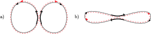
Figure 1: “Diagrams” of simplest (pseudo-)orbits in configuration space. Arrows indicate sense of traversal.

A second example, a so-called Sieber/Richter pair SR , is shown in Fig. 1b: Here two orbits differ in an encounter wherein two stretches are approximately mutually time-reversed. One of these orbits is included in $A$ leaving $C$ empty or vice versa, whereas the other is included in $B$ or $D$. Such orbit pairs exist only in time-reversal invariant systems since we assume that the sense of motion on an encounter stretch or a link can be reverted in time.

More complicated quadruplets involve any number of orbits, and $(A,C)$ and $(B,D)$ can differ in any number of encounters where arbitrarily many stretches come close in phase space (modulo time reversal for time-reversal invariant systems); encounters may be self-encounters within periodic-orbit components in a pseudo-orbit, mutual encounters of different periodic orbits within one pseudo-orbit, or even from different pseudo-orbits.

As in the diagonal approximation some of the component orbits of $(A,C)$ may just be repeated in $(B,D)$. To evaluate the generating function, we must sum over all quadruplets of this type. We can split the sum into one over the “diagonal” parts of these quadruplets and one over the orbits differing in encounters. The first subsum yields $Z_{\mathrm{diag}}$ as in (9) such that $Z=Z_{\mathrm{diag}}(1+Z_{\mathrm{off}})$ with

$$Z_{\mathrm{off}}=\sum_{A,B,C,D\atop{\text{diff. in enc.}}} \Big{\langle}F_{A}F_{B}^{*}F_{C}F_{D}^{*}(-1)^{n_{C}+n_{D}}$$

$$\times\,\mathrm{e}^{i\Delta S/\hbar}\mathrm{e}^{i(T_{A}\epsilon_{A}^{+}-T_{B}\epsilon_{B}^{-}+T_{C}\epsilon_{C}^{+}-T_{D}\epsilon_{D}^{-})/T_{H}}\Big{\rangle}\,.$$

To find $Z_{\mathrm{off}}$ we must classify and count quadruplets with encounters. Their topological “structure” must be dealt with first. To that end we number all encounter stretches (stretches, for short) of $A$ and $C$. Starting with an arbitrary stretch in the orbit with the smallest number of stretches, we number the stretches in that orbit in their order of traversal; we continue with the orbit with the second-smallest number of stretches, etc. Each structure now corresponds to one way of (i) grouping these numbered stretches into encounters, (ii) choosing their mutual orientation if the system is time-reversal invariant, (iii) changing connections inside the encounters, and (iv) dividing the original orbits among $A$ and $C$ and the reconnected orbits among $B$ and $D$. Quadruplets of pseudo-orbits can typically be described by several equivalent structures: If we denote by $\omega_{\mu}$ the number of component orbits of $A,C$ with $\mu$ encounter stretches, there are $\prod_{\mu}\mu^{\omega_{\mu}}\omega_{\mu}!$ ways of choosing first stretches, and ordering the $\omega_{\mu}$ orbits with fixed $\mu$. When summing over structures, we must divide out that overcounting factor.

Next, pseudo-orbit quadruplets are characterized by phase-space separations between the encounter stretches. To measure separations for an $l$-encounter, we introduce a Poincaré surface of section orthogonal to the original orbit in an arbitrary reference point in one of the stretches. The other stretches pierce through the same section in $(l-1)$ further points; their phase-space separation from the first piercing can be decomposed into components $u_{i}$ and $s_{i}$ along the unstable and stable manifolds. As shown in Ref.EssenFF , the encounter contributes to the action difference as $\Delta S=\sum_{j}s_{j}u_{j}$ and has a duration $t_{\mathrm{enc}}=\frac{1}{\lambda}\ln\frac{c^{2}}{\max_{j}|s_{j}|\times\max_{k}|u_{k}|}$ where $\lambda$ is the Lyapunov exponent and $c$ a constant whose value is unimportant.

The sum over $A,B,C,D$ in (Periodic-Orbit Theory of Level Correlations) can be written as a sum over structures and an integral over $s,u$ and the link durations $t$. The measure to be used EssenFF ; Transport obtains a factor $1/\Omega^{l-1}t_{\mathrm{enc}}$ from each $l$-encounter, with $\Omega$ the volume of the energy shell. The factor $1/\Omega^{l-1}$ arises from ergodicity and gives the uniform probability density for the $l-1$ later piercings to have given stable and unstable differences from the reference one; the factor $1/t_{\mathrm{enc}}$ compensates an overcounting due to the fact that the Poincaré section may be placed anywhere inside the encounter.

We next split the phase-space integral into factors representing the links and the encounters. To do so, we write the time $T_{A}$ as a sum of durations of all links and encounter stretches which belong to $A$ before reconnection; $T_{B}$, $T_{C}$, and $T_{D}$ are decomposed similarly. We then obtain an integral $\int_{0}^{\infty}dt\;\mathrm{e}^{it(\epsilon_{\text{$A$ or $C$}}^{+}-\epsilon_{\text{$B$ or $D$}}^{-})/T_{H}}$ for each link (belonging to $A$ or $C$ before reconnection and to $B$ or $D$ afterwards) and an integral $\int\!d^{l-1}\!sd^{l-1}\!u\frac{1}{\Omega^{l-1}t_{\mathrm{enc}}}\!\mathrm{\ e}^{\frac{i}{\hbar}\sum_{j}\!s_{j}u_{j}}\mathrm{e}^{i(l_{A}\epsilon_{A}^{+}-l_{B}\epsilon_{B}^{-}+l_{C}\epsilon_{C}^{+}-l_{D}\epsilon_{D}^{-})\frac{t_{\mathrm{enc}}}{T_{H}}}$ for each encounter (with $l_{A},l_{B},l_{C},l_{D}$ the numbers of stretches of the encounter belonging to $A,B,C,D$, and $l_{A}+l_{C}=l_{B}+l_{D}$.) Evaluating these integrals as in Transport we obtain a factor $i(\epsilon_{\text{$A$ or $C$}}^{+}-\epsilon_{\text{$B$ or $D$}}^{-})^{-1}$ for each link a factor $i(l_{A}\epsilon_{A}^{+}-l_{B}\epsilon_{B}^{-}+l_{C}\epsilon_{C}^{+}-l_{D}\epsilon_{D}^{-})$ for each encounter, while $T_{H}$ cancels out. In this way, $Z_{\mathrm{off}}$ becomes the sum over structures

$$Z_{\mathrm{off}}\!\sim\!\!\!\sum_{\mathrm{struct}}\textstyle{\!\!\frac{\kappa^{n_{B}+n_{D}}\prod_{\mathrm{enc}}i(l_{A}\epsilon_{A}^{+}-l_{B}\epsilon_{B}^{-}+l_{C}\epsilon_{C}^{+}+l_{D}\epsilon_{D}^{-})}{\!(-1)^{n_{C}+n_{D}}\!\prod_{\mu}\mu^{\omega_{\mu}}\omega_{\mu}!\!\prod_{\mathrm{links}}(-i)(\epsilon_{\text{$A$ \!or \!$C$}}^{+}\,-\,\epsilon_{\text{$B$ \!or \!$D$}}^{-})}},$$ (11)

where for $\beta=1$ the factor $\kappa^{n_{B}+n_{D}}$ accounts for the two different senses of motion on the “reconnected” orbits. Summarily referring to the linear combinations of the $\epsilon_{A,B,C,D}^{\pm}$ in the link and encounter factors as $\epsilon$, we infer that $Z_{\mathrm{off}}$ is a power series in $1/\epsilon$. The term $(1/\epsilon)^{m}$ is provided by all structures with $m=L-V$, with $V$ the number of encounters and $L$ the number of stretches in a structure; note $L>V$. This remark allows to draw all “diagrams” contributing to each of the first few orders of the expansion and to evaluate their contributions.

For instance, the order $m=1$ is determined by the two diagrams in Fig. 1, whereas for $m=2$ we need quadruplets with two 2-encounters or one 3-encounter. In the unitary case, all these quadruplets either yield vanishing contributions to $Z$ (after summing over all possible assignments of orbits to $A,B,C,D$) or mutually cancel. Reassuringly, the low-order analysis of the general expression above complies with the fact that for $\beta=2$ the diagonal approximation exhausts the RMT result.

In the orthogonal case, off-diagonal contributions remain and the non-oscillatory and the oscillatory parts of the correlator $C(\epsilon)$ are obtained according to (3). Not surprisingly, the non-oscillatory terms are determined only by  pairs of orbits (such as Fig. 1b) known from the previous work on the small-time form factor; in the present language, either $A$ or $C$, and either $B$ or $D$ are empty. All genuine pseudo-orbits end up contributing nothing. The first oscillatory term, $\propto\mathrm{e}^{2i\epsilon}/\epsilon^{4}$, does involve non-trivial pseudo-orbit quadruplets. It can be attributed to quadruplets of orbits involving two Sieber/Richter pairs; further (mutually canceling) diagrams are archived in an appendix. Proceeding to all orders we get the full asymptotic expansions (1) à la RMT.

The form factor is finally obtained from the complex correlator as $K(\tau)=\frac{1}{2\pi}\int_{-\infty+ia}^{\infty+ia}\mathrm{\ e}^{-i2\epsilon\tau}C(\epsilon)d\epsilon,\quad a>0$. Substitution of our expansion (1) for $C(\epsilon)$ and term-by-term integration produces, for both symmetry classes, two analytic functions different from zero for $\mathrm{Re}\,\tau>0$ and $\mathrm{Re}\,\tau>1$, respectively, which sum up to the RMT form factor. The Laplace transform of the result reproduces the exact complex correlator of RMT as $C(\epsilon)=2\int_{0}^{\infty}\mathrm{\ e}^{i2\tau\epsilon}K(\tau)d\tau$ including the power law of its real part for $\epsilon\to 0$, i.e., level repulsion. For conditions under which such a back-and-forth Laplace transformation (Borel summation) uniquely restores a function from its asymptotic series see Sokal .

We conclude with the following remarks. Implicit to our present analysis is a specific order of two limits. These are the semiclassical limit which brings in the periodic-orbit sum à la Gutzwiller in (4), alluded to as $\lim_{\Delta\to 0}$ below, and the vanishing of the imaginary part ${\rm Im}E^{+}=\gamma\Delta/2\pi$ of the complex energies and of ${\rm Im}\epsilon^{+}=\gamma$, i. e. $\lim_{\gamma\to 0}$. We need the condition $\gamma\Delta/\Delta=\gamma>1$ to make the periodic-orbit contributions to our asymptotic expansions well defined. It is worth noting that this condition effectively limits the orbit periods as $T<T_{H}$; see Eq. (Periodic-Orbit Theory of Level Correlations) where the final exponential includes a damping ${\rm e}^{-\gamma(T_{A}+T_{B}+T_{C}+T_{D})/T_{H}}$. In our limit sequence (first $\Delta\to 0$ with $\gamma>1$ fixed, then $\gamma\to 0$) the two representations, $\times$ and $\parallel$, become inequivalent, and resolve different parts of the two-point function (oscillatory and non-oscillatory); separate asymptotic expansions for both are required to recover the full information. This complementarity phenomenon is reflected in the structure of the field theoretical approach to spectral statistics as well: the functional integral representation of $Z$ in RMT is controlled by two saddle points Kamenev . In the limit $\gamma\ll 1$, both saddles equally contribute and give $C$ in full in either representation, $\parallel$ and $\times$; one saddle provides the non–oscillatory part of $C$, the other the oscillatory part. However, for $\gamma>1$, the oscillatory part gets exponentially suppressed as ${\rm e}^{-\gamma}$ in the $\parallel$-representation, while the $\times$-representation has the non-oscillatory part exponentially damped. The perturbative $\epsilon^{-1}$–expansions of the surviving parts, on the other hand, quantitatively agree with the results of our semiclassical analysis, to all orders in $1/\epsilon$. We shall further discuss analogies semiclassics/field theory in a forthcoming paper.

We thank the SFB/TR12 of the Deutsche Forschungsgemeinschaft and the EPSRC for funding and Ben Simons and Hans-Jürgen Sommers for fruitful discussions.

Appendix: Leading contributions

To illustrate our results, we evaluate the contributions of the simplest quadruplets of pseudo-orbits. We start with the ”diagram” in Fig. 1a, where an orbit involving an encounter of two almost parallel stretches decomposes into two disjoint partner orbits. First, assume that the initial orbit is included in the pseudo-orbit $A$. Each of the two partner orbits can be included either in $B$ or in $D$. This leads to four different possibilities, whose contributions to $Z_{\rm off}$ can be evaluated using the diagrammatic rules introduced above,

$$\frac{2i\epsilon_{A}^{+}-2i\epsilon_{B}^{-}}{(-i(\epsilon_{A}^{+}-\epsilon_{B}^{-}))^{2}}-2\frac{2i\epsilon_{A}^{+}-i\epsilon_{B}^{-}-i\epsilon_{D}^{-}}{(-i(\epsilon_{A}^{+}-\epsilon_{B}^{-}))(-i(\epsilon_{A}^{+}-\epsilon_{D}^{-}))}$$ (12)

$$+\frac{2i\epsilon_{A}^{+}-2i\epsilon_{D}^{-}}{(-i(\epsilon_{A}^{+}-\epsilon_{D}^{-}))^{2}}=0\,.$$

In a similar way, all possibilities with the initial orbits included in $B,C$ or $D$ also sum to zero. The orbit quadruplets corresponding to the ”diagram” in Fig. 1a thus yields no net contribution.

Next, we consider Sieber/Richter pairs as in Fig. 1b. These pairs require time-reversal invariance and therefore exist only in the orthogonal case. According to our diagrammatic rules, Sieber/Richter pairs where, say, the original orbit is included in $A$ and its partner is included in $B$ yield a contribution $\frac{2}{i(\epsilon_{A}^{+}-\epsilon_{B}^{-})}$ to $Z_{\rm off}$. All other possibilities to assign the two orbits to $A,B,C,D$ can be treated in the same way. Summation thus yields $2F$, where

$$F\equiv\frac{1}{i(\epsilon_{A}^{+}-\epsilon_{B}^{-})}-\frac{1}{i(\epsilon_{A}^{+}-\epsilon_{D}^{-})}-\frac{1}{i(\epsilon_{C}^{+}-\epsilon_{B}^{-})}+\frac{1}{i(\epsilon_{C}^{+}-\epsilon_{D}^{-})}$$ (13)

Upon taking derivatives and identifying the energies in a columnwise way, Sieber/Richter pairs yield a non-oscillatory contribution $\frac{1}{(i\epsilon)^{3}}$ to the complex correlator, whereas the corresponding oscillatory term (obtained after crosswise identification of energies) vanishes.

The simplest quadruplets beyond Fig. 1a and b are those with $m=L-V=2$, i.e., either with two $2-$encounters or one $3-$encounter. These quadruplets are shown in Fig. 2, grouped into columns labeled by $1:1$, $1:2$, $1:3$, and $2:2$. Here the first number counts the orbits before reconnection (black lines) whereas the second number counts the orbits after reconnection (colored or gray lines). To evaluate the resulting contributions, we have to sum over all ways of distributing these orbits among $A$, $B$, $C$, and $D$ (placing the former orbits in $A$ or $C$ and the latter in $B$ or $D$ or vice versa) and apply the above diagrammatic rules.

We have done so, and obtained the following result: All quadruplets of pseudo-orbits that do not require time-reversal invariance (in the shaded rows) give mutually canceling contributions to $Z_{\rm off}$, and thus no off-diagonal contributions to the correlator.

For time-reversal invariant systems $Z_{\rm off}$ is non-zero. When taking derivatives and identifying energies in a columnwise way, we see that non-oscillatory terms in $C(\epsilon)$ arise only from quadruplets associated to $1:1$, summing up to $\frac{3}{2(i\epsilon)^{4}}$.

In contrast, non-vanishing oscillatory contributions (obtained through the crosswise representation) arise only from the quadruplets of type $2:2$. The first and third of these diagrams in Fig. 2 mutually cancel. The leading off-diagonal contribution to the oscillatory part can thus be attributed solely to the second diagram, composed of two Sieber/Richter pairs . For these quadruplets the sum over possible assignments to $A$, $B$, $C$, and $D$ can be performed independently for the two pairs. We are therefore left with the square of the contribution of a single Sieber/Richter pair, which must be divided by 2 since the divisor $\prod_{\lambda}\omega_{\lambda}!$ in (11) is now equal to 2. We thus obtain a term $2F^{2}$ in $Z_{\rm off}$ and a contribution

$$\frac{\partial^{2}(Z_{\rm diag}2F^{2})}{\partial\epsilon_{A}^{+}\partial\epsilon_{B}^{-}}{\Big{|}}_{\times}=\frac{e^{2i\epsilon}}{2\epsilon^{4}}$$ (14)

to $C(\epsilon)$, coinciding with the leading oscillatory term in the RMT prediction (1).

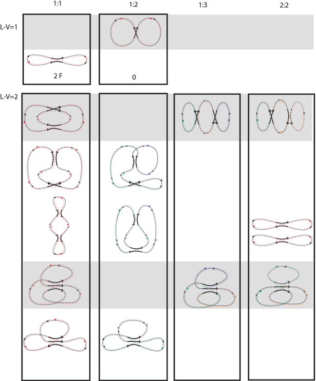
Figure 2: ”Diagrams” responsible for the asymptotic expansion of the complex correlator up to order ${\cal O}(\frac{1}{\epsilon^{4}})$. The shaded rows contain pairs which exist even in the absence of time-reversal invariance; the rest exists only in the orthogonal case. The quadruplets in the first column are marked by $1:1$ since they involve $one$ orbit before and after reconnection. In others columns, the number of orbits before and after reconnection is $1:2,1:3$ and $2:2$, respectively. Pseudo-orbits containing a 3-encounter can have several partners depending on the reconnection. The contributions to $Z_{\rm off}$ as defined in (11) are shown explicitly for pairs with $L=2$ links and $V=1$ encounter. For $m=L-V=2$, the resulting contributions to $Z_{\rm off}$ are rather involved and will be presented in a forthcoming publication.

References

- (1) H.-J. Stöckmann, Quantum Chaos: An Introduction (Cambridge University Press, Cambridge, England, 1999).
- (2) F. Haake, Quantum Signatures of Chaos, 2nd ed. (Springer, Berlin, 2001).
- (3) O. Bohigas, M. J. Giannoni, and C. Schmit, Phys. Rev. Lett. 52, 1 (1984); S. W. McDonald and A. N. Kaufman, Phys. Rev. Lett. 42, 1189 (1979); G. Casati, F. Valz-Gris, and I. Guarneri, Lett. Nuovo Cim. 28, 279 (1980); M. V. Berry, Ann. Phys. (N.Y.) 131, 163 (1981).
- (4) S. Müller, S. Heusler, P. Braun, F. Haake, and A. Altland, Phys. Rev. Lett. 93, 014103 (2004); Phys. Rev. E 72 , 046207 (2005).
- (5) M. Gutzwiller, Chaos in Classical and Quantum Mechanics (Springer, New York, 1990).
- (6) M. V. Berry, Proc. R. Soc. Lond., Ser. A 400, 229 (1985).
- (7) N. Argaman et. al., Phys. Rev. Lett. 71, 4326 (1993).
- (8) M. Sieber and K. Richter, Physica Scripta T90, 128 (2001); M. Sieber, J. Phys. A 35, L613 (2002).
- (9) A. Altland, S. Iida, and K.B. Efetov, J. Phys. A 26, 3545 (1993).
- (10) A. V. Andreev and B. L. Altshuler, Phys. Rev. Lett. 75, 902 (1995); A. Kamenev and M. Mézard, Phys. Rev. B60, 3944 (1999)
- (11) E. B. Bogomolny and J. P. Keating, Phys. Rev. Lett. 77, 1472 (1996).
- (12) J. H. Hannay and A. M. Ozorio de Almeida, J. Phys. A 17, 3429 (1984).
- (13) In EssenFF ; SR ; Transport , the term “loop” was used instead of “link”; link is more appropriate for the majority of diagrams since most links start and end at different encounters.
- (14) S. Heusler, S. Müller, P. Braun, and F. Haake, Phys. Rev. Lett 96, 066804 (2006); P. Braun, S. Heusler, S. Müller, and F. Haake, J. Phys. A 39, L159 (2006).
- (15) A.D. Sokal, J. Math. Phys. 21, 261 (1980).