theDOIsuffix \VolumeXX \Issue1 \Month01 \Year2003 \pagespan1 \Receiveddate \Reviseddate \Accepteddate \Dateposted
Vibration of Generalized Double Well Oscillators
Abstract
We have applied the Melnikov criterion to examine a global homoclinic bifurcation and transition to chaos in a case of a double well dynamical system with a nonlinear fractional damping term and external excitation. The usual double well Duffing potential having a negative square term and positive quartic term has been generalized to a double well potential with a negative square term and a positive one with an arbitrary real exponent . We have also used a fractional damping term with an arbitrary power applied to velocity which enables one to cover a wide range of realistic damping factors: from dry friction to turbulent resistance phenomena . Using perturbation methods we have found a critical forcing amplitude above which the system may behave chaotically. Our results show that the vibrating system is less stable in transition to chaos for smaller satisfying an exponential scaling low. The critical amplitude as an exponential function of . The analytical results have been illustrated by numerical simulations using standard nonlinear tools such as Poincare maps and the maximal Lyapunov exponent. As usual for chosen system parameters we have identified a chaotic motion above the critical Melnikov amplitude .
keywords:
Duffing oscillator, Melnikov criterion, chaotic vibration1 Introduction
A nonlinear oscillator with single or double well potentials of the Duffing type and linear damping is one of the simplest systems leading to chaotic motion studied by [1, 2, 3, 4]. The problem of its nonlinear vibrations has attracted researchers from various fields of research across natural science and physics [4, 5, 6], mathematics [8] mechanical engineering [10, 11, 14, 12, 13]; and finally electrical engineering [1, 2, 3]. This system, for a negative linear part of stiffness, shows homoclinic orbits, and the transition to chaotic vibration can be treated analytically via the Melnikov method [7]. Such a treatment has been already performed successfully to selected problems with various potentials [8, 9, 14]. Vibrations of a single Duffing oscillator have got a large bibliography [1, 2, 3, 4, 5, 6, 8, 9, 10, 11, 12, 13, 14, 15, 16, 17, 18]. In the last decade coupled Duffing oscillators [19, 20, 21, 22, 23] with numerous modifications to potential and forcing parts have been studied. On the other hand the problem of nonlinear damping in chaotically vibrating system has not been discussed in detail. Some insight into this problem can also be found in the context of self excitation effects
[15, 19, 22, 23, 25, 24, 26]. and dry friction effects [33, 34, 35, 36] In the paper by Trueba et al. [16], the systematic discussion on square and cubic damping effects on global homoclinic bifurcations in the Duffing system has been given. Recently Trueba et al. [17] and Borowiec et al. [18] have analyzed a single degree of freedom nonlinear oscillator with the Duffing potential and fractional damping. Different aspects fractionally damped systems have been studied recently by Mickens et al., Gottlieb, and Mickens [27, 28, 29]. On the other hand Maia et al. and Padovan and Sawicki [30, 32, 31] analyzed similar systems where fractional damping have been introduced in different way through a fractional derivative. Awrejcewicz and Holicke [37] and more recently Awrejcewicz and Pyryev [38] applied Melnikov’s method in the presence of dry friction for a stick-slip oscillator. More general introduction to the problem of non-smooth or discontinuous mechanical systems can be found in [39, 40].
In the present paper we revisit this problem looking for a global homoclinic bifurcation and transition to chaotic vibrations in a system described by a more general double well potential where its usual positive quartic term has been generalized to term with an arbitrary real exponent grater than 2. Below we would also apply a nonlinear damping term with a fractional exponent covering the gap between viscous, dry friction and turbulent damping phenomena.
The equation of motion has the following form:
| (1) |
where is displacement and velocity, respectively, while the external force :
| (2) |
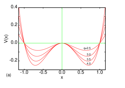
and corresponding potential (Fig. 1a) is defined as:
| (3) |
where is a real number. In spite of the definition (Eq. 3) in terms of absolute value it is still a function of class if only (see Appendix A).
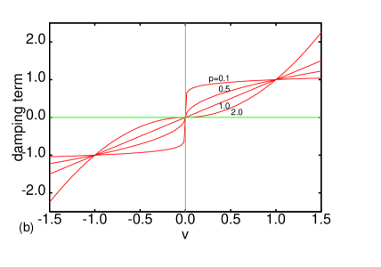
The non-linear damping term is defined by the exponent :
| (4) |
In Fig. 1b we have plotted the above function versus velocity () for few values of . Note that, the case (see in Fig. 1b for a relatively small velocity) mimics the dry friction phenomenon [33, 34].
2 Melnikov Analysis
We start our analysis with the unperturbed Hamiltonian:
| (5) |
Note that for our choice of potentials and (Fig. 1a) has the three nodal points (, 0, 1) where the middle one () corresponds to the local peak at the saddle point. The existence of this point with a horizontal tangent enables occurrence of homoclinic bifurcations. This includes transitions from regular to chaotic solutions. To study the effects of damping and excitation on the saddle point bifurcations, we apply small perturbations around the homoclinic orbits. Our strategy is to use a small parameter to the Eq. 1 with perturbation terms. Uncoupling Eq. 1 into two differential equations of the first order we obtain
| (6) | |||||
where and , respectively.
At the saddle point , for an unperturbed system (Fig. 1a), the system velocity reaches zero (for infinite time ) so the total energy has only its potential part which has been gauged out to zero too. Thus transforming Eqs. 3 and 5 for a nodal energy () and for , we get the following expression for velocity:
| (7) |
Performing integration over we get
| (8) |
where represents here a time like integration constant.
Integration in Eq. 8 has been performed analytically. For , one can write as:
| (9) |
The corresponding velocity reads:
| (10) |
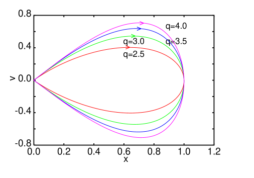
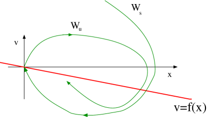
Due to the reflection symmetry of potential (Eq. 3) there are two symmetric solutions for unperturbed homoclinic orbits with ’+’ and ’-’ signs in Eqs. 9-10. A family of right hand side homoclinic orbits has been plotted in Fig. 2. In unperturbed case both stable and unstable manifolds (Poincare sections of the orbits are usually denoted by and ) can be identified with the orbits discussed above while perturbations would influence them in a different way [12]. Existence of cross-sections of between and manifolds signals Smale’s horseshoe scenario of transition to chaos.
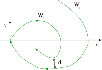
The distance (Fig. 3) between them can be estimated by the Melnikov function :
| (11) |
where the corresponding differential form means the gradient of unperturbed Hamiltonian (Eq. 3):
| (12) |
while is a perturbation form (Eq. 5) to the same Hamiltonian:
| (13) |
All differential forms are defined on homoclinic orbits (Eqs. 9-10).
Thus the Melnikov function :
where and are integrals to be evaluated. appears because of the odd parity of the function under the above integral where
| (15) |
Thus a condition for a global homoclinic transition, corresponding to a hors-shoe type of stable and unstable manifolds cross-section (Fig. 2), can be written as:
| (16) |
For a perturbed system the above constraint together with the explicit form of Melnikov function Eq. 2 gives the critical amplitude :
| (17) |
where and are corresponding integrals given in Eq. 2. In case of we have the following integral
| (18) |
to be evaluated numerically in general but for some cases can be easily performed numerically (see Appendixes B and C) while, in analogy to [16, 17, 18], can be expressed as
| (19) | |||||
where B is the Euler Beta function dependent of arbitrary complex arguments with real parts ( and ) defined as
| (20) |
while denotes the Euler Gamma function:
| (21) |
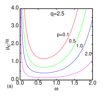
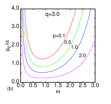
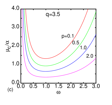
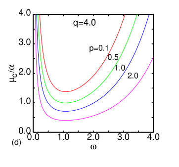
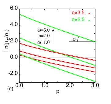
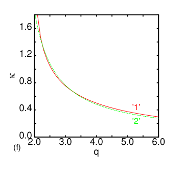
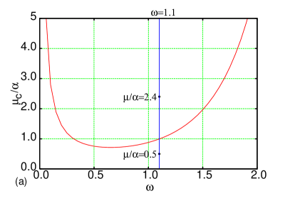
In Fig. 4a–d we plotted the results of Melnikov analysis for a critical amplitude for few values of ( 0.5, 1.0, 2.0) and different ( in Fig. 4a, in Fig. 4b, in Fig. 4c, in Fig. 4d) For the system can transit to chaotic vibrations. Note, in spite of some quantitative changes all four figures (Fig. 4a-d) have similar shape and the sequence of corresponding curves with particular exponents 0.5, 1.0, 2.0 is preserved for any and . This gives us a conviction that may play some independent role. In fact plotting in Fig. 4e versus and we have got straight lines with characteristic slope independent on but changing with . Dependence of the slope :
| (22) |
defined in Fig. 4e, versus has been plotted in Fig. 4f for . Note, the curve ’1’ corresponds to present calculations for while ’2’ is a fitting curve:
| (23) |
The above scaling is not a surprise taking into account the structure of (Eq. 12). In this expression the exponent is entering to the second integral independent of . On can also look into the analytic formulae for in cases of and in the Appendix B (Eq. B.5-B.8) where the appears as an exponent.
3 Results of Numerical Simulations
To illustrate the dynamical behaviour of the system it is necessary to simulate the proper equations. Here we have used the Runge-Kutta method of the forth order and Wolf algorithm [41] to identify the chaotic motion. In our numerical code we started calculations from the same initial conditions for any new examined value of . The system parameters and have be chosen the same as for analytic calculations. We have performed numerical calculations for different choices of system parameters: , , and , hut here, for or technical reasons, we limited our discussion to , , and .
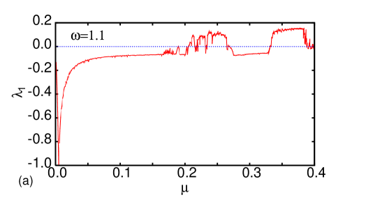
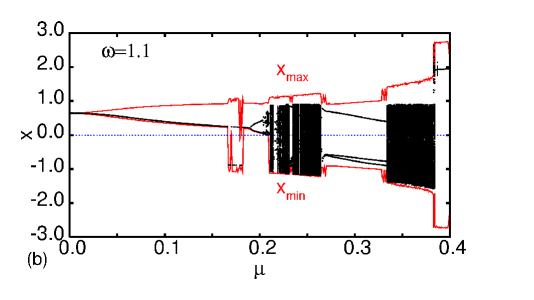
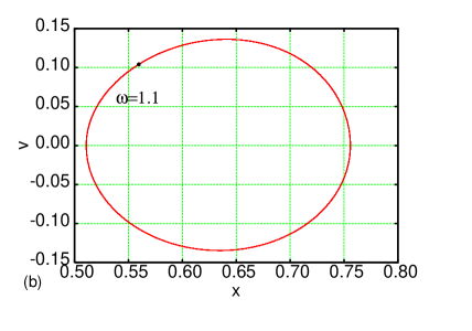
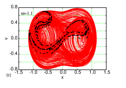
In Fig. 5a we have plotted the maximal Lyapunov exponent versus external forcing amplitude . Here one can clearly see points of sing changes. For and we have got indicating chaotic vibrations. In Fig. 5b we have plotted the corresponding bifurcation diagram. Thus a black region means chaotic motion. This result, as well as others, calculated for different sets of system parameters, is consistent with the Melnikov results. For comparison we have plotted the Melnikov curve again (Fig. 6a with two trial points and (for ). There is no doubt that Fig. 6b shows the regular synchronized motion represented by a single loop on a phase portrait and a singular point on Poincare stroboscopic map. On the other hand Fig. 6c shows clearly a strange attractor of chaotic vibration with complex structure of the Poincare map.
4 Summary and Conclusions
We have examined criteria for transition to chaotic vibrations in the double well system with a damping term described by a fractional exponent and nonlinear potential with negative square term (related negative stiffness) and a positive term with higher exponent where . In spite of non-smoothness of corresponding vector-fields ( and – Eqs. 11 and 12, respectively) it has been proven in the Appendix A that extra terms to the Melnikov integral [40] projected out. Thus the critical value of excitation amplitude above which the system vibrate chaotically has been estimated, in by means of the Melnikov theory [7]. For some selected values of the exponent (4,3, 8/3, 2/5) it was possible to derive a final formula for while for other cases one of Mielnikov’ integrals has be calculated numerically.
The analytical results have been confirmed by simulations. In this approach we used standard methods of analysis as Poincare maps, bifurcation diagrams and Lyapunov exponent.
The Melnikov method, is sensitive to a global homoclinic bifurcation and gives a necessary condition for excitation amplitude system in its transition to chaos [8, 9]. On the other hand the largest Lyapunov exponent [41], measuring the local exponential divergences of particular phase portrait trajectories gives a sufficient condition for this transition which has obviously a higher value of the excitation amplitude .
Above the Melnikov transition predictions () we have obtained transient chaotic vibrations [9, 10, 11, 12, 18] as we expected drifting to a regular steady state away the fractal attraction regions separation boundary. This is typical behaviour of the system which undergo global homoclinic bifurcation.
Acknowledgments
This paper has been partially supported by the Polish Ministry of Science and Information. GL would like to thank Max Planck Institute for the Physics of Complex Systems in Dresden for hospitality.
Appendix A
Starting with the perturbation equation (Eq. 6) we write it in a two element vector form
| (A.1) |
where
| (A.2) | |||||
On the other hand the homoclinic orbit
| (A.3) |
where is usually defined by simple zero of Melnikov integral [7]. In the limit of extreme time the system state reaches a saddle point (see Figs. 1a, 2). Consequently, in the aim to examine the Melnikov criterion for chaos appearance, the vector fields and are defined on the homoclinic orbit (Fig. 2) as:
| (A.4) |
and
| (A.5) |
The perturbed stable and unstable manifolds and read [40]
| (A.6) |
respectively.
Note the perturbation correction to the homoclinic orbit in the above expression (Eq. A.6) should be found by solving the following linear differential equation about the examined time (or a system state ):
| (A.7) |
Note that the above vector fields and are not functions. Namely h is of only if and of if . Similarly g is of only if or and of if and , respectively. In case of the line separates the whole phase space into two parts where is enough smooth (). The same can be applied to the line and as a possible set for and . This line crosses manifold at for the specific time such that and (Fig. A.1).
According to Kunze and Küpper [40] the () space separation includes additional terms to the Melnikov integral.
Thus the Mielnikov function M():
where , are stable and unstable manifold perturbation solutions (Eq. A.7) for in the vicinity of but for ’’ sign and for ’’ sign, respectively.
is defined as for smooth vector fields:
| (A.9) |
and .
Once first discontinuity are identified for , , one have to examine and :
| (A.10) |
and
| (A.11) |
Note substituting for to Eqs. A.10 and A.11 we get the same equations for and consequently the same expressions. This means automatically no extra terms to the Melnikov integral (Eq. Acknowledgments) caused by the discontinuity. Interestingly would lead to a different result but for such case the is no homoclinic orbit in the unperturbed system described by (Eqs. 5,3).
Let us non focus on discontinuity. In this case
| (A.12) |
| (A.13) |
Note, excluding natural odd numbers for the exponent, the above equations (Eqs. A.12 and A.13) are usually different for any other . However both solutions and have to be projected into
| (A.14) |
and the differences in solutions in and are effectively projected out. Interestingly this is also valid for (a dry friction case).
Finally for and the Mielnikov function M() can be treated as a
| (A.15) |
Appendix B
In this appendix we show how to get homoclinic orbits and analytically for some specific cases of exponent : , 3, 2.67 and 2.5.
In case of we follow works by Trueba et al. [16] and Borowiec et al. [18] (and Eqs. 9-10)
| (B.1) |
where ’’ and ’’ signs are related to left– and right–hand side orbits, respectively, is a time like integration constant.
On the other hand for we have
| (B.2) |
Consequently for we have
| (B.3) |
And for
| (B.4) |
The results for a Melnikov integral can be easily found in the above cases. Evaluating the corresponding integral (Eq. 11) after some algebra the last condition (Eq. 16) yields to a critical value of excitation amplitude . Thus for [4, 16, 17, 18] we have:
| (B.5) |
while in case of [42, Litak2005, 43]:
| (B.6) |
for :
| (B.7) |
and finally for :
| (B.8) |
Appendix C
The integral can be evaluated analytically in some specific cases of exponents corresponding to homoclinic orbits Eqs. B.1-B.4 numbered by the corresponding power index applied to hyperbolic function in the denominators. Let us consider integrals for given ,2,3 and 4 related to various exponents , 3, 8/3 and 5/2, respectively. To better clarity we will use new notation for given :
| (C.1) | |||
while constants and are defined as follows:
| (C.2) |
Evaluating the integral (C.1), for positive integer , twice by parts we have got the following recurrence identity
| (C.3) |
Thus only and need to be calculated. Below we evaluate them on the complex plane by summing corresponding residue.
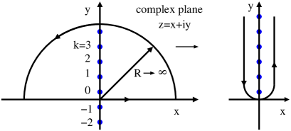
| (C.4) |
where
| (C.5) |
for 1 or 2, in our case.
The examined function is defined as:
| (C.6) |
Note that on the real axis (Fig. C.1) it can be written as
| (C.7) |
The multiplicity of each pole of the complex function (Eq. C.6) is given by
| (C.8) |
Note (Eq. C.1) can be easily determined for or 2. Namely, after summation of all poles in the upper half-plane (Fig. C.1), we get for
| (C.9) |
while for we obtain
| (C.10) |
On the other hand, in case of and (and also for any larger ), we can use the recurrence relation (Eq. C.3):
| (C.11) |
Consequently using Eq. C.1
| (C.12) | |||
References
- [1] Y. Ueda, Randomly Transitional Phenomena in the System Governed by Duffing’s Equation, J. Stat. Phys. 20, 181–196 (1979).
- [2] Y. Ueda, Steady motions exhibited by Duffing’s equations: a picture book of regular and chaotic motions, in New Approaches to Nonlinear Problems in Dynamics, Ed. P.J. Holmes, (SIAM, Philadelphia 1980) pp. 331–322.
- [3] Y. Ueda and N. Akamatsu, Chaotically Transitional Phenomena in the forced negative-resistance oscillator, IEEE Transactions on circuits and Systems 28, 217–224 (1981).
- [4] F.C. Moon and P.J. Holmes, A magetoelastic strange attractor, Journal of Sound and Vibration 65, 275–296 (1979).
- [5] M. Zalalutdinov, K.L. Aubin, M. Pandey, A.T. Zehnder, R.H. Rand, H.G. Craighead, J.M. Parpia, and B.H. Houston, Frequency entrainment for micromechanical oscillator. Applied Phys. Lett. 83, 3281–3283 (2003).
- [6] G. Chong, W. Hai, and Q. Xie, Spatial chaos of trapped Bose Einstein condensate in one-dimensional weak optical lattice potential, Chaos 14, 217–223 (2004).
- [7] V.K. Melnikov, On the stability of the center for time periodic perturbations, Trans. Moscow Math. Soc. 12 1–57 (1963).
- [8] J. Guckenheimer and P. Holmes, Nonlinear oscillations, dynamical systems and bifurcations of vectorfields (Springer, New York 1983)
- [9] S. Wiggins, Introduction to applied nonlinear dynamical systems and chaos (Spinger, New York 1990).
- [10] W. Szemplińska-Stupnicka and J. Rudowski, Bifurcations phenomena in a nonlinear oscillator: approximate analytical studies versus computer simulation results, Physica D 66, 368–380 (1993).
- [11] W. Szemplińska-Stupnicka, The analytical predictive criteria for chaos and escape in nonlinear oscillators: A survey, Nonlinear Dynamics 7, 129–147 (1995).
- [12] E. Tyrkiel, On the role of chaotic saddles in generating chaotic dynamics in nonlinear driven oscillators, Int. J. Bifurcation and Chaos 15, 1215–1238 (2005).
- [13] G. Litak, A. Syta, B. Borowiec, A homoclinic transition to chaos in the Ueda oscillator with external forcing, preprint nlin.CD/0610018, Physica D (2006) submitted.
- [14] F.C. Moon, Chaotic vibrations, an introduction for applied scientists and engineers (John Wiley & Sons, New York 1987).
- [15] G. Litak, G. Spuz-Szpos, K. Szabelski, and J. Warmiński, Vibration analysis of self-excited system with parametric forcing and nonlinear stiffness, Int. J. Bifurcation and Chaos 9, 493–504 (1999).
- [16] J.L. Trueba, J. Rams, and M.A.F. Sanjuan, Analytical estimates of the effect of nonlinear damping in some nonlinear oscillators, Int. J. Bifurcation and Chaos 10, 2257–2267 (2000).
- [17] J.L. Trueba, J.P Baltanás and M.A.F. Sanjuan, Nonlinearly damped oscillators, Recent Res. Devel. Sound & Vibration 1, 29-61 (2002).
- [18] M. Borowiec, G. Litak, A. Syta, Vibration of the Duffing oscillator: Effect of fractional damping, Shock and Vibration 14, 29–36 (2007).
- [19] J. Warmiński, G. Litak, and K. Szabelski, Vibrations of a parametrically and self-excited system with two degrees of freedom in identification in engineering systems, in Proc. of Second International Conference on Identification in Engineering Systems, Swansea, March 1999, Eds. M.I. Friswell, J.M. Mottershead, and A.W. Lees (University of Wales Swansea 1999), pp. 285–294.
- [20] J. Warmiński, G. Litak, and K. Szabelski, Synchronisation and chaos in a parametrically and self-excited system with two degrees of freedom, Nonlinear Dynamics 22, 135–153 (2000).
- [21] R. Lifshitz and M.C. Cross, Response of parametrically driven nonlinear coupled oscillators with application to micromechanical and nanomechanical resonator arrays, Phys. Rev. B 67, 134302 (2003).
- [22] A. Maccari, Parametric excitation for two internally resonant van der Pol oscillators, Nonlinear Dynamics 27, 367–383 (2002).
- [23] A. Maccari, Multiple external excitations for two non-linearly coupled Van der Pol oscillators, J. Sound and Vibr. 259, 967–976 (2003).
- [24] G. Litak, M. Borowiec, A. Syta, and K. Szabelski, Transition to Chaos in the Self-Excited System with a Cubic Double Well Potential and Parametric Forcing, preprint nlin.CD/0601032, Chaos, Solitons & Fractals (2006) submitted.
- [25] J. Awrejcewicz, On the occurrence of chaos in Van der Pol-Duffing oscillator, J. Sound and Vibr. 109, 519–522 (1986).
- [26] M. Siewe Siewe, F.M. Moukam Kakmemi, C. Tchawoua, Resonant oscillation and homoclinic bifurcation in a -Van der Pol oscillator, Chaos, Solitons & Fractals 21, 841–853 (2004).
- [27] R.E. Mickens, K.O. Oyedeji, and S.A. Rucker, Analysis of the simple harmonic oscillator with fractional damping, J. Sound and Vibr. 268, 839–842 (2003).
- [28] H.P.W. Gottlieb, Frequencies of oscillators with fractional power non-linearities, J. Sound and Vibr. 261, 557–566 (2003).
- [29] R.E. Mickens, Fractional Van der Pol Equations, J. Sound Vibr. 259, 457–460 (2003).
- [30] N. M. M. Maia, J. M. M. Silva, and A. M. R. Ribeiro, On general model for damping, J. Sound and Vibr. 218, 749–767 (1998).
- [31] L.-J. Sheu, H.-K. Chen, J.-H. Chen, L.-M. Tam, Chaotic dynamics of the fractionally damped Duffing equation Chaos, Solitons & Fractals 31, 1203–1212 (2007)
- [32] J. Padovan and J.T. Sawicki, Nonlinear Vibration of Fractionally Damped Systems, Nonlinear Dynamics 16 321–336 (1998).
- [33] C.A. Brockley and P.L. Ko, Quasi-harmonic friction–induced vibration. ASME Journal of Lubrication Technology 92, 550–556 (1970).
- [34] R.A. Ibrahim, Friction–induced vibration, chatter, squeal, and chaos. Part I: Mechanics of contact and friction, Appl. Mech. Rev. 47, 209–226 (1994).
- [35] U. Galvanetto and S.R. Bishop, Dynamics of a simple damped oscillator undergoing stick–slip vibrations, Meccanica 34, 337–347 (1999).
- [36] R.I. Leine, D.H. Van Campen, B.L. Van de Vrande, Bifurcations in nonlinear discontinuous systems, Nonlinear Dynamics 23, 105–164 (2000).
- [37] J. Awrejcewicz, M.M. Holicke, Melnikov’s method and stick-slip chaotic oscillations in very weakly forced mechanical systems, Int. J. of Bifurcation and Chaos 9, 505–518 (1999).
- [38] J. Awrejcewicz, Y. Pyryev, Chaos prediction in the Duffing-type system with friction using Melnikov’s function, Nonlinear Analysis: Real World Applications 7, 12–24 (2006).
- [39] J. Awrejcewicz and C.-H. Lamarque, Bifurcation and Chaos in Nonsmooth Mechanical Systems, Series on Nonlinear Science, Series A 45, (World Scientific, Singapore 2003).
- [40] M. Kunze and T. Küpper: Nonsmooth dynamical systems: An overview, in: Ergodic Theory, Analysis, and Efficient Simulation of Dynamical Systems, Ed. B. Fiedler (Springer, Berlin-New York 2001) pp. 431-452.
- [41] A. Wolf, J.B. Swift, H.L. Swinney, and J.A. Vastano, Determining Lyapunov exponents from a time-series, Physica D 16, 285–317 (1985).
- [42] J.M.T. Thompson, Chaotic phenomena triggering the escape from a potential well, Proc. of the Royal Society of London A 421, 195–225 (1989).
- [43] G. Litak, A. Syta, M. Borowiec, Suppression of chaos by weak resonant excitations in a nonlinear oscillator with a non-symmetric potential, Chaos, Solitons & Fractals 32, 694–701 (2007).