Moving and colliding pulses in the subcritical Ginzburg-Landau model with a standing-wave drive

Abstract

We show the existence of steadily moving solitary pulses (SPs) in the complex Ginzburg-Landau (CGL) equation, which includes the cubic-quintic (CQ) nonlinearity and a conservative linear driving term, whose amplitude is a standing wave with wavenumber $k$ and frequency $\omega$, the motion of the SPs being possible at velocities $\pm\omega/k$, which provide locking to the drive. A realization of the model may be provided by traveling-wave convection in a narrow channel with a standing wave excited in its bottom (or on the surface). An analytical approximation is developed, based on an effective equation of motion for the SP coordinate. Direct simulations demonstrate that the effective equation accurately predicts characteristics of the driven motion of pulses, such as a threshold value of the drive’s amplitude. Collisions between two solitons traveling in opposite directions are studied by means of direct simulations, which reveal that they restore their original shapes and velocity after the collision

I Introduction and the model

Complex Ginzburg-Landau (CGL) equations are universal models describing formation of extended patterns and solitary pulses (SPs) in dissipative nonlinear media driven by intrinsic gain. These models are interesting by themselves reviews2 , and also due to their various physical applications. In particular, SP solutions explain the existence of localized pulses observed in traveling-wave convection (TWC) Kolodner , as well as pulsed (soliton) operation regimes featured by fiber lasers laser .

Exact SP solutions are available in the CGL equation with the cubic nonlinearity Lennart , but these pulses are unstable. A straightforward generalization of the model, which makes it possible to create stable SPs, is provided by the cubic-quintic (CQ) nonlinearity. The accordingly modified CGL equation includes linear loss and cubic gain (on the contrary to the linear gain and cubic loss in the cubic equation), and an additional quintic lossy term that provides for the overall stability. The CQ CGL equation was introduced by Petviashvili and Sergeev (in fact, in two dimensions) NizhnyNovgorod , and its stable SP solutions (in one dimension) were first predicted, using an analytical approximation based on the proximity to the nonlinear Schrödinger (NLS) equation, in Ref. PhysicaD . Later, pulses and their stability in the CQ CGL equation were investigated in detail CQCGL ; Hidetsugu .

It is relevant to note that stable SPs may also be found in a model with the cubic nonlinearity only, which is based on the cubic CGL equation linearly coupled to an extra linear dissipative equation Herb-Javid . This system gives rise to exact analytical solutions for stable SPs Javid , and to (numerically found) breathers, i.e., randomly oscillating and randomly walking robust pulses Hidetsugu . In this connection, it is necessary to mention that standing chaotic pulses were found in the CQ CGL equation too DeisslerBrandChaotic , and such pulses were observed experimentally in electrohydrodynamic convection in liquid crystals ExperimentElectroConvChaoticPulse .

A problem of fundamental interest is the understanding of conditions providing for the existence of steadily moving SPs. At the model level, the motion of pulses at arbitrary velocity (and collisions between them) are obviously possible in the CQ CGL equation that does not include a diffusion term HS . In the experiment, pulses persistently moving in either direction, at a very low uniquely determined velocity, were observed in TWC Kolodner . The motion and its extreme slowness were explained by coupling between the CGL equations for the right- left-traveling waves (which can be replaced by a single fourth-order CGL equation Zeitschrift ) and an additional real diffusion-type equation for the concentration field in a binary fluid, where the TWC experiments are performed Riecke .

SPs may be set in persistent motion not only by their intrinsic dynamics, but also by an external drive. In physically relevant situations, this includes a combination of a spatially periodic inhomogeneity – typically, in the form of $\cos(kx)$ – and a time-periodic (ac) driving field applied to the system, in the form of $\cos(\omega t)$. Although the two factors usually act separately (i.e., they appear in different terms of the corresponding equation), the interplay between them naturally suggest a possibility to observe motion of pulses at fundamental resonant velocities, $\pm\omega/k$, and, possibly, also at velocities corresponding to higher spatial and temporal harmonics, i.e., $\pm(m\omega/nk)$, with integer $m$ and $n$.

In models (different from the CGL equations) which give rise to topological solitons, the ac-driven progressive motion of solitons in dissipative media was predicted in both discrete settings (in which case the discreteness itself provides for the periodic spatial inhomogeneity), based on the Toda TL and Frenkel-Kontorova FK lattices, and in continuum models based on modified sine-Gordon equations, that describe weakly damped periodically inhomogeneous ac-driven long Josephson junctions (LJJs) LJJ . Supporting motion of a topological soliton by the ac drive is relatively easy, as the driving field directly couples to the topological charge [in particular, the bias current applied to LJJ directly acts on the magnetic-flux quantum carried by the corresponding topological soliton (fluxon)]. For this reason, the motion of the fluxon in a circular LJJ may also be supported by a rotating magnetic field (i.e., as a matter of fact, by an external traveling wave) applied in the plane of the junction rotating . In all these cases, the ac-driven motion is possible if the amplitude of driving field, $\epsilon$, exceeds a certain threshold value, $\epsilon_{\mathrm{thr}}$ (with $\epsilon<\epsilon_{\mathrm{thr}}$, the traveling-wave drive cannot support the motion of a topological soliton at the velocity equal to the phase velocity of the wave, but it can drag the soliton, supporting its motion in a slow-drift regime drift ).

The predicted modes of the ac-propelled motion of solitons at the resonant velocities were observed experimentally, both in a discrete electric (LC) transmission lattice TL , and in a circular LJJ Ustinov . It is relevant to stress that all the above-mentioned regimes of the ac-driven motion are possible in either direction, hence they are completely different from various soliton ratchets, that have been studied in detail theoretically and experimentally ratchets .

A challenging problem is to find mechanisms making it possible to support persistent motion of nontopological (dynamical) SPs in dissipative media (such as the pulses in CGL models), where the driving force cannot move them directly. Thus far, this was only reported for discrete solitons in a weakly damped Ablowitz-Ladik lattice driven by an ac field AL .

In this work, we aim to demonstrate that such a stable dynamical regime can be found in what may be considered as a paradigmatic model, viz., the CQ CGL equation with an extra conservative term representing a standing wave acting on the system:

$$iu_{t}+\frac{1}{2}u_{xx}+|u|^{2}u=-i\alpha u+i\beta u_{xx}+i\gamma|u|^{2}u-i\Gamma|u|^{4}u-\epsilon\cos\left(kx\right)\cos\left(\omega t\right)u,$$ (1)

Coefficients $\alpha\geq 0,\beta\geq 0$ and $\gamma>0,\Gamma>0$ on the right-hand side of Eq. (1) account for the linear loss, effective diffusion, cubic gain, and quintic loss, respectively. Using the scale invariance of Eq. (1), we will fix $k\equiv 1/4$, while $\epsilon$ and $\omega$ remain arbitrary parameters.

A straightforward physical realization of Eq. (1) can be found in terms of TWC (in a binary fluid), which, as said above, is adequately modeled (in the region of the subcritical instability) by the CQ CGL Kolodner . The driving term, which is a conservative one [i.e., it yields zero contribution to the balance equation for the norm, see Eq. (4) below], may be generated by a standing elastic (acoustic) wave created on the bottom of the convection cell (or, possibly, a standing wave created on the surface of the convection layer), provided that the drive’s wavelength, $2\pi/k$, is much larger than the critical wavelength of the convection-triggering instability, and $\omega$ must be sufficiently small too. The latter conditions comply with the analysis developed below, which is focused on the case of $k/\eta\ll 1$, and needs to have $\omega$ small enough too, to provide for a reasonably small locking threshold, see Eqs. (9) and (10) below.

The coefficient in front of the driving term in Eq. (1) can be decomposed into a superposition of two counter-propagating traveling waves,

$$\cos\left(kx\right)\cos\left(\omega t\right)=\frac{1}{2}\left[\cos\left(k\left(x-c_{0}t\right)\right)+\cos\left(k\left(x+c_{0}t\right)\right)\right],$$ (2)

where $c_{0}\equiv\omega/k$. As said above, this decomposition suggests that the drive may support motion of a soliton with either positive or negative resonant velocity, $c=\pm c_{0}$. However, the actual existence of stable moving solitons, locked to either traveling-wave component of the drive, is not obvious. An objective of this work is to predict this possibility in an analytical approximation, and verify it by numerical simulations of Eq.(1), identifying a parameter region in which SPs can steadily move at the resonant velocity (slow drift of driven pulses is formally possible too, but it turns out to be always unstable, in the present model).

The analytical and numerical findings are presented below in Sections II and III, respectively. In concluding Section IV, we summarize the obtained results.

II Analytical approximation

Equation (1) is written in the form of a perturbed nonlinear Schrödinger (NLS) equation, which, in the absence of perturbations ($\alpha=\beta=\gamma=\Gamma=\epsilon=0$), has a family of ordinary soliton solutions,

$$u_{\mathrm{sol}}=\eta~{}\mathrm{sech}\left(\eta(\left[x-\xi(t)\right]\right)~{}e^{icx+(i/2)\left(\eta^{2}-c^{2}\right)t},\quad~{}\dot{\xi}=c,$$ (3)

with arbitrary amplitude $\eta$ and velocity $c$ (the overdot stands for $d/dt$). For $\epsilon=0$ (no driving term), but with $\alpha,\beta,\gamma,\Gamma>0$, two stationary solitons are selected from continuous family (3) by the norm-balance condition,

$$\frac{d}{dt}\left(\int_{-\infty}^{+\infty}|u(x)|^{2}dx\right)=0.$$ (4)

Within the framework of the perturbation theory, Eq. (4) yields the following values of the amplitude PhysicaD :

$$\eta_{\pm}^{2}=\frac{5\left(2\gamma-\beta\right)\pm\sqrt{5\left[5\left(2\gamma-\beta\right)^{2}-96\alpha\Gamma\right]}}{16\Gamma},$$ (5)

while the velocity is zero. The pulses corresponding to larger and smaller values given by Eq. (5), i.e., $\eta_{+}$ and $\eta_{-}$, are stable and unstable, respectively.

To proceed with the analytical approach for $\epsilon\neq 0$, we make use of the balance equation for the momentum, $P=i\int_{-\infty}^{+\infty}u_{x}^{\ast}udx$, with asterisk standing for the complex conjugate. Indeed, an exact corollary of Eq. (1) is

$$\frac{dP}{dt}=-2\alpha P-\beta\int_{-\infty}^{+\infty}i\left(u_{x}u_{xx}^{\ast}-u_{x}^{\ast}u_{xx}\right)dx$$

$$+\int_{-\infty}^{+\infty}\left(\gamma|u|^{2}-\Gamma|u|^{4}\right)i\left(u_{x}u_{xx}^{\ast}-u_{x}^{\ast}u_{xx}\right)dx-\epsilon k\cos(\omega t)\int_{-\infty}^{+\infty}\sin(2kx)\cdot|u|^{2}dx~{}.$$ (6)

In the spirit of the multiscale perturbation theory, we assume that the loss and gain terms in Eq. (1) represent stronger perturbations, hence they select value (5), with the upper sign, for $\eta$. Strictly speaking, the use of that expression implies that the velocity is small enough, $\dot{\xi}^{2}\ll\eta_{+}^{2}$ [then, an additional contribution to the norm-balance equation (4) for the moving solitons, $\sim\beta\dot{\xi}^{2}$, may be neglected]. After that, the substitution of expression (3) with the constant amplitude, $\eta=\eta_{+}$, in Eq. (6) and straightforward integrations yield the following effective equation of motion for the central coordinate, $\xi(t)$ (we omit the subscript in $\eta_{+}$):

$$\ddot{\xi}=-\frac{4}{3}\beta\eta^{2}\dot{\xi}-2\beta\dot{\xi}^{3}-\frac{\pi\epsilon k^{2}}{2\eta\sinh\left(\pi k/2\eta\right)}\sin\left(k\xi\right)\cos(\omega t).$$ (7)

In the case of narrow solitons, $k/\eta\ll 1$, Eq. (7) simplifies:

$$\ddot{\xi}=-\frac{4}{3}\beta\eta^{2}\dot{\xi}-2\beta\dot{\xi}^{3}-\epsilon k\sin\left(k\xi\right)\cos(\omega t).$$ (8)

Equation (8) with $\epsilon=0$ (no drive) admits an explicit analytical solution:

$$\dot{\xi}^{2}(t)=\frac{2}{3}\frac{\eta^{2}}{\left(1+2\eta^{2}/3\dot{\xi}_{0}^{2}\right)\exp\left(3t/2\beta\eta^{2}\right)-1}.$$

In the presence of the drive, motion at the average velocity $c_{0}$ implies the existence of a solution to Eq. (7) in the form of $\xi(t)=c_{0}\left(t-t_{0}\right)+\Xi(t)$, with some constant $t_{0}$ and time-periodic terms $\Xi(t)$. Applying to Eq. (7) known methods used in the analysis of the ac-driven motion of solitons at the resonant velocity TL - rotating , we conclude that, in the present case, the ac-propelled resonant motion may be possible, provided that the drive’s amplitude exceeds a threshold value,

$$\epsilon>\epsilon_{\mathrm{thr}}=\frac{8\beta\omega\eta\left(2\eta^{2}k^{2}+3\omega^{2}\right)}{3\pi k^{5}}\sinh\left(\frac{\pi k}{2\eta}\right).$$ (9)

Actually, the threshold is identified as the smallest value of $\epsilon$ at which the average value of the last (driving) term on the right-hand side of Eq. (7) may compensate the first two (braking) terms, with $\dot{\xi}=\omega/k$. For narrow solitons, with $k/\eta\ll 1$, expression (9) simplifies,

$$\epsilon>\epsilon_{\mathrm{thr}}=\frac{4\beta\omega}{3k^{4}}\left(2\eta^{2}k^{2}+3\omega^{2}\right).$$ (10)

As mentioned above, in the case of $\epsilon<\epsilon_{\mathrm{thr}}$ one may consider a drift regime, in which the SP is dragged by either traveling wave from Eq. (2) at a small velocity, $c\ll c_{0}$. However, additional analytical considerations, as well as direct simulations, demonstrate that the drift mode of motion is always unstable in the present system (unlike the resonant-motion regime, which may definitely be stable).

As shown in Fig. 1, we have compared analytical prediction (9) for the threshold amplitude with findings following from simulations of Eq. (7). The results are in good agreement for low dissipation rates, and the agreement deteriorates with the increase of $\beta\eta^{2}$, which is quite natural, as the perturbation theory is based on the assumption of weak dissipation. Generally, analytical expression (9) underestimates the actual threshold.

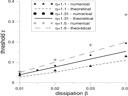
Figure 1: Comparison of the numerical results (symbols) and the theoretical prediction, given by Eq. (9) (lines), for the minimum amplitude of the external drive $\epsilon$ necessary to support a steady traveling solution in Eq. (7). Here and in all examples displayed below, the driving wave is taken with $k=0.25$ and $\omega=0.05$.

A typical example of the dependence of the established ac-driven regimes of motion [as per effective equation of motion (7)] on initial values of the coordinate and velocity is displayed in Fig. 2. For the explored parameter range, simulations of Eq. (7) demonstrate that the motion regimes corresponding to the fundamental-resonance velocities, $\pm\omega/k$, are the single stable states (attractors) for $\epsilon>\epsilon_{\mathrm{thr}}$ (velocities corresponding to the locking of a moving SP to higher-order resonances do not emerge in the simulations), while only the states with zero average velocity are stable for $\epsilon<\epsilon_{\mathrm{thr}}$. Despite the interweaving attraction basins of the two stable regimes, which is quite a notable feature of Fig. 2, the simulations of Eq. (7) do not reveal any hysteresis in the established states (i.e., no overlap between the two attraction basins).

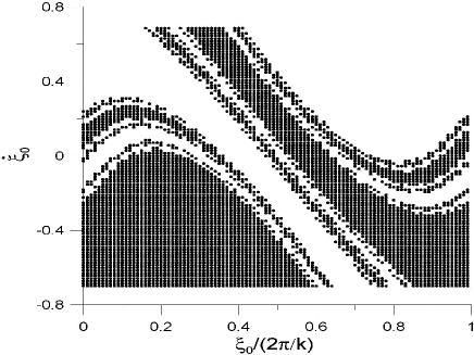
Figure 2: Results of the numerical integration of the equation of motion, Eq. (7), with $\beta=0.02$, $\epsilon=0.1$, and $\eta=1.31$, obtained by varying initial values of the coordinate and velocity, $\xi_{0}$ and $\dot{\xi}_{0}$. White space and black dots denote, respectively, established states in the form of the motion with resonance velocities $c_{0}=+0.2$ and $-0.2$, respectively.

III Numerical simulations of the complex Ginzburg-Landau equation

III.1 Verification of the ac-driven regime of motion

To verify and expand the predictions of the analytical approach developed in the previous section, we have performed direct numerical simulations of the underlying PDE, i.e., the driven CQ CGL equation, Eq. (1). First, we have evaluated the amplitude of the soliton for a given set of gain and loss parameters in the CQ CGL equation (1) with $\epsilon=0$, using the above analytical predictions. For instance, Eq. (5) with $\alpha=0.01$, $\beta=0.02$, $\gamma=0.06$, and $\Gamma=0.03$ predicts the stable soliton’s amplitude, $\eta_{+}=1.31$. Next, we have estimated the threshold strength, $\epsilon_{\mathrm{thr}}$, of the ac drive in Eq. (1). Taking (as in the above examples) $k=0.25$ and $\omega=0.05$, which correspond to resonance velocity $c_{0}\equiv\omega/k=0.2$, Eq. (9) yields $\epsilon_{\mathrm{thr}}=0.077$. The spatial period (i.e., $k$) was selected so as to minimize excitation of internal vibrations in the SP under the action of the driving term. To this end, narrow pulses were chosen, with $\eta k\ll 1$ [note this is the same assumption which made it possible to simplify Eq. (7), replacing it by Eq. (8), and Eq. (9) by Eq. (10)].

In Fig. 3 we display the simulated evolution of the SP which was initially placed at position $\xi_{0}=16\pi$ and set in motion with the initial velocity $c_{0}=-0.2$. If the driving potential strength is below the threshold value, $\epsilon<\epsilon_{\mathrm{thr}}$, the SP gets trapped within a finite domain, as seen in the left panel of Fig. 3; on the other hand, simulations of Eq. (1) with $\epsilon>\epsilon_{\mathrm{thr}}$ reveal, as expected, stable motion of the solitary pulse, see the right panel of Fig. 3.

 

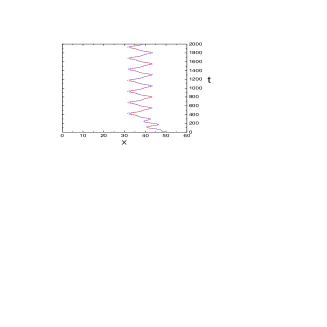
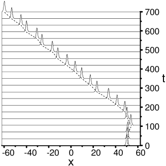
Figure 3: (Color online) Soliton with amplitude $\eta=1.31$ is set, at $t=0$, at point $\xi_{0}=16\pi$, and shoved by lending it initial velocity $c_{0}=-0.2$ [in fact, it means amplifying the soliton by $\exp(ic_{0}x)$]. The coefficients in Eq. (1) are $\alpha=0.01$, $\beta=0.02$, $\gamma=0.06,$ $\Gamma=0.03$, and $\omega=0.05,k=0.25$. Left panel: The motion of the soliton’s center as predicted by Eq. (7) (blue dashed line), and as found from the direct simulations of the full CGL equation, Eq. (1) (red continuous line). When the strength of the driving force is smaller than the threshold value, e.g., $\varepsilon=0.05\$[recall Eq. (9) predicts $\varepsilon_{\mathrm{thr}}=0.077$ for the present case], consistent motion of the solitary pulse does not occur. Right panel: When the strength of the driving force exceeds the threshold, e.g., $\varepsilon=0.1>\varepsilon_{\mathrm{thr}}$, the soliton moves steadily, as expected. In the picture, we juxtaposed a series of the soliton’s profiles extracted from the numerical solution of Eq. (1), with the trajectory of motion predicted by Eq. (7) (dashed line).

Systematic simulations of Eq. (1) corroborate the predictions of the analytical approach based on Eq. (7). We did not aim to find the threshold value of the drive’s amplitude from the PDE simulations with a very high accuracy, but, generally, the numerical results are in accordance with the above prediction given by Eq. (9).

III.2 Collisions between solitary pulses

The existence of stably moving ac-propelled SPs suggest a possibility to consider collisions between them. Figure 4 displays a simulated collision of two identical pulses moving with opposite velocities, $c_{0}=\pm 0.2$, both being driven by the standing wave with $\epsilon=0.1$. This and other runs of the simulations demonstrate that the solitons survive the collision. As seen from Fig. 4, each soliton readily recovers its original shape and velocity after the collision, which is easily explained by the fact that these shapes and velocities correspond to unique attractors of the ac-driven CQ CGL equation, see above. A generic feature obvious in Fig. 4 and observed in many other runs of simulations is that multiple collisions actually occur between the moving pulses.

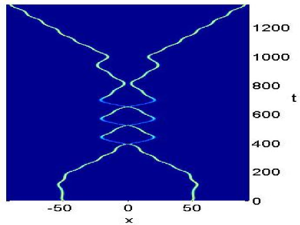
Figure 4: (Color online) Collision of two ac-driven solitary pulses with opposite velocities, $c_{0}=\pm 0.2$. After a series of repeated collisions, the pulses eventually separate, completely restoring their initial shape and velocities. Parameters are the same as in the right panel of Fig. 3.

The collisions are additionally illustrated, in Fig. 5, by plots showing the norm and amplitude of the colliding pulses as functions of time. It is seen that the total norm undergoes violent changes when the collision takes place, but later it quickly recovers the original value. No tangible radiation coming out from the collision region have be found in the simulations.

Figure 5: Time dependencies of the amplitude of the wave field ($A$) and its total norm ($N$) additionally illustrating the collision between two solitary pulses shown in Fig. 4.

IV Conclusion

In this paper, we have shown that solitary pulses in the cubic-quintic CGL equation which contains the conservative standing-wave driving term can lock to the resonant velocities provided by the drive, and thus move to right or left in a stable fashion. This dynamical regime was predicted in an analytical form, by means of the effective equation of motion for coordinate of the solitary pulse, and corroborated by direct simulations of the full CGL equation, with the driving term. In particular, the threshold value of the drive’s amplitude (the minimum amplitude necessary to lock the pulse to the resonant velocity), which was predicted by the effective equation of motion, is quite close to values provided by the full simulations. Unlike the motion mode with the velocity corresponding to the fundamental resonance with the external drive, motion of a pulse locked to a higher-order resonance is never observed, nor is a dragging (slow-drift) mode ever found. Collision between ac-driven pulses moving in opposite directions were also studied, by means of the direct simulations. It was concluded that the solitary pulses are robust in this sense too, recovering the initial shapes and velocities after the collision.

References

- (1) I. S. Aranson, L. Kramer, Rev. Mod. Phys. 74, 99 (2002); B. A. Malomed, in: Encyclopedia of Nonlinear Science, p. 157 (ed. by A. Scott; New York, Routledge, 2005).
- (2) P. Kolodner, Phys. Rev. A 44, 6448 (1991); A. C. Newell, T. Passot, and J. Lega, Ann. Rev. Fluid Mech. 25, 399 (1993); P. Kolodner, S. Slimani, N. Aubry, and R. Lima, Physica D 85, 165 (1995).
- (3) F. O. Ilday, F. W. Wise, J. Opt. Soc. Am. B 19, 470 (2000); Y. D. Gong, P. Shum, D. Y. Tang, C. Lu, X. Guo, V. Paulose, W. S. Man, H. Y. Tam, Opt. Laser Technology 36, 299 (2004).
- (4) L. M. Hocking and K. Stewartson, Proc. Roy. Soc. L. A 326, 289 (1972); N. R. Pereira and L. Stenflo, Phys. Fluids 20, 1735 (1977).
- (5) V. I. Petviashvili and A. M. Sergeev, Dokl. AN SSSR 276, 1380 (1984) [Sov. Phys. Doklady 29, 493 (1984)].
- (6) B. A. Malomed, Physica D 29, 155 (1987).
- (7) O. Thual and S. Fauve, J. Phys. (Paris) 49, 1829 (1988); S. Fauve and O. Thual, Phys. Rev. Lett. 64, 282 (1990); W. van Saarloos and P. C. Hohenberg, Phys. Rev. Lett. 64, 749 (1990); B. A. Malomed and A. A. Nepomnyashchy, Phys. Rev. A 42, 6009 (1990); V. Hakim, P. Jakobsen and Y. Pomeau, Europhys. Lett. 11, 19 (1990); P. Marcq, H. Chaté, and R. Conte, Physica D 73, 305 (1994); J. M. Soto-Crespo, N. N. Akhmediev, and V. V. Afanasjev, J. Opt. Soc. Am. B 13, 1439 (1996); O. Descalzi, M. Argentina and E. Tirapegui, Phys. Rev. E 67 , 015601(R) (2003).
- (8) B. A. Malomed and H. G. Winful, Phys. Rev. E 53, 5365 (1996); J. Atai and B. A. Malomed, Phys. Rev. E 54, 4371 (1996).
- (9) J. Atai and B. A. Malomed, Phys. Lett. A 246, 412 (1998).
- (10) H. Sakaguchi and B. A. Malomed, Physica D 147, 273 (2000); ibid. 154, 229 (2001).
- (11) R. J. Deissler and H. R. Brand, Phys. Rev. Lett. 72, 478 (1994).
- (12) M. Dennin, G. Ahlers, and D. S. Cannell, Phys. Rev. Lett. 77, 2475 (1996).
- (13) B. A. Malomed, Zs. Phys. B 55, 241 (1984); ibid. 55, 249 (1984).
- (14) H. Sakaguchi, Physica D 210, 138 (2005).
- (15) H. Riecke, Phys. Rev. Lett. 68, 301 (1992); Physica D 61, 253 (1992).
- (16) B. A. Malomed, Phys. Rev. A 45, 4097 (1992); T. Kuusela, J. Hietarinta, and B. A. Malomed, J. Phys. A 26, L21 (1993); K. D. Rasmussen, B. A. Malomed, A. R. Bishop, and N. Grønbech-Jensen, Phys. Rev. E 58, 6695 (1998).
- (17) L. L. Bonilla and B. A. Malomed, Phys. Rev. B 43, 11539 (1991); G. Filatrella and B. A. Malomed, J. Phys. Cond. Matter 11, 7103 (1999).
- (18) G. Filatrella, B. A. Malomed, and R. D. Parmentier, Phys. Lett. A 180, 346 (1993); ibid. 198, 43 (1995); G. Filatrella, B. A. Malomed, R. D. Parmentier, and M. Salerno, ibid. 228, 250 (1997).
- (19) N. Grønbech-Jensen, B. A. Malomed, and M. R. Samuelsen, Phys. Rev. B 46, 294 (1992).
- (20) B. A. Malomed, J. Phys. Soc. Jpn. 62, 997 (1993).
- (21) T. Kuusela, Phys. Lett. A 167, 54 (1992).
- (22) A. V. Ustinov and B. A. Malomed, Phys. Rev. B 64, 020302(R) (2001).
- (23) F. Marchesoni, Phys. Rev. Lett. 77, 2364 (1996); A. V. Savin, G. P. Tsironis, and A. V. Zolotaryuk, Phys. Rev. E 56, 2457 (1997); E. Goldobin, A. Sterck, and D. Koelle, ibid. 63, 031111 (2001); M. Salerno and N. R. Quintero, ibid. 65, 025602 (2002); S. Flach, Y. Zolotaryuk, A. E. Miroshnichenko, and M. V. Fistul, Phys. Rev. Lett. 88, 184101 (2002); L. Morales-Molina, N. R. Quintero, F. G. Mertens, and A. Sanchez, ibid. 91, 234102 (2003); A. V. Ustinov, C. Coqui, A. Kemp, Y. Zolotaryuk, and M. Salerno, ibid. 93, 087001 (2004).
- (24) D. Cai, A. R. Bishop, N. Grønbech-Jensen, and B. A. Malomed, Phys. Rev. E 50, R694 (1994).