Inverse turbulent cascades and conformally invariant curves

Abstract

We offer a new example of conformal invariance far from equilibrium — the inverse cascade of Surface Quasi-Geostrophic (SQG) turbulence. We show that temperature isolines are statistically equivalent to curves that can be mapped into a one-dimensional Brownian walk (called Schramm-Loewner Evolution or SLE_κ). The diffusivity is close to $\kappa=4$, that is iso-temperature curves belong to the same universality class as domain walls in the $O(2)$ spin model. Several statistics of temperature clusters and isolines are measured and shown to be consistent with the theoretical expectations for such a spin system at criticality. We also show that the direct cascade in two-dimensional Navier-Stokes turbulence is not conformal invariant. The emerging picture is that conformal invariance may be expected for inverse turbulent cascades of strongly interacting systems.

To identify underlying symmetries is a central problem of the statistical physics of infinite-dimensional strongly fluctuating systems. Turbulence is a state of such a system which is deviated far from equilibrium and is accompanied by dissipation. Excitation and dissipation usually break symmetries such as scale invariance, isotropy and time reversibility. In fully developed turbulence, the scales of excitation and dissipation differ strongly and are separated by the so-called inertial interval. The main fundamental problem of turbulence is how universal is the statistics of fluctuations in the inertial interval FS . Are symmetries, broken by excitation and dissipation, eventually restored in that range Pol ? Cascades can be direct or inverse depending on whether the integral of motion is transferred towards small or large scales, respectively. Symmetries broken by excitation (scale invariance and isotropy) are generally not restored in direct cascades due to the existence of statistically conserved quantities FS ; FGV . On the contrary, symmetries are expected to be restored in the inverse cascade where one looks at scales much larger than the pumping scale. This is consistent with the observation that inverse cascades are scale invariant BCV00 ; Tab ; CCMV . Moreover, it has been shown recently that the statistics of zero-vorticity lines in the inverse cascade of two-dimensional (2d) Navier-Stokes turbulence display conformal invariance (i.e. local scale invariance), revealing an unexpected connection with percolation BBCF06 . Such tantalizing results, while awaiting a theory capable of explaining them from first principles, pose new questions: Are there other turbulent flows that share this property and do they belong to the same universality class of percolation? In this Letter we answer them by a numerical investigation of SQG turbulence. This system is relevant for geophysical applications HPGS95 and qualitatively similar to Navier-Stokes 2d turbulence. We show that zero-temperature isolines are SLE₄ curves at large scales (in the inverse cascade). Therefore, the isolines belong to the same universality class as the trace of a harmonic explorer, certain isolines of a Gaussian (free) field SS , interfaces in the $O(2)$ model and frontiers of Fortuin-Kasteleyn clusters in the $4-$state Potts model at the critical point (for an introduction to SLE and statistical models see Refs. C05 ; BB06 and references therein). This connection allows to obtain analytical predictions for some characteristic exponents of cluster and loop statistics that compare well with numerical results.

The SQG model describes a rotating stably stratified fluid with a uniform potential vorticity HPGS95 . The temperature is advected along a surface bounding a constant potential vorticity interior,

$$\partial_{t}T+{\bm{v}}\cdot{\bm{\nabla}}T=\varkappa\nabla^{2}T+f\,,$$ (1)

and determines the velocity ${\bm{v}}=\hat{\bm{z}}\times{\bm{\nabla}}\psi$, $\psi({\bm{x}},t)=\int d{\bm{y}}\,|{\bm{x}}-{\bm{y}}|^{-1}T({\bm{y}},t)$. Without dissipation and forcing ($\varkappa=f=0$) the equations admit two positive-defined quadratic invariants $Z=\int T^{2}d{\bm{x}}$ and $E=\int\psi Td{\bm{x}}$. In the presence of a forcing that injects temperature fluctuations at a scale $l_{f}$, a double cascade develops, akin to the one observed in 2d Navier-Stokes turbulence: the “energy” $E$ flows upscales whereas the “enstrophy” $Z$ goes downscales. Here we focus on the inverse cascade. Requiring the energy flux to be scale independent one gets the scaling law $\delta_{r}T=T({\bm{x}}+{\bm{r}})-T({\bm{x}})\sim r^{H}$ with $H=0$ (i.e. logarithmic correlation functions). Indeed, numerical simulations show that the temperature field in the inverse cascade displays a self-similar statistics with a scaling compatible with dimensional expectations (see HPGS95 ; PHS94 ; S00 ; SBHMTHV02 ; CCMV04 and Fig. 1).

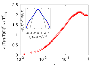
Figure 1: The second-order structure function of temperature differences and, in the inset, probability density functions for $r=0.02,0.04,0.06$ compared to a Gaussian density (solid line). Data have been obtained by a direct numerical simulations of (1) by a pseudo-spectral code in a fully periodic, square domain of size $1$ with $4096^{2}$ lattice points. Gaussian white-in-time forcing $f$ has correlation length $l_{f}\approx 1/200$. The system is kept in a statistically stationary state by supplementing (1) with a linear damping term $-T/\tau$ that models bottom friction and extracts energy at very large scales $l_{\tau}\propto\tau$, ($l_{\tau}=1/20\div 1/10$ depending on $\tau$).

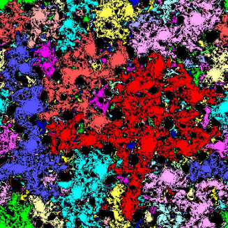
Figure 2: Temperature clusters in the inverse cascade of SQG turbulence. These are connected domains with positive temperature. Negative temperature regions are black.

We now consider the connected regions of like-sign temperature (clusters) and their boundaries (loops) — see Fig. 2. To guess the cluster statistics one needs the knowledge of the scaling properties of the temperature field. Indeed, for a self-similar field with Hurst exponent $H=0$ the fractal dimension of loops is $3/2$ KH95 . If one assumes that such loop ensemble has a conformal invariant scaling limit, it should belong to the same universality class as loops in the $O(2)$ model in the dense phase. By exploiting the Coulomb gas representation of the latter system (with $g=1$, N84 ) and general scaling arguments KH95 it is possible to derive analytically a set of scaling exponents associated to cluster and loop statistics. These include the fractal dimensions of clusters and loops, the power-law exponents for the number of clusters of given mass and the number of loops of given length, radius of gyration, or area. In Figure 3 such statistics are displayed for Surface Quasi-Geostrophic turbulence and shown to be consistent with that of $O(2)$ model.

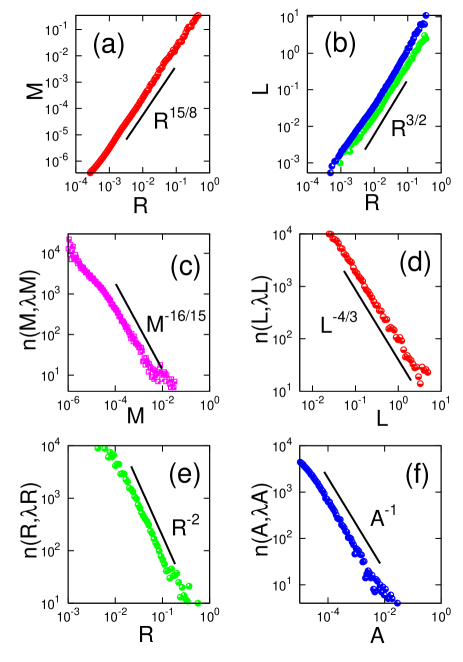
Figure 3: Cluster and loop statistics for SQG turbulence. (a) The average area $M$ versus the radius of gyration $R$. (b) The length of a loop (blue symbols) and its externally accessible perimeter which is obtained by subtraction of fjords with necks smaller than $l_{f}$ (green symbols) versus $R$. (c) Number of clusters of area between $M$ and $\lambda M$. (d) Number of loops of length between $L$ and $\lambda L$. (e) Number of loops of radius between $R$ and $\lambda R$. (f) Number of loops of area between $A$ and $\lambda A$. In all figures $\lambda\simeq 1.1$. The solid lines are the theoretical expectations for the $O(2)$ model.

These results give a strong indication that loops, i.e. zero-temperature isolines, might be conformally invariant objects. If this is the case they should be statistically equivalent to SLE_κ curves with the diffusivity $\kappa=4$, as it is conjectured for the $O(2)$ model. To verify directly this hypothesis, we proceeded as follows. First, we identify putative SLE traces. After having isolated zero-field lines, a walker follows them as they explore the upper-half plane. The search ends when the walker touches the real axis at a distance from the origin larger than $l_{\tau}$. A sample trace is shown in Figure 4 (a). This selection procedure, self-consistent for $\kappa\leq 4$, yields a set of curves in the half-plane, which are expected in the scaling limit to converge to chordal SLE joining two points on the real axis. Second, we extract the Loewner driving function from the trace. To this aim, let us consider chordal SLE in the upper-half plane $H$ from $0$ to $x_{\infty}$. We parametrize the curve by the dimensionless $t$, not to be confused with time in (1). The equation for $g_{t}(z)$ which maps the half-plane minus the trace up to $t$ into $H$ itself, is $\partial_{t}g_{t}=2/\{\varphi^{{}^{\prime}}(g_{t})[\varphi(g_{t})-\xi_{t}]\}$ where $\varphi(z)=x_{\infty}z/(x_{\infty}-z)$. The equation for $g_{t}$ can be solved for a constant $\xi$: $G_{t,\,\xi}(z)=x_{\infty}\{\eta x_{\infty}(x_{\infty}-z)+[x_{\infty}^{4}(z-\eta)^{2}+4t(x_{\infty}-z)^{2}(x_{\infty}-\eta)^{2}]^{1/2}\}/\{x_{\infty}^{2}(x_{\infty}-z)+[x_{\infty}^{4}(z-\eta)^{2}+4t(x_{\infty}-z)^{2}(x_{\infty}-\eta)^{2}]^{1/2}\}$ where $\eta=\varphi^{-1}(\xi)$. In this case the trace is the semicircle joining $\eta$ and $x_{\infty}$.

Figure 4: (a) A putative SLE trace. (b) A cartoon of the algorithm used to extract the driving function from the trace (see text). The procedure has been checked on an ensemble of self-avoiding loops where it yielded the correct value $\kappa=8/3$ with an uncertainty of less than 5%.

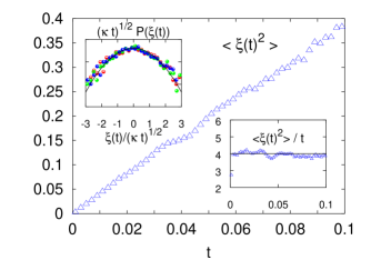
Figure 5: Statistics of the driving function. In the main frame is shown the diffusive behavior of $\xi(t)$. Lower-right inset: the diffusion coefficient is $\kappa=4\pm 0.2$. Upper-left inset: the probability density of $\xi_{t}$, rescaled by its variance is Gaussian (different symbols correspond to $t=0.02,0.04,0.08$).

For a generic $\xi(t)$ we partition the interval $[0,T]$ into subintervals $[t_{n},t_{n+1})$ with $t_{0}=0$, $t_{N+1}=T$ where we approximate the driving function by the constant $\xi_{n}=\xi(t_{n})$ and express $g_{t}$ as a composition $G_{t_{N}-t_{N-1},\,\xi_{N-1}}\circ\cdots\circ G_{t_{1},\,\xi_{0}}$. It is now possible to extract the driving function from a candidate SLE trace, approximated by a sequence of points $\{z_{0},z_{1},\ldots,z_{N+1}\}$, where $z_{0}=0$ and $z_{N+1}=x_{\infty}$. The first step is to identify the unique semicircle passing through the points $x_{\infty}$ and $z_{1}$ [see Fig. 4 (b) for an illustration]. This yields the values for $\eta_{0}=\varphi^{-1}(\xi_{0})=\left[\mathrm{Re}z_{1}\,x_{\infty}-(\mathrm{Re}z_{1})^{2}-(\mathrm{Im}z_{1})^{2}\right]/(x_{\infty}-\mathrm{Re}z_{1})$ and $t_{1}=(\mathrm{Im}z_{1})^{2}x_{\infty}^{4}/\{4[(\mathrm{Re}z_{1}-x_{\infty})^{2}+(\mathrm{Im}z_{1})^{2}]^{2}\}$. The map $G_{t_{1},\,\xi_{0}}$ is then applied to the points resulting in a new sequence, by one element shorter: $z^{\prime}_{k}=G_{t_{1},\,\xi_{0}}(z_{k+1})$ with $k=1\ldots N$. The operation is iterated on the new subsequence of points until one obtains the full set of $t_{k}$ and $\xi_{k}$ that gives a piecewise constant approximation of the driving function.

The result of this procedure is an ensemble of $\xi(t)$ whose statistics converge, for $l_{f}^{2}\!\lesssim\!\kappa t\!\lesssim\!l_{\tau}^{2}$ to a Gaussian process with the variance $\langle\xi^{2}(t)\rangle\!=\!\kappa t$ and $\kappa\!=\!4\!\pm 0.2$, as shown in Figure 5. We conclude that, within statistical errors, zero-temperature isolines in the inverse cascade of SQG turbulence are locally SLE₄ curves. This applies also to other $T$ contours provided that $T\ll T_{rms}$. Moreover, in the limit of very large system size where $T({\bm{r}})$ tends to a self-affine field and $T_{rms}$ diverges, we expect all iso-level loops to be statistically equivalent (another application of SLE to non-equilibrium systems has been found recently for spin glasses Hast ).

Remark that Surface Quasi-Geostrophic and Navier-Stokes systems belong to a class that is uniquely specified by the transport equation (1) and by a linear, scale-invariant, local in time relationship between the advected field and the streamfunction $\psi({\bm{x}},t)=\int d{\bm{y}}\,|{\bm{x}}-{\bm{y}}|^{\alpha-2}T({\bm{y}},t)$ PHS94 . SQG dynamics corresponds to $\alpha=1$, Navier-Stokes equation to $\alpha\to 2$, $T$ being vorticity. The large-scale limit of the Charney-Hasegawa-Mima model CHM , relevant for atmospheric and plasma turbulence, corresponds to $\alpha=-2$. Dimensional arguments for the inverse cascade in this class of models give $\delta_{r}T\propto r^{H}$ with $H=(2-2\alpha)/3$. This exponent can be used to infer the dimension of the contour loops $(3-H)/2=(7+2\alpha)/6$ KH95 (for $0<H<1$ and $-1/2<\alpha<1$) and thus conjecture that they converge to SLE_κ curves with $\kappa=4(1+2\alpha)/3$.

Let us stress that the temperature field in our model has non-Gaussian statistics, see CCMV04 and Fig. 1. A similar non-Gaussian form with logarithmic moments holds for the height function built on independently oriented loops from the $O(n)$ model CZ ; C06 — yet it requires $n\not=2$ and $\kappa\not=4$ (for $\kappa=4$ the statistics is Gaussian). Should our field belong to this class, the difference $\kappa-4$ would be much larger than our $5\%$ margin of error (as can be inferred comparing Fig. 5 with the results of C06 ). It remains to be understood how such a non-Gaussian field can have isolines with the same statistics as the isolines of the Gaussian free field.

Let us briefly compare our findings with other turbulent systems. In the direct cascade of 2d Navier-Stokes turbulence, the vorticity field has logarithmic correlations ($H=0$) and is characterized by very weak, if any, deviations from self-similarity; vorticity isolines have dimension $D=3/2$, just as in the inverse cascade of SQG turbulence. However, the similarities end here. The loops in the direct cascade, shown in Figure 6, are not SLE curves since they are not even scale invariant as seen from the multifractal spectrum in the inset in Fig. 6(b). Therefore, it appears that inverse cascades are more akin to statistical mechanics systems and more appropriate for conformal invariance. Another necessary condition may be strong nonlinearity since the turbulence of weakly interacting waves is generally not conformal invariant (except when it has logarithmic correlations in 2d). Another relevant example is a passive scalar in a spatially smooth random flow (Batchelor regime), which also has logarithmic correlation functions Bat . In this case, cascade direction depends on the compressibility of the flow FGV . By a straightforward applications of the formulas from BCKL ; CKV one can show that the four-point correlations in the Kraichnan model are not conformal invariant in either direct or inverse cascade.

Figure 6: (a) A typical loop in SQG inverse cascade. Inset: generalized fractal dimensions $D_{q}=(q-1)^{-1}\lim_{r\to\infty}\ln Z_{q}(r)/\ln r$ where $Z_{q}(r)=\sum\mu_{i}(r)^{q}$ and the sum runs over a set of $N(r)$ non-overlapping $r$-boxes covering the curve, and $\mu_{i}(r)$ is the mass of the curve inside the $i$-th box. (b) A typical vorticity loop in the direct cascade of 2d Navier-Stokes turbulence, obtained from a pseudo-spectral simulation with 1024² lattice points. The spectrum of generalized dimensions shows a clear dependence on $q$ (multifractality). It decreases from the fractal dimension $D_{0}\approx 3/2$ to reach values $D_{q}\approx 1$ for large $q$, as a result of the existence of long, almost one-dimensional segments of the loops.

To conclude, we have found the second example of conformal invariance in turbulence thus showing that neither Navier-Stokes turbulence nor percolation are unique in this respect. Both cases correspond to inverse cascades. In the direct/inverse cascade we study statistics at the scales which are respectively smaller/larger than the pumping correlation scale. It is thus not surprising that the direct cascade is sensitive to the statistics of the pumping FS ; FGV ; even when there is scale invariance, conformal invariance is absent as shown here. In inverse cascades, short correlated random force imposes some degree of locality and yet conformal invariance is a remarkable example of emerging symmetry since our systems are dynamically nonlocal and far from equilibrium. It remains an open question, here as in the Navier-Stokes case, whether conformal invariance extends to some field correlation functions, and how to identify candidate primary fields upon which a conformal field theory for the inverse cascade can be built.

This work has been partially supported by ISF and ANR BLAN06-3-134460, and by CNISM for computational resources.

References

- (1) G. Falkovich and K.R. Sreenivasan, Phys. Today 59, 43 (2006).
- (2) A. M. Polyakov, Nucl. Phys, B 396, 367 (1993).
- (3) G. Falkovich, K. Gawȩdzki and M. Vergassola, Rev. Mod. Phys. 73, 913 (2001).
- (4) G. Boffetta et al, Phys. Rev. E 61, R29 (2000).
- (5) P. Tabeling,, Phys. Rep. 362, 1 (2002).
- (6) A. Celani et al, Phys. Rev. Lett. 89, 234502 (2002).
- (7) D. Bernard et al, Nature Physics 2, 124 (2006)
- (8) I. M. Held et al, J. Fluid Mech. 282, 1 (1995)
- (9) J. Cardy, Ann. Physics 318, 81 (2005).
- (10) M. Bauer and D. Bernard, Phys. Rep., submitted (2006); math-ph/0602049
- (11) R. T. Pierrehumbert, I. M. Held, and K. L. Swanson, Chaos, solitons and fractals 4, 1111 (1994)
- (12) O. Schramm and S. Sheffield, The Annals of Probability 33, 2127–2148 (2005).
- (13) N. Schorghofer, Phys. Rev. E 61, 6572 (2000)
- (14) K. S. Smith et al, J. Fluid. Mech 469, 13 (2002)
- (15) A. Celani et al, New J. Phys. 6, 72 (2004)
- (16) J. Kondev and C. L. Henley, Phys. Rev. Lett. 74, 4580 (1995)
- (17) B. Nienhuis, J. Stat. Phys. 34, 731 (1984)
- (18) C. Amoruso et al, cond-mat/0601711.
- (19) J. Cardy and R. Ziff, J. Stat. Phys. 110, 1 (2003)
- (20) J. Cardy, Phys. Rev. Lett. 84 3507 (2000) and private communication.
- (21) J. C. Charney, J. Atmos Sci. 28, 1087 (1971); A. Hasegawa and K. Mima, Phys. Fluids 21, 87 (1978).
- (22) G. K. Batchelor, J. Fluid Mech. 5, 113 (1959).
- (23) E. Balkovsky et al, JETP Lett. 61, 1012 (1995).
- (24) M. Chertkov, I. Kolokolov and M. Vergassola, Phys. Rev. E 56, 5483 (1997).