Chaotic beats in a nonautonomous system governing second-harmonic generation of light

Abstract

The letter proposes a procedure for generation and control chaotic beats in a dynamical system being initially in the periodic state. The dynamical system describes a simple nonlinear optical process – second-harmonic generation of light. The periodic states of the system have been found in analytical forms. We also investigate some aspects of synchronization of chaotic beats in two systems, detuned in the pump fields.

It is known that a nonlinear system can produce vibrations having the structure of intricate revivals and collapses [Minorsky,1962; Eberly, 1980]. If the system is chaotic, this type of vibrations are referred to as chaotic beats [Grygiel & Szlachetka, 2002]. In the simplest cases chaotic beats can be interpreted as a ”signal” with chaotic envelopes and a stable fundamental frequency. In much more complex systems not only the envelopes but also frequencies are chaotically modulated. Recently, chaotic beats have been theoretically and experimentally studied in Chua’s circuits [Cafanga & Grassi, 2004,2005]. In this paper we show how to generate chaotic beats in a dynamical system being initially in a periodic state. To generate the beats we use the following dynamical system in the complex variables system $a$ and $b$ (four equations in real variables)[Mandel & Erneux , 1982; Peřina, 1991]:

$$\frac{da}{dt} = -i\omega a-\gamma a+\epsilon a^{*}b+Fe^{-i\Omega t}\,,$$ (1)

$$\frac{db}{dt} = -i2\omega b-\frac{1}{2}\epsilon a^{2}\,.$$ (2)

Physically, the equations describe second harmonic-generation of light in the so-called good frequency conversion limit. The complex variables $a$ and $b$ are the amplitudes of the fundamental and second-harmonics modes, respectively. The interaction between the modes takes place via a nonlinear crystal placed within a Fabry-Peŕot interferometr. The quantities $\omega$ and $2\omega$ are the frequencies of the fundamental and second-harmonic modes, respectively. The nonlinear coupling coefficient $\epsilon$ is proportional to the second-order nonlinear susceptibility. The parameter $\gamma$ is a damping constant. Moreover, the system is pumped by an external field $Fe^{-i\Omega t}$, where $F$ is an electric field amplitude at the frequency $\Omega$. Henceforth, all the parameters, that is $\omega$, $\epsilon$, $F$, and $\Omega$ are taken to be real.
It is easy to find that for the fixed parameters $\omega$, $\gamma$, $\epsilon$ and $F$, the system (1)-(2) has two pairs of periodic solutions provided that $\Omega_{\pm}=\omega\pm(\epsilon F/2\gamma)$. The first pair has the form

$$a_{+}(t) = \frac{F}{\gamma}e^{-i\Omega_{+}t}\,,$$ (3)

$$b_{+}(t) = -\frac{i}{2}\frac{F}{\gamma}e^{-i2\Omega_{+}t}\,.$$ (4)

The second pair is given by

$$a_{-}(t) = \frac{F}{\gamma}e^{-i\Omega_{-}t}\,,$$ (5)

$$b_{-}(t) = \frac{i}{2}\frac{F}{\gamma}e^{-i2\Omega_{-}t}\,.$$ (6)

It is easy to note that in the phase plane $(Re\,a(t),Im\,a(t))$ the periodic solutions $a_{+}(t)$ and $a_{-}(t)$ satisfy the same phase equation (circle)

$$[Re\,a(t)]^{2}+[Im\,a(t)]^{2}=\frac{F^{2}}{\gamma^{2}}\,.$$ (7)

The differences are only in the angular velocities $\Omega_{\pm}$ - one circle is drawn faster than the other. A similar behavior is observed in the phase plane $(Re\,b(t),Im\,b(t))$ for the functions $b_{+}(t)$ and $b_{-}(t)$. Here, the phase equation has the form

$$[Re\,b(t)]^{2}+[Im\,b(t)]^{2}=\frac{F^{2}}{4\gamma^{2}}\,.$$ (8)

Purely formally, the system (1)-(2) has the periodic solutions (3)-(6) if $\Omega=\omega\pm(\epsilon F/2\gamma)$ and if it starts from the initial conditions $a(0)=F/\gamma$ and $b(0)=\mp iF/2\gamma$.
The phase curves (7) and (8) represent a steady state of the system (1)-(2) or its unstable periodic orbit. The type of behavior depends on the parameters of the system. By way of example, for $\omega=10$, $\gamma=0.5$, $\epsilon=0.1$, $F=5$ and $\Omega=10.5$ (or $\Omega=9.5$) the system in the phase planes tends to make circles $[Re\,a(t)]^{2}+[Im\,a(t)]^{2}=10^{2}$ and $[Re\,b(t)]^{2}+[Im\,b(t)]^{2}=5^{2}$ irrespectively of the values of the initial conditions $a(0)$ and $b(0)$. In particular, if the system starts from the initial conditions $a(0)=10$ and $b(0)=\mp 5i$ the phase points draw simply the circles (attractors) with the radii $10$ and $5$.
If, in the above example, we put $\gamma=0.1$ instead of $\gamma=0.5$ the new circles $[Re\,a(t)]^{2}+[Im\,a(t)]^{2}=100^{2}$ and $[Re\,b(t)]^{2}+[Im\,b(t)]^{2}=50^{2}$ do not posses the attractor’s properties. The system moves on the circles only if it starts from the initial conditions $a(0)=100$ and $b(0)=\mp 50i$. Otherwise, the system tends to make other circles of unknown analytical forms.
The existence of periodic solutions suggests that in their neighbourhoods the revivals and collapses (beats) appear if the periodicity of the system is suitably disturbed. The transition from the periodic states (3)-(6) to beats (quasiperiodic state) is accomplished, if one introduces the detuning of frequencies $\Omega_{\pm}\neq\omega\pm(\epsilon F/2\gamma)$. For example, if in the system (1)-(2) $\omega=10$, $\gamma=0.5$, $\epsilon=0.1$, $F=5$ and $\Omega=10.5$ ($\Omega=9.5$) the beats occur in the dynamical variables $a(t)$ and $b(t)$ in the range $9.82<\Omega<10.25$, that is between the periodic states $[a(t)=10\exp(-i9.5t),b(t)=i5\exp(-i2\cdot 9.5t)]$ and $[a(t)=10\exp(-i10.5t),b(t)=-i5\exp(-i2\cdot 10.5t)]$. The beats created, in this way, have a typical quasiperiodic structure. To change their nature into distinctly chaotic it is enough to suitably decrease the damping of the system (to indicate the degree of chaos within the beats we have used the maximal Lyapunov exponent $\lambda$).
An illustration of the transition from a periodic state to chaotic beats and their return to the initial periodic state is presented in Fig.1. As seen, the system is periodic ($\omega=10$, $\gamma=0.5$, $\epsilon=0.1$, $F=5$ and $\Omega=10.5$) since $0\leq t<30$. At the time $t=30$ we change the external frequency from $\Omega=10.5$ to $\Omega=9.9$ and the system begins to generate quasiperiodic beats ($\lambda=0$). To get chaotic beats we decrease (at the time $t=80$) the value of the damping constant from $\gamma=0.5$ to $\gamma=0.04$ and the system begins generation of chaotic beats $(\lambda=0.0184)$. If we now want to return to the initial periodic state we increase the damping constant to the value $\gamma=0.5$. This was made at the time $t=180$. Consequently, the system returned to the quasiperiodic beats. And finally, on changing (at the time $t=230$) the frequency from $\Omega=9.9$ into $\Omega=10.5$ the system returned to the originate periodic state. The durations of the individual types of vibrations have been arbitrarily chosen.

The regions of the chaotic beats for the system (1)–(2), where $\omega=10$, $\epsilon=0.1$,$F=5$, $0<\gamma<2$ and $9<\Omega<11$, are shown precisely in the Lyapunov map in the parametric space $(\gamma,\Omega)$ (Fig.2). The values of the maximal Lyapunov exponents for individual values of the parameters $\gamma$ and $\Omega$ are marked in an appropriate colour. The exponents have been calculated using the Wolf procedure [Wolf et al.,1985]. Generally, we observe chaotic beats for weak chaos - green and yellow color in the bottom part of the cone (Fig. 2.) When the damping constant is increased, the range of detunig between the frequencies $\Omega$ and $\omega$, at which the chaotic beats are generated, is diminished. Consequently, the upper part of the cones confines quasiperiodic beats ($\lambda=0$,purple color). The explanation of this fact is simple - a growing damping stabilizes the system by delimitation of the region of chaos strictly to the near resonance case $(\Omega\approx\omega)$. The space outside the cone corresponds to periodic states.

Chaotic beats generated by two independent systems (1)-(2) with different values of the amplitudes $F$ and slightly detuned in frequencies $\Omega$ and $\Omega+\delta$ can be easily synchronized. As an numerical example, we consider the following system of four differential equations:

$$\frac{da}{dt} = -i10a-0.04a+0.1a^{*}b+5e^{-i10.2t}-S_{(a,A)}(a-A)\,,$$ (9)

$$\frac{db}{dt} = -i20b-0.05a^{2}-S_{(b,B)}(b-B)\,,$$ (10)

$$\frac{dA}{dt} = -i10A-0.04A+0.1A^{*}B+10e^{-i9.9t}-S_{(A,a)}(A-a)\,,$$ (11)

$$\frac{dB}{dt} = -i20B-0.05A^{2}-S_{(B,b)}(B-b)\,.$$ (12)

As seen, the systems $(a,b)$ and $(A,B)$ are coupled linearly to each other by the appropriate $S$-terms. The coupling is considered as weak if $\omega<S$ (here, $\omega=10$) or as strong if $\omega\geq S$. If the coupling can be turned off, that is when $S_{(a,A)}=S_{(b,B)}=S_{(A,a)}=S_{(B,b)}=0$, the systems $(a,b)$ and $(A,B)$ generate independent chaotic beats (Figs.3a and 3b) characterized by appropriate maximal Lyapunov exponents $\lambda_{(a,b)}=0.008$ and $\lambda_{(A,B)}=0.007$. The coupling is turned on at an arbitrarily requested time $t_{on}$. Figure 3c presents the case of unidirectional synchronization [Pyragas, 1992; Pikovsky et al., 2001], (the coefficients $S_{(A,a)}$ and $S_{(B,b)}$ in (11)-(12) are equal to zero whereas the terms governed by the coefficients $S_{(a,A)}$ and $S_{(b,B)}$ are turned on at the time $t_{on}=20$. The chaotic beats in $(a,b)$-system (receiver) synchronize with the beats generated by the $(A,B)$-system (transmiter) – green vibrations behave exactly as red ones. The synchronization time is equal to $t_{s}=0.05$. Let us emphasize that the synchronization process is possible if $S_{(A,a)}=S_{(B.b)}\geq 100$ (which means that synchronization occurs only if the transmiter’s effect on the receiver is strong).

The case of mutual synchronization , where $S_{(A,a)}=S_{(B.b)}=S_{(a,A)}=S_{(b.B)}=100$ is presented in Fig.3d. Here, initially different chaotic beats in the systems $(a,b)$ and $(A,B)$ uniform their structure – green and read beats form new identical vibrations – black. The synchronization time equals $t_{s}=0.03$ and is nearly twice shorter than in the unidirectional synchronization).
In conclusion, simple optical systems have been shown to be a possible source of chaotic beats.

Figure Captions

Figure 1. Evolution of $Re\,b(t)$ versus $t$ for the system (1)-(2). The parameters $\omega$, $\epsilon$ and $F$ are constant in time: $\omega=10$, $\epsilon=0.1$ and $F=5$. The parameters $\gamma$ and $\Omega$ change their values in time:
1) $\Omega=10.5$, $\gamma=0.5$ if $0\leq t<30$;
2) $\Omega=9.9$, $\gamma=0.5$ if $30\leq t<80$;
3) $\Omega=9.9$, $\gamma=0.04$ if $80\leq t<180$;
4) $\Omega=9.9$, $\gamma=0.5$ if $180\leq t<230$;
5) $\Omega=10.5$, $\gamma=0.5$ if $t\geq 230$.\̇\ The system starts from the initial conditions $a(0)=10$ and $b(0)=-5i$. Enlargements $W_{1}$, $W_{2}$ and $W_{3}$ show periodic oscillations, quasiperiodic beats and chaotic beats, respectively.

Figure 2. The values of maximal Lyapunov exponents marked by an appropriate color for the system (1)-(2) with $\omega=10$, $\epsilon=0.1$, $0<\gamma<2$ and $9<\Omega<11$

Figure 3.(a)-(b):Chaotic beats in the variables $Re\,b(t)$ and $Re\,B(t)$ of the system (9)–(12) if $S_{(a,A)}=S_{(b,B)}=S_{(A,a)}=S_{(B,b)}=0$. The system starts from the initial conditions $a(0)=10$, $b(0)=5i$, $A(0)=10$ and $B(0)=-5i$. (c) Unidirectional synchronization ($S_{(A,a)},S_{(B,b)}$-terms turned off, $S_{(a,A)},S_{(b,B)}$-terms turned on at the time $t_{on}=20$). Green beats begin to behave identically to red ones at the time $t=0.05$. The window shows exactly the beginning of synchronization. (d) Mutual synchronization ( all the $S$-terms turned on at $t_{on}=20$). Green and read beats uniform their structure after $t=0.03$ (see, enlargement) turn into black.

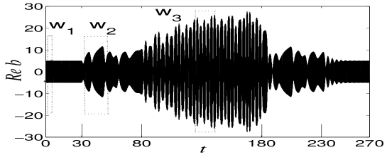
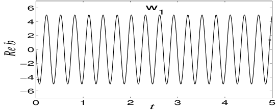
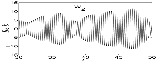
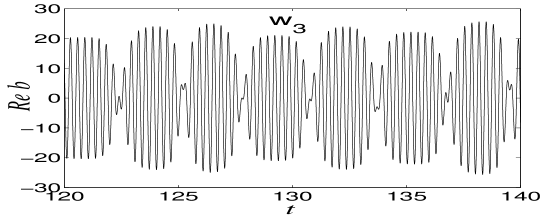
Figure 1:

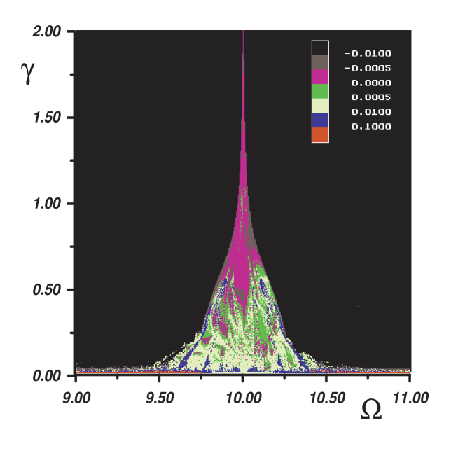
Figure 2:

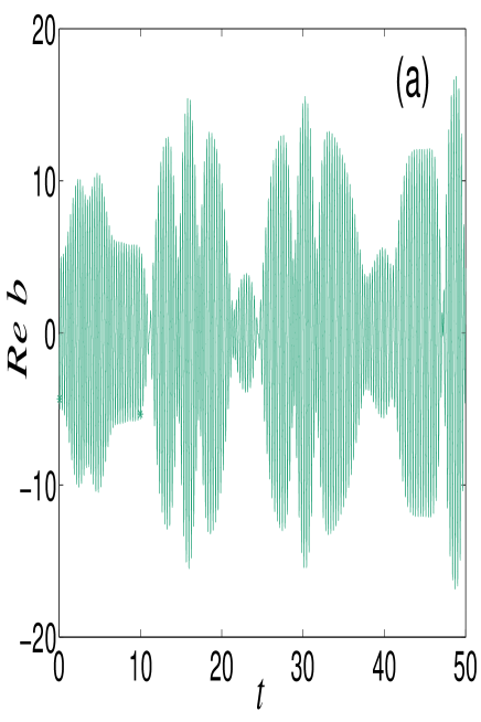
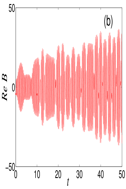
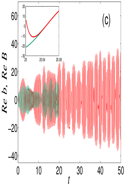
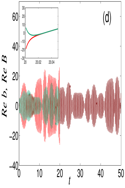
Figure 3:

References

- (1) Minorsky, N. [1962] Nonlinear Oscillations, Van Nostrand, Princeton.
- (2) Eberly, J. H., Narozhny, N. B., & Sanchez-Mondrogon, J. J. [1980] ”Periodic spontaneous collapse and revivalsin a simple quantum model”, Phys. Rev. Lett. 44, 1323-1326.
- (3) Grygiel, K. & Szlachetka, P. [2002] ”Generation of chaotic beats”, Int. J. Bifurcation and Chaos 12, 635-644.
- (4) Cafanga, D. & Grassi, G. [2004] ”A new phenomenon on nonautonomous Chua’s circuits: generation of chaotic beats”, Int. J. Bifurcation and Chaos 14, 1773-1788.
- (5) Cafanga, D. & Grassi, G. [2004] ”Chaotic beats in a modified Chua’s circuits: dynamic behavior and circuit design”, Int. J. Bifurcation and Chaos 14, 3045-3064.
- (6) Cafagna, D. & Grassi, G. [2005] ”On the generation of chaotic beats in simple nonautonomous circuits”, Int. J. Bifurcation and Chaos 15, 2247-2256.
- (7) Mandel, P. & Erneux, T. [1982] ”Amplitude self-modulation of interactivity second-harmonic generation”, Opt. Acta 29, 7-21.
- (8) Peřina, J. [1991] Quantum statistics of linear and nonlinear optical phenomena, Kluwer Academic Publishers, Dordrecht.
- (9) Pikovsky, A., Rosenblum, M., & Kurths, J. [2001] Synchronization - a universal concept in nonlinear sciences, in Cambridge Nonlinear Sciences Series 12 , Cambridge Univ. Press.
- (10) Wolf, A., Swift, J.B., Swinney H.L. & Vastano, J.A. [1985] ”Determining Lyapunov exponents from a time series”, Physica D 16, 285-317.
- (11) K. Pyragas, [1992] ”Continuous control of chaos by self-controlling feedback”, Phys. Lett. A 170, 421-428.