Stokes’ Second Flow Problem in a High Frequency Limit: Application to Nanomechanical -Resonators.

Abstract

Solving the Boltzmann - BGK equation, we investigate a flow generated by an infinite plate oscillating with frequency $\omega$. Geometrical simplicity of the problem allows a solution in the entire range of dimensionless frequency variation $0\leq\omega\tau\leq\infty$, where $\tau$ is a properly defined relaxation time. A transition from viscoelastic behavior of Newtonian fluid ($\omega\tau\rightarrow 0$) to purely elastic dynamics in the limit $\omega\tau\rightarrow\infty$ is discovered. The relation of the derived solutions to microfluidics (high-frequency micro-resonators) is demonstrated on an example of a ”plane oscillator”.

Introduction. During last two centuries, Newtonian fluid approximation was remarkably successful in explaining a wide variety of natural phenomena ranging from flows in pipes, channels and boundary layers to the recently discovered processes in meteorology, aerodynamics , MHD and cosmology. With advent of powerful computers and development of effective numerical methods, Newtonian hydrodynamics remains at the foundation of various design tools widely used in mechanical and civil engineering. Since technology of the past mainly dealt with large ( macroscopic) systems varying on the length/ time-scales $L$ and $T$, the Newtonian fluid approximation, typically defined by the smallness of Knudsen and Weisenberg numbers $Kn=\lambda/L\ll 1$ and $Wi=\tau/T\approx\frac{\lambda}{L}\frac{u}{c}=KnMa\ll 1$, was accurate enough. The length and time-scales $\lambda$ and $\tau\approx\lambda/c$, are the mean -free path and relaxation time, respectively, .

With recent rapid developments in nanotechnology and bioengineering, quantitative description of high-frequency oscillating microflows, i. e. flows where Newtonian approximation breaks down, became an important and urgent task from both basic and applied science viewpoints. Modern micro (nano)- electromechanical devices (MEMS and NEMS), operating in the high- frequency range up to $\omega=O(10^{8}-10^{9}Hz)$ ($Wi=\omega\tau\geq 1$), can lead to small biological mass detection, subatomic microscopy, viscometry and other applications [1]-[3]. The manufactured devices are so small and sensitive that adsorption of even tiny particles on their surfaces leads to detectable response in the resonator frequency peak (shift) and quality ($Q$) factor, thus enabling these revolutionary applications. Since both frequency shift and width of the resonance peak, depend upon properties of the resonator -generated flows, the microresonators may serve as sensors enabling accurate investigation of fundamental processes in microflows.

Often, oscillating flows are a source of new and unexpected phenomena. For example, in a recent study of the high-frequency elctro-magnetic - field - driven nano -resonators ($h\times w\times L\approx 0.2\times\times 0.7\times 10\mu m$) Ekinci and Karabacak , observed a transition in the frequency dependence of inverse quality factor from $1/Q\approx\gamma/\omega\propto 1/\sqrt{\omega}$, expected in the hydrodynamic limit, to $1/Q\propto 1/\omega$ in the high-frequency (kinetic) limit [3]. Since parameter $\gamma\propto W$ is proportional to the energy dissipation rate ($W$) into a surrounding gas, the discovered effect points to the frequency- independent dissipation rate $W$. No quantitative theory describing this transition has been developed.

Recently, Shan et. al. performed a detailed numerical investigation of evolution of the initially prepared viscous shear layer defined by a unidimensional velocity field ${\bf u}(y,0)=u_{0}\cos(k_{0}y){\bf i}$, where ${\bf i}$ is the unit vector in the $x$-direction. A novel transition from purely viscous decay to the viscoelastic dynamics was discovered for $\tau\nu k_{0}^{2}\geq 1$ [4].

In this paper we investigate deviations from Newtonian hydrodynamics, on an example of classic ” Stokes’ Second ” problem of a flow generated by an infinite solid plate oscillating along $x$-axis with velocity $u(y=0,t)=U\cos\omega t$ [5]. First we use the hydrodynamic approximation, derived from kinetic equation by Chen et. al..[6] in the limit $\omega\tau\ll 1$. Then, derivation of equations valid in an infinite range $0<\omega\tau<\infty$ is presented and it is shown that in the high-frequency limit $\omega\tau\rightarrow\infty$, the dissipation rate $W\rightarrow const$. To apply the derived solution to experimental data on nano-resonators, we introduce a model system of plane oscillator and demonstrate the transition in the frequency dependence of the quality factor, in a quantitative agreement with experimental data of in Refs. [4], [5].

The Boltzmann-BGK equation. Interested in the rapidly oscillating flows , where the Navier-Stokes equations break down, we consider the kinetic equation in the relaxation time approximation (RTA):

$$\frac{\partial f}{\partial t}+{\bf v}\cdot\nabla f={\cal C}$$ (1)

In accord with Boltzmann’s H-theorem , the initially non-equilibrium gas must monotonically relax to thermodynamic equilibrium. This leads to the relaxation time anzatz, qualitatively satisfying this requirement:

$${\cal C}\approx-\frac{f-f^{eq}}{\tau(v)}$$ (2)

In thermodynamic equilibrium the left side of kinetic equation is equal to zero and the remaining equation ${\cal C}=0$ has a solution: $f^{eq}=constant\times e^{-\frac{E({\bf p,r})}{\theta}}$ with the temperature $\theta=const$. In the mean -field approximation, valid close to equilibrium where all gradients are small, one replaces the variable $v$ by $\overline{v}\propto\sqrt{T/m}$. Given the mean-free path $\lambda$, we have an estimate $\tau=\lambda/\overline{v}\approx\lambda/c=const$ where $c$ is the speed of sound. In general, the relaxation time can be a non-trivial function of velocity gradients, position in the flow, external fields etc [7]. The equation (1)-(2) is the celebrated Boltzmann BGK equation widely used for both theoretical and numerical (Lattice Boltzmann Method) studies of non-equilibrium fluids [7]. This equation, with

$$f^{eq}=\frac{\rho}{(2\pi\theta)^{\frac{3}{2}}}\exp(-\frac{({\bf v-u})^{2}}{2\theta})$$ (3)

often considered as a generic equation of fluid dynamics, is valid when velocity gradients are not large. It will be shown below that, due to a particular geometry studied in this paper, the largest magnitude of velocity gradient $|\partial_{y}u(0,t)|<U/\delta$ with $\delta\rightarrow\infty$ when $\omega\tau\rightarrow\infty$. Therefore, when the amplitude $U$ is small enough, the typical gradient is small. Moreover, this feature is responsible for the purely elastic response and total disappearence of viscosity from the problem. In turbulence theory this effect is called rapid distortioin (RD) limit.

Chapman-Enskog expansion of BGK. Chen et.al (2003). Multiplying (1),(2) by $v$ and integrating over ${\bf v}$ gives:

$$\frac{\partial u_{i}}{\partial t}+u_{j}\frac{\partial u_{i}}{\partial x_{j}}+\frac{1}{\rho}\frac{\partial}{\partial x_{i}}\rho\sigma_{ij}=0$$ (4)

where the stress tensor, written for $i\neq j$ is:

$$\sigma_{ij}=\overline{(v_{i}-u_{i})(v_{j}-u_{j})}\equiv\int d{\bf v}(v_{i}-u_{i})(v_{j}-u_{j})f({\bf v,x},t)$$ (5)

Usually, evaluation of the stress tensor is a difficult task. The simplified equation (1)-(2) for a single-particle distribution function allows calculation of nonlinear contributions to the momentum stress tensor $\sigma_{ij}=\overline{(v_{i}-u_{i})(v_{j}-u_{j})}-\frac{1}{d}\overline{v^{2}}\delta_{ij}$. In a remarkable paper, Chen et. al. [6], based on thequation (1)-(2), formulated the Chapman-Enskog expansion in powers on dimensionless relaxation time $\epsilon=\tau\partial_{x_{i}}u_{j}$. In this formulation:

$$\nabla=\epsilon\nabla_{1}$$ (6)

$$\frac{\partial}{\partial t}=\epsilon\frac{\partial}{\partial t_{0}}+\epsilon^{2}\frac{\partial}{\partial t_{1}}+\epsilon^{3}\frac{\partial}{\partial t_{2}}+\cdot\cdot\cdot$$ (7)

and the pdf is expanded in powers of $\epsilon$ as:

$$f=f^{(0)}+\epsilon f^{(1)}+\epsilon f^{(2)}+\cdot\cdot\cdot$$ (8)

Substituting these expressions into (1),(2) and equating the terms of the same order in $\epsilon$ results in $f^{(0)}=f^{eq}$ given by (3), and

$$(\frac{\partial}{\partial t_{0}}+{\bf v}\cdot\nabla)f^{(0)}=-\frac{f^{(1)}}{\tau}$$ (9)

$$(\frac{\partial}{\partial t_{0}}+{\bf v}\cdot\nabla)f^{(1)}+\frac{\partial}{\partial t_{1}}f^{(0)}=-\frac{f^{(2)}}{\tau}$$ (10)

etc. The mean of any fluctuating variable is then calculated as :

$$\overline{A({\bf v})}=A^{(0)}+A^{(1)}+A^{(2)}+\cdot\cdot\cdot$$ (11)

where

$$A^{(n)}=\int f^{(n)}A({\bf v}){\bf v}$$

To illustrate the main results and simplify notation in what follows we set the temperature $\theta=const$. The calculation of Chen (2003) gives:

$$f^{(1)}\approx-\frac{\tau}{\theta}f^{(0}S_{ij}[(v_{i}-u_{i})(v_{j}-u_{j})-\frac{({\bf v-u})^{2}}{d}\delta_{ij}]$$ (12)

and

$$f^{(2)}=-2\tau^{2}f^{(0)}[(v_{i}-u_{i})\frac{\partial}{\partial x_{j}}(S_{ij}-\frac{1}{d}\nabla\cdot{\bf u}\delta_{ij})+O((v_{p}-u_{p})(v_{q}-u_{q})S_{pi}S_{qi})]$$ (13)

It is important to stress that the last contribution to the right side of (13) involves even powers of $v-u$ and various products of $S_{ij}$. The result is (Chen (2003)):

$$\sigma_{ij} = 2\tau\theta S_{ij}-2\tau\theta(\partial_{t}+{\bf u}\cdot\nabla)(\tau S_{ij})$$ (14)

$$-4\tau^{2}\theta[S_{ik}S_{kj}-\frac{1}{d}\delta_{ij}S_{kl}S_{kl}]+2\tau^{2}\theta[S_{ik}\Omega_{kj}+S_{jk}\Omega_{ki}]$$

where the rate of strain $S_{ij}=\frac{1}{2}[\frac{\partial u_{i}}{\partial x_{j}}+\frac{\partial u_{j}}{\partial x_{i}}]$ and the vorticity tensor is defined as, $\Omega_{ij}=\frac{1}{2}[\frac{\partial u_{i}}{\partial x_{j}}-\frac{\partial u_{j}}{\partial x_{i}}]$.

The first term in the right side of (14), resulting from the first order Chapman-Enskog (CE) expansion, corresponds to the familiar Navier-Stokes equations for Newtonian fluid and the non-linear (non - Newtonian) corrections, given by the remaining terms, are generated in the next , second, order. The constitutive relation (14) is quite complex and, in general, can be attacked by numerical methods only. However, it is greatly simplified in an important class of simple unidirectional flows.

Stokes’ Second Problem is formulated as follows: The flow of a fluid filling half -space $0\leq y$ is generated by a solid plate at $y=0$ moving along the $x$-axis with velocity $U_{p}(0,t)=U\cos\omega t$. Since velocity components in $y$ and $z$-directions are equal to zero, we have to solve the equations for the $x$-component of velocity field $u(y,t)$ only. Due to geometry of the problem

$$u_{x}\equiv u=u(y,t);~{}~{}u_{y}\equiv v=0;~{}~{}{\bf u}\cdot\nabla=0;~{}~{}\partial_{x}=0$$ (15)

Thus, since $i\neq j$, we are interested in $\sigma_{x,y}$. In this case, the equation of motion corresponding to the stress tensor (14) is very simple:

$$\frac{\partial u}{\partial t}=\nu(1-\tau\frac{\partial}{\partial t})\frac{\partial^{2}u}{\partial y^{2}}$$ (16)

In the limit $\omega\tau\rightarrow 0$, this equation is to be solved subject to the no-slip boundary condition, $u(0,t)=U\cos\omega t;~{}~{}\lim_{y\rightarrow\infty}u(y,t)=0.$ Seeking a solution, satisfying the boundary condition at $y\rightarrow\infty$, as: $u={\cal R}(\phi(y)e^{-i\omega t})$ gives: $\phi=Be^{-\frac{y}{\delta}}$ and in the low frequency limit $Wi=\tau\omega\ll 1$:

$$u(y,t)=Uexp(-\sqrt{\frac{\omega}{2\nu}}(1-\frac{\tau\omega}{2})y)\cos(\omega t-\sqrt{\frac{\omega}{2\nu}}(1+\frac{\tau\omega}{2})y)$$ (17)

In a classic case $\omega\tau=0$, the flow is characterized by a single scale $\sqrt{2\nu/\omega}$ describing both ”penetration depth” and wave-length of transverse waves radiated by the oscillating plate. We can see that the non-newtonian $O(\tau\omega)$ contribution leads to formation of two different length-scales: the $O(\tau\omega)$ increasing penetration depth and by the wave-length decreasing by the same magnitude. This is a qualitatively new feature of a non-newtonian flow. Now we calculate the dissipation rate. The force acting on the unit area of the wall at $y=0$ :

$$\mu(1-\tau\frac{\partial}{\partial t})\frac{\partial u(0,t)}{\partial y}=-U\sqrt{\omega\mu\rho}[\cos(\omega t+\frac{\pi}{4})+\frac{\tau\omega}{2}\cos(\omega t-\frac{\pi}{4})]$$ (18)

is phase-shifted relative to velocity field $u(0,t)=U\cos\omega t$. This result differs from its classic Newtonian counterpart by an $O(\tau\omega/2)$ shift. The mean energy dissipated per unit time per unit are of the plate is calculated if we multiply (18) by $-U\cos\omega t$ and integrate over one cycle with the result:

$$W(\tau,\omega)=\frac{U^{2}}{2}\sqrt{\frac{\omega\mu\rho}{2}}(1+\frac{\tau\omega}{2})>W(0,\omega)$$ (19)

In a simple gas close to thermodynamic equilibrium, the mean-free path $\lambda\approx\frac{1}{\sqrt{2}\Sigma n}\propto\frac{k_{B}T}{d^{2}p}$ where $\Sigma\propto d^{2}$ is a scattering cross-section of the molecules and $d$ is a typical scale of intermolecular interaction.

Large deviations from Newtonian fluid mechanics. Here we somewhat modify the procedure developed by Chen (2003). It is clear that as $\tau\rightarrow 0$, the expansion gives the classic Stokes results for the flow of oscillating plate. Moreover, in the limit $\tau\omega\ll 1$, the second -order in ${\bf S}$ correction to (14) disappears due to the symmetries of the problem defined by (7). The expression (14) includes a time derivative, which for the oscillating flow we are interested in this paper, introduces an additional dimensionless parameter $Wi-\tau\omega$ into expansion. Therefore, the CE expansion is in fact expansion in two dimensionless parameters $Kn=\tau\partial_{y}u$ and $Wi$. As will be shown below, in the simple-geometry oscillating flows, these parameters are quite different : as $\tau\omega\rightarrow\infty$, the second parameter $Kn\rightarrow 0$. Thus, while neglecting the small, $O(\nabla^{2n}u)$ with $n>1$, ”Burnett contributions”, we will attempt to sum up the entire series in $Wi=\tau\omega$ . The Boltzmann equation is:

$$\frac{\partial f}{\partial t}+v_{\alpha}\frac{\partial f}{\partial x_{\alpha}}+\frac{f}{\tau}=\frac{f^{e}}{\tau}$$ (20)

Multiplying (20) by $(v_{i}-u_{i})(v_{j}-u_{j})$ and integrating over $\bf v$, we derive the equation for the stress tensor ( $i\neq j$): :

$$\frac{\partial\sigma_{ij}}{\partial t}+\frac{\sigma_{ij}}{\tau}=-\frac{1}{\rho}\int d{\bf v}(v_{i}-u_{i})(v_{j}-u_{j})v_{\alpha}\frac{\partial f}{\partial x_{\alpha}}$$ (21)

or

$$\frac{\partial\sigma_{ij}}{\partial t}+{\bf u}\cdot\nabla\sigma_{ij}+\frac{\sigma_{ij}}{\tau}=-2\sigma_{i,\alpha}\frac{\partial u_{j}}{\partial x_{\alpha}}-\frac{\partial}{\partial x_{\alpha}}\overline{(v_{\alpha}-u_{\alpha})(v_{i}-u_{i})(v_{j}-u_{j})}-\sigma_{ij}\nabla\cdot{\bf u}$$ (22)

Due to the basic symmetries of the problem (7), this equation is simplified:

$$\frac{\partial\sigma_{ij}}{\partial t}+\frac{\sigma_{ij}}{\tau}=-2\sigma_{i,\alpha}\frac{\partial u_{j}}{\partial x_{\alpha}}-\frac{\partial}{\partial x_{\alpha}}\overline{(v_{\alpha}-u_{\alpha})(v_{i}-u_{i})(v_{j}-u_{j})}$$ (23)

In the unidirectional flow, we are interested in only $\partial_{y}u\neq 0$ and therefore,

$$\sigma_{i,\alpha}\partial_{x_{\alpha}}u=\sigma_{yy}\partial_{y}u$$ (24)

The remaining term in the right side of equation (15) can also be simplified leading to:

$$\frac{\partial\sigma_{y,x}}{\partial t}+\frac{\sigma_{y,x}}{\tau}=-2\theta\frac{\partial u}{\partial y}-\frac{\partial}{\partial y}\overline{v_{y}^{2}(v_{x}-u)}$$ (25)

where $\theta=\sigma_{y,y}=\overline{v_{y}^{2}}=\frac{({\bf v-u})^{2}}{3}$. This equation is formally exact.

Our goal now is to evaluate

$$\Sigma_{ij}=\frac{\partial}{\partial x_{\alpha}}\overline{(v_{\alpha}-u_{\alpha})(v_{i}-u_{i})(v_{j}-u_{j})}=\Sigma_{ij}^{(0)}+\Sigma_{ij}^{(1)}+\Sigma_{ij}^{(2)}+\cdot\cdot\cdot$$ (26)

This can be done readily with relations (3), (11)-(13) derived in Chen (2003). We see that $\Sigma_{ij}^{(0)}=0$ and $\Sigma_{ij}^{(1)}=0$. Evaluated on $f^{(2)}$ from (13)

$$\Sigma_{xy}^{(2)}\approx\tau^{2}\frac{\partial}{\partial y}\overline{v_{y}^{2}(v_{x}-u_{x})^{2}}|_{0}\frac{\partial^{2}u}{\partial y^{2}}\approx\tau^{2}\theta^{2}\frac{\partial^{3}u}{\partial y^{3}}$$ (27)

where $\overline{A}|_{0}=\int f^{0}({\bf v})A({\bf v})d{\bf v}$. It will be shown a’posteriory that in both limits $\tau\omega\rightarrow 0$ and $\tau\omega\rightarrow\infty$, the second order contribution

$$\frac{\Sigma_{ij}^{(2)}}{\theta\partial_{x}u}\approx\frac{\tau^{2}\theta}{\delta^{2}}\rightarrow 0$$ (28)

where $\delta$ is the width of the viscous layer.

As we saw, the high powers of ${\bf S}$ disappear from the second-order relation (14). Let us see that this is a general phenomenon valid to all orders. Let us consider a general $n^{th}$ -order contribution to the stress tensor $\sigma_{x,y}$:

$$\frac{\partial u_{\alpha_{1}}}{\partial x_{\alpha_{3}}}\frac{\partial u_{\alpha_{2}}}{\partial x_{y}}\frac{\partial u_{\alpha_{3}}}{\partial x_{\alpha_{n-1}}}\cdot\cdot\cdot\frac{\partial u_{x}}{\partial x_{\alpha_{n}}}\cdot\cdot\cdot\frac{\partial u_{\alpha_{n-1}}}{\partial x_{\alpha_{2}}}\frac{\partial u_{\alpha_{n}}}{\partial x_{\alpha_{1}}}$$ (29)

where the summation is carried out over the randomly distributed Greek subscripts. By the symmetry

$$\frac{\partial u_{x}}{\partial x_{\alpha_{n}}}\frac{\partial u_{\alpha_{n}}}{\partial x_{\alpha_{1}}}=\frac{\partial u}{\partial y}\frac{\partial v}{\partial x_{\alpha_{n}}}=0$$ (30)

because $v=0$. Denoting $\sigma_{x,y}\equiv\sigma$ we, based on the above considerations obtain equation valid in both low and large-frequency limits:

$$\frac{\partial u}{\partial t}=-\frac{\partial\sigma}{\partial y};\hskip 14.22636pt\tau\frac{\partial\sigma}{\partial t}+\sigma=-\nu\frac{\partial u}{\partial y}$$ (31)

Comparing this result with the equation (16), we conclude that constitutive equation (31) is a resummation of the Chapman-Enskog expansion used in the low-order derivation of (14). Indeed, the Fourier-transform of the second equation in (31) is equal to $(1+i\omega\tau)\sigma(y,\omega)=\nu\frac{du}{dy}$ which in the limit $\omega\tau\rightarrow 0$, coinsides with (16). The equations (31) give:

$$\tau\frac{\partial^{2}u}{\partial t^{2}}+\frac{\partial u}{\partial t}=\nu\frac{\partial^{2}u}{\partial y^{2}}$$ (32)

Boundary conditions. Interested in the limit $\omega\tau>1$, we have to be careful with the choice of boundary conditions (BC). The BC used in this work is $u(0,t)=U(\omega\tau)\cos\omega t=\alpha(\omega\tau)U\cos\omega t$. The ”slip factor $0<\alpha(\omega\tau)\leq 1$ has been recently investigated in detailed numerical simulations where is was shown that for $\omega\tau\leq 1$, $\alpha(\omega\tau)\approx 1$ and it rapidly decreases to $\alpha(\omega\tau)\approx 0.3-0.2$ for $1<\omega\tau\leq 100$ [9]. Dealing with the linear equation, to remove the slip factor from consideration, we can, in principle, introduce the normalized velocity field $u/U(\omega\tau)$, solve equations and then recover $u(y,t)$. Below, we use the no-slip boundary condition.

solution. The solution to equation (32) is found readily: $u={\cal R}[e^{-i\omega t}e^{-\frac{y}{\delta}}]$ with $\frac{1}{\delta}=-(1-i)\sqrt{\frac{\omega}{2\nu}}\sqrt{1-i\omega\tau}$. and:

$$u=Ue^{-\frac{y}{\delta_{-}}}\cos(\omega t-\frac{y}{\delta_{+}})$$ (33)

where

$$1/\delta_{\pm}=(1+\omega^{2}\tau^{2})^{\frac{1}{4}}\sqrt{\frac{\omega}{2\nu}}[\cos(\frac{1}{2}\tan^{-1}(\omega\tau))\pm\sin(\frac{1}{2}\tan^{-1}(\omega\tau))]$$ (34)

In the limit $\omega\tau\rightarrow 0$, this solution tends to the expression (17) derived above. As we see, the non-Newtonian Second Stokes problem can be characterized by two different length-scales, penetration length $\delta_{-}$ and the wave-length $\delta_{+}$. In the limit $\omega\tau\rightarrow\infty$, the penetration length tends to infinity and the dominating dissipation mechanism is the wave generation. (This limits the velocity gradients in this problem). To calculate the force acting on the unit area of the plate, we notice that in accord with the differential equations (31)

$$\sigma(0,t)=\rho\nu\exp(-\frac{t}{\tau})\int_{-\infty}^{t}\frac{\partial u(0,\lambda)}{\partial y}\exp(\frac{\lambda}{\tau})d\frac{\lambda}{\tau}$$ (35)

where $\nu\frac{\partial u(0)}{\partial y}=U(-\frac{\cos\omega t}{\delta_{-}}+\frac{\sin\omega t}{\delta_{+}})$ and

$$\sigma(0,t)=\rho\nu\frac{U}{1+\omega^{2}\tau^{2}}[-\frac{1}{\delta_{-}}(\cos\omega t+\omega\tau\sin\omega t)+\frac{1}{\delta_{+}}(-\omega\tau\cos\omega t+\sin\omega t)]$$ (36)

where $\rho$ is the density of a fluid. To obtain the dissipation rate per unit time per unit area of the plate, we calculate $W=-\overline{u(0,t)\sigma(0,t)}$ averaged over a single cycle. The result is:

$$W(\tau,\omega)=\frac{1}{2}\frac{\mu U^{2}}{1+\omega^{2}\tau^{2}}(\frac{1}{\delta_{-}}+\frac{\omega\tau}{\delta_{+}})$$ (37)

The plot of the normalized dissipation rate as a function of $\omega\tau$ is shown on Fig.1 .

Figure 1: Dissipation rate $2W(\tau,\omega)$ as a function of $\omega$ (expression (16); (arbitrary units).

As $\omega\tau\rightarrow 0$, we recover the previous result $W/\sqrt{\omega}\propto(1+\frac{\omega\tau}{2})$. In the opposite limit $\omega\tau\rightarrow\infty$, the saturation of the curve $W(\omega\tau)$ is predicted. In this range, the kinetic energy of the plate oscillations is mainly dissipated into the wave radiation.

”Plane oscillator”. Consider a massless spring of stiffness $k$ with two infinite plates of height $h$ attached to it. The losses in a spring are neglected and the friction force, acting on the plates, is the only source of energy dissipation. The equation of motion of this ”plane oscillator” driven by a force $R(t)$ is:

$$x_{tt}+\gamma x_{t}+kx=R(t)$$ (38)

where $\gamma x_{t}=\gamma u(0,t)=2\rho\sigma(0,t)/m_{s}$ is the friction force acting on a unit mass ($m_{s}=\rho_{p}h$ ) of a plate surface and the factor 2 accounts for the force acting on both (top and bottom) surfaces of the plate. If the resonance $I(\omega_{0})$ is sharp enough, so that $\delta\omega/\omega_{0}\ll 1$, then we can calculate the damping (friction) force acting on the oscillator using the theory developed above. In Newtonian limit (hereafter, we omit the subscript $0$ ) $\omega\tau\rightarrow 0$, the expression (36) gives $\gamma=\sqrt{\mu\rho\omega/(2m_{s}^{2})}\propto\sqrt{\omega}$ and the quality factor (the definition is given below) $Q\approx\omega/\gamma\propto\sqrt{\omega}$. In the opposite (kinetic) limit $\omega\rightarrow\infty$ and $\tau=const$: $\gamma\rightarrow\mu\omega\tau\sqrt{\frac{\omega}{\nu}}/(m_{s}(1+\omega^{2}\tau^{2})^{\frac{3}{4}})\propto\omega^{0}=const=O(\rho c/m_{s})$

This relation can be understood as follows. We are interested in a somewhat unusual case with the rapidly varying deterministic velocity field $u(0,t)$ and the slow - varying (”frozen”) molecular motion. Thus, the long -time-averaging, giving $\overline{u}=0$, is unphysical and the stress on a plane $y=0$ is calculated by averaging over the plate surface: $\sigma_{xy}=\overline{(u(0,t)+c)_{x}(u(0,t)+c)_{y}}\approx u(0,t)c_{s}$, where $c_{s}$ is the mean velocity ($y$-component) of molecules colliding with solid surface. In this limit, the tangential component of the force acting on a unit surface of a solid (per/unit mass) is: $F_{t}=\frac{\rho c_{s}}{\rho_{s}h}u(0,t)$ and $\gamma=\frac{\rho c_{s}}{\rho_{s}h}$. The former relation, derived here for a rapidly oscillating plate, is similar to the one appearing in a problem of a piston instantaneously accelerated in an ideal gas. Thus, in this limit the inverse quality factor $1/Q=\frac{\gamma}{\sqrt{\omega^{2}-\gamma^{2}}}\approx\gamma/\omega\propto 1/\omega$. For a gas of a given temperature $\rho\propto p$ and $c\propto\sqrt{\theta/m_{mol}}=const$, we have $\frac{1}{Q}\propto p/\omega$

To obtain the relation valid in the entire range of frequency variation we have from (31):

$$\gamma=2\frac{\rho\sqrt{\omega\nu}}{\rho_{p}h(1+\omega^{2}\tau_{p}^{2})^{\frac{3}{4}}}[(1+\omega\tau_{p})\cos(\frac{1}{2}tan^{-1}\omega\tau_{p})-(1-\omega\tau_{p})\sin(\frac{1}{2}tan^{-1}\omega\tau_{p})]$$ (39)

Our goal now is to find the relaxation time $\tau_{p}$ responsible for relaxation to equilibrium in the immediate vicinity of the rapidly oscillating solid plate. In a standard equilibrium situation, when $\lambda$ and $\tau\approx\lambda/c\ll 1/\omega$ are the smallest length and time-scales in the system, the relaxation times in the bulk and in the immediate vicinity of the surface are more or less equal. In a rapidly oscillating flow, we are interested in, this is not so. Indeed, even in the air at normal conditions, the bulk $\tau\approx\lambda/c\approx 10^{-9}sec$ and in the modern microresonators, where $\omega\approx 10^{9}sec^{-1}$, the inequality $\omega\tau\ll 1$ is hardly satisfied. Moreover, in the low pressure devices where $10^{-3}\leq p\leq 10^{3}torr$ , the bulk relaxation time is huge, so that $\tau_{p}$ must be calculated from a theory taking into account strongly non-equilibrium effects. In the absence of such theory, we use the results of experimental data on a driven microbeam obtained by Ekinci and Karabacak [3] who covered an extremely wide range of parameter variation: $10^{0}\leq p\leq 10^{3}torr$, $10^{6}\leq\omega\leq 0.6\cdot 10^{9}sec^{-1}$, $h=2\cdot 10^{-5}cm$. Under the normal conditions for $\omega=0.6\cdot 10^{9}sec^{-1}$ , the observed damping parameter was $\gamma\approx 1.5\cdot 10^{6}sec^{-1}$. (This relation is the result of the measured $1/Q=\gamma/\omega\approx 3\cdot 10^{-3}$ and $\omega_{0}=0.6\cdot 10^{9}sec^{-1}$.) Denoting $x=\omega\tau_{p}$ and introducing a geometric factor $g$ accounting for the geometry differences between theoretical and experimental setups, we have:

$$\frac{g}{4(1+x^{2})^{\frac{3}{4}}}[(1+x)\cos(\frac{1}{2}tan^{-1}x)-(1-x)\sin(\frac{1}{2}tan^{-1}x)]=1$$ (40)

In this paper we considered a case of the simplest possible geometry. In the nano-technological applications the resonator amplitude is $O(10^{-6}cm)$ is much smallest than the smallest linear dimension of the beam (cantelever). Thus, the results presented here may be not too geometry -sensitive and can be readily generalized to different geometries. For example, the solution to the problem of an infinite cylinder oscillating along its axis can be expressed in terms of the Bessel functions leading to $O(1)$ variations of the coefficient in front of (40). Here, to qualitatively illustrate the origins of the geometric factor $g$, we use very simple considerations. As was stated above, mass per unit area of a plate of height $h$ and length $l$ is : $m_{s}=\rho_{p}l^{2}h/l^{2}=\rho_{p}h$. A simple calculation of $m_{s}$ for circular cylinder gives: $m_{s}=\rho a/2$, where $a$ is the radius. In this case, $g_{cyl}\approx 4d_{plate}$. For a beam of height $h$ and width $w$, we have $m_{s}=\rho_{p}\frac{wh}{2(w+h)}$. Thus, the dissipation per unit area may be a relatively universal property [10]. The equation (19), written for a particular magnitude of frequency ($\omega=0.6\cdot 10^{9}sec^{-1}$) and other parameters of experiment of Refs.[3], [10]) has solutions for all $g\geq 3.6$. For example, $g=4$ and $g=6.28$ give $x\approx 1.8$ and $x\approx 4.8$ corresponding to $\tau\approx 2nsec$ and $\tau\approx 8nsec$, respectively. Choosing $g=4$ we, using the experimental data for normal pressure $p=800torr$ as a calibration point take $\tau_{p}(800torr)\approx 2nsec$ [3]. Then, based on kinetic theory, we substitute $\tau_{p}=\frac{1600}{p}nsec$ into (39) and obtain $\gamma$ and quality factor $Q(\omega,p)$ in a good agreement with the results of Ekinci and Karabacak [3] in a wide range of both frequency and pressure variation ($10^{6}\leq\omega\leq 0.6\times 10^{9}Hz;~{}~{}100\leq p\leq 1000torr$. )

In a kinetic limit $\gamma=const$, and introducing $G(x)=[(1+x)\cos(\frac{1}{2}\tan^{-1}x)-(1-x)\sin(\frac{1}{2}\ tan^{-1}x)]/(1+x^{2})^{\frac{3}{4}}$, the relation (39) give: $a\sqrt{\omega}G(x)=1$, where the coefficient $a=a(p,\theta,m_{s},\rho,g)=const$ includes all parameters of the system. It is easy to check, that solution to this equation $x\propto\omega$ defines an asymptotic kinetic time $\tau_{p}=const\neq\tau$ characterizing relaxation to equilibrium in the high-frequency limit $\omega\tau\rightarrow\infty$. Thus, the equilibrium and non-equilibrium (high-frequency) relaxation times may differ by a constant $O(1)$ factor only. The inverse quality factor $1/Q(\omega)\approx\gamma/\omega$, given by (39), is shown on Fig. 2. The most detailed comparison of the results based on relation (39) with experimental data is presented in Ref. 10.

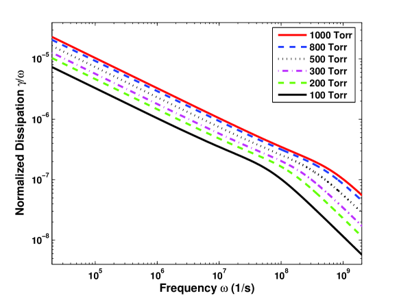
Figure 2: Inverse quality factor $1/Q\approx\gamma/\omega=\frac{4\rho\sqrt{\nu}}{\rho_{p}h\sqrt{\omega}}G(x)\approx 60\sqrt{\frac{p}{800\omega}}G(x)$ (relation (18)) vs frequency $\omega$ in the presure interval $100<p<1000tor$. Relaxation time $\tau_{p}(800torr)=2nsec$. For remaining parameters, see text.

In a dense liquid where $\omega\tau\ll 1$, the relation (39) gives:

$$\gamma=\frac{\rho\sqrt{\omega\nu}}{\rho_{p}\frac{wh}{2(w+h)}}$$ (41)

and in water ($\nu\approx 0.01\frac{cm^{2}}{sec}$, $\rho/\rho_{p}\approx 2$, $\omega\approx 0.6\cdot 10^{9}sec^{-1}$; $h=2\cdot 10^{-5}cm$ and $w=7\cdot 10^{-5}cm$), corresponding to the experimental set up of Ref. 11, we predict $\gamma\approx 1.6\cdot 10^{8}sec^{-1}$ and $Q\approx\frac{\sqrt{\omega^{2}-\gamma^{2}}}{\gamma}\approx 4$, in a good agreement with the data [11].

Summary and conclusions. In this paper a theory of a flow generated by the oscillating plate, valid in a wide range of variation of dimensionless frequency (Weissenberg number) $0\leq\omega\tau\leq\infty$, is presented. The solution to kinetic BGK equation, describing transition between viscoelastic and purely elastic regimes, has been found. The results obtained for a simple ”plane oscillator”, first introduced in this paper, were favorably compared with the outcome of experiments on nanoresonators of Refs. [3],[10] where this transtion has experimentally been observed.

We would like to thank K. Ekinci and D. Karabacak for sharing with us their yet unpublished data on microresonators. We benefited from the most interesting and stimulating discussions with them and R. Benzi, H. Chen, R. Zhang, X. Shan, F. Alexander, S. Succi, I. Karlin and V. Steinberg.

References

[1] R. B. Service, Tipping Scales-Just Barely, Science 312, 683 (2006);
H. G. Craighead, Science 290, 1532 (2000); G. Binning, C.F. Quate, C. Gerber, Phys. Rev. Lett. 56, 930-933 (1986).
[2] A.N. Cleland, M.L. Roukes, Nature 392, 160 (1998); X.M.Huang, C.A. Zorman, M. Mehregani and M.L. Roukes, Nature, 421 496 (2003); K.L. Ekinci, X.M.H. Huang and M.L. Roukes, Appl. phys. Lett. 84, 4469 (2004).
[3] K.L. Ekinci and D. Karabacak, private communication (2006).
[4] Xiaowen Shan H. Chen and R. Zhang, Decay of the Shear Layer, Phys. Rev. E (in press) (2006).
[5]
G. G. Stokes, ”On the effect of the internal friction in fluids on the motion of pendulums.”, Cambr. Phil. Trans., IX, 8 (1851); L..D. Landau and E.M. Lifshitz, Fluid mechanics,
Pergamon Press, Oxford (1959).
[6] H. Chen, S. A. Orszag, I. Staroselsky, and S. Succi, Expanded analogy between Boltzmann kinetic theory of fluids and turbulence, J. Fluid Mechanics, 519 301 (2004)
[7] P.L. Bhatnagar, E. Gross, and M. Krook, Phys. Rev., 94, 511–525 (1954);
S. Chen and G. Doolen. Ann. Rev. Fluid Mech.
30, 329 (1998); H. Chen, S. Kandasamy, S. Orszag, R. Shock,
S. Succi, and V. Yakhot,
Science 301, 633–636, (2003).
[8] Landau, L. D. and Lifshitz, E. M. (1995): Physical
Kinetics, Butterworth/Heinemann.
[9] C. Colosqui and V. Yakhot, ”Lattice Boltzmann Simulations of Second Stokes Flow Problem”, J. Modern Physics (in press); F. Alexander 2006, (private communication).
[10] D. M. Karabacak, V. Yakhot and K. Ekinci, ”High frequency nanofluidics: experimental study with nano-mechanical resonators”, ArXiv, cond-mat/0703230.
[11] S.S. Verbridge, L.M. Bellan, J.M. Parpia and H.G. Craighead, Nano Lett, 6, 2109 (2006).
.