Joint Entropy Coding and Encryption
using Robust Chaos

Abstract

We propose a framework for joint entropy coding and encryption using Chaotic maps. We begin by observing that the message symbols can be treated as the symbolic sequence of a discrete dynamical system. For an appropriate choice of the dynamical system, we could back-iterate and encode the message as the initial condition of the dynamical system. We show that such an encoding achieves Shannon’s entropy and hence optimal for compression. It turns out that the appropriate discrete dynamical system to achieve optimality is the piecewise-linear Generalized Luröth Series (GLS) and further that such an entropy coding technique is exactly equivalent to the popular Arithmetic Coding algorithm. GLS is a generalization of Arithmetic Coding with different modes of operation.

GLS preserves the Lebesgue measure and is ergodic. We show that these properties of GLS enable a framework for joint compression and encryption and thus give a justification of the recent work of Grangetto et al. and Wen et al. Both these methods have the obvious disadvantage of the key length being equal to the message length for strong security. We derive measure preserving piece-wise non-linear GLS (nGLS) and their skewed cousins, which exhibit Robust Chaos. We propose a joint entropy coding and encryption framework using skewed-nGLS and demonstrate Shannon’s desired sensitivity to the key parameter. Potentially, our method could improve the security and key efficiency over Grangetto’s method while still maintaining the total compression ratio. This is a new area of research with promising applications in communications.

1 Introduction

The source coding problem is simple to state: given a source $X$ which is emitting bits of information in the absence of noise, what is the shortest possible way to represent this information? Stated equivalently, how do we achieve the best possible compression of data emitted by a source.

Shannon [1] gave the limit of ultimate data compression by introducing the concept of entropy. Shannon’s entropy of a source is defined as the amount of information content or the amount of uncertainty associated with the source or equivalently, the least number of bits per symbol required to represent the information content of the source without any loss. Shannon did provide a method (Shannon-Fano coding [2]) which achieves this limit as the block-length (number of symbols taken together) for coding increases asymptotically to infinity. Huffman [3] provided what are called minimum-redundancy codes with integer code-word lengths and which achieve Shannon’s Entropy in the limit of the block-length tending to infinity. However, there are problems associated with both Shannon-Fano coding and Huffman coding. As the block-length increases, the number of alphabets exponentially increases, thereby increasing the memory needed for storing and handling. Also, the complexity of the encoding algorithm increases since these methods build code-words for all possible messages of a given length.

In this paper, we address the source coding problem from a different perspective. Since most sources in nature are non-linear, we model the information bits of the source $X$ as measurement bits of a non-linear dynamical system. We treat the bits of information as the symbolic sequence of a non-linear dynamical system. For purposes of simplicity and universality, we want our non-linear dynamical system to be discrete and piece-wise linear. The simplest such system is the Tent map [4].

In the next section, we show how we can use the Tent map to encode binary messages. However, we do not achieve optimality with the standard Tent map. We discuss a method to achieve optimality. We show that this leads us to the Generalized Luröth Series (GLS) map and surprisingly turns out that we have re-discovered the popular Arithmetic Coding algorithm. In Section 4, we discuss the problem of joint compression and encryption. We briefly review recent work in this direction in Section 5 and point out their drawbacks. We aim to provide a motivation for why GLS is a good framework for joint compression and encryption in Section 6. We then derive the equations for measure-preserving piecewise non-linear GLS (nGLS) in Section 7 and discuss the most important feature of these maps namely “Robust Chaos” in Section 8. We then derive their skewed cousins (skewed-nGLS) in Section 9. In Section 10, we indicate how skewed-nGLS may be used in joint entropy coding and encryption and demonstrate Shannon’s desired sensitivity to the key. We also discuss potential advantages of our method and implications on compression efficiency in the same section. We summarize our work with future research directions in Section 11.

2 Entropy coding using the Chaotic Tent Map

We shall now demonstrate how we can use the Tent map, one of the simplest chaotic maps to encode a message. Consider the message $M=`AABABBABAA^{\prime}$ of length $N=10$ bits. We have two partitions in the Tent map, the one pertaining to the alphabet $A$ is $[0,0.5]$ and the other interval $(0.5,1]$ corresponds to $B$. We have the same partitions on the y-axis, as shown in Figure 1. The map consists of linear mappings from the two partitions to $[0,1]$:

$$y = 2x~{}~{}~{}~{}~{}~{}~{}~{}0\leq x<0.5$$

$$= 2-2x~{}~{}~{}0.5\leq x\leq 1$$

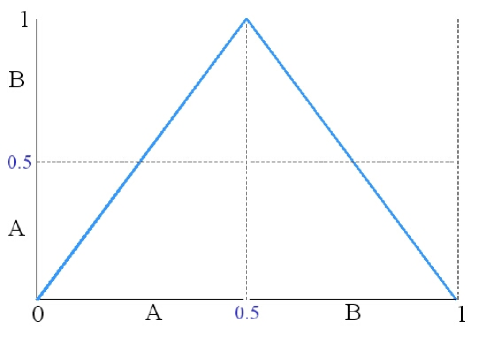
Figure 1: The Tent Map.

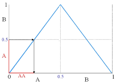
Figure 2: Back iteration on the Tent map to encode message $M=`AABABBABAA^{\prime}$.

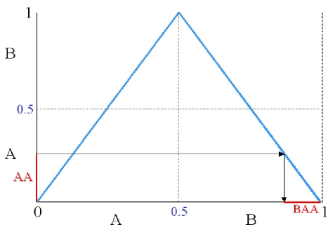
Figure 3: Back iteration on the Tent map to encode message $M=`AABABBABAA^{\prime}$.

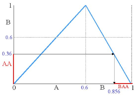
Figure 4: Back iteration on the skewed Tent map to encode message $M=`AABABBABAA^{\prime}$.

To begin coding the message $M=`AABABBABAA^{\prime}$, we begin from the last symbol of the message and back iterate (Figure 2). Since the last symbol is $A$, we begin with the partition $[0,0.5)$ on the y-axis and look at its pre-image. There are two pre-images of this interval corresponding to the two linear maps. Since the previous symbol is also $A$, we take the first pre-image. This would correspond to $[0,0.25)$. We then compute the next back iterate. The symbol is $B$ and hence we take the second pre-image of $[0,0.25)$ which is (0.875, 1] as shown in Figure 3. We keep back-iterating in this fashion until we finally stop (since the message has finite length, this process has to terminate). We end up with an interval $[START,END]$, inside which our initial condition is going to lie. We could choose any real number in this interval as the initial condition. For the sake of simplicity, we choose the mid-point $\frac{START+END}{2}$ as the initial condition. This initial condition is binary coded and transmitted to the decoder.

What we have done effectively is that we have treated the message symbols as the symbolic sequence of the Tent map. We have obtained the initial condition which the decoder forward iterates to yield a trajectory, the symbolic sequence of which is the desired message. Two questions arise:

1. How many bits of the initial condition needs to be transmitted to the decoder?

2. Is such a method optimal in terms of compression?

The answer to the first question is straightforward. It is easy to see that the number of bits needed to transmit is $\lceil-log_{2}(END-START)\rceil+1$ to uniquely distinguish the message from all other messages of the same length. This implies that the number of bits we transmit depends on the length of the final interval ($END-START$). Longer the message, shorter is the interval and hence more bits need to be sent. The second question is more important and the answer is negative. The method is not optimal, in fact, no compression is achieved by this method. This can be easily seen by observing that all possible binary messages of length $N$ bits would get an interval of size $2^{-N}$ units on the real line $[0,1]$ by the encoding we have just described. The number bits needed to transmit the initial condition of a $2^{-N}$ long interval is $N$ bits. Hence no compression is achieved.

2.1 Encoding using the skewed Tent map

We shall now modify our method to make it Shannon optimal. By Shannon optimal, we mean the compression achieved should approach the Shannon’s entropy of the message as the length of the message increases. We notice that the problem we were having is that the standard Tent map is treating all messages as if they were equally likely. This is where the probability model of the source comes into picture. The Tent map treated both $A$ and $B$ as equally likely ($p(A)=p(B)=0.5$ where $p(.)$ denotes first-order probability). This is true only for a perfect random source and we know that a true random sequence is uncompressible. Since most real-world messages that we are interested in storage and transmission are far from random, there is scope for compression. We modify the Tent map to account for the skew in the probabilities of A and B. Specifically, we allocate the intervals, the length of which are equal to the probability of the corresponding alphabet. Thus for the particular example $M=`AABABBABAA^{\prime}$, we first compute the probabilities of $A$ and $B$ as shown in Table 1. Then allocate the range $[0,0.6]$ to $A$ and $(0.6,1]$ to $B$. The encoding proceeds exactly in the same fashion as before (refer to Figure 4). The decoding is also unchanged. However, the probability model of the source has to be now available at the decoder and hence needs to be sent along with the coded message.

Character	Probability	Range
A	$\frac{6}{10}=0.6$	$[0,0.6]$
B	$\frac{4}{10}=0.4$	$(0.6,1.00]$

Table 1: Probability model for the example.

2.2 Shannon Optimality of the modified method

We shall now address the issue of Shannon’s optimality for compression. For the particular example, our method yields an initial condition which requires $11$ bits. The Shannon’s entropy (first-order) for the message is computed as $H=-\sum_{i=0}^{i=1}p_{i}.log_{2}(p_{i})$ where $i=0$ corresponds to the symbol $A$ and $i=1$ to $B$ and $p_{i}$ refers to the probability of the i^th source alphabet. This is found to be $H=0.971$ bits/symbol. This means that for a message of length 10 bits, the optimal number of bits $=10\times H$ which is $9.71$ bits. We don’t seem to achieve optimality for this example. However, with the same probability model for a message of length 1000 bits, our method would transmit 972 bits as opposed to the optimal value of 971 bits. Thus one can see that as the message gets longer, our method approaches Shannon’s optimality.

We make the important observation that the Tent map is a type of Generalized Luröth Series (GLS) [5]. Hence, we shall call this method GLS entropy coding or GLS coding method. We shall now prove theoretically that we achieve Shannon’s optimal limit by showing that GLS coding is equivalent to Arithmetic coding, a popular coding method which is Shannon optimal.

3 GLS coding is equivalent to Arithmetic Coding and hence Shannon Optimal

Let us briefly visit Arithemtic Coding (AC). AC is a popular entropy coding method which has its origins in the early 1960s (Elias and others). However, it gained wide acceptance after the 1979 paper by Rissanen and Langdon [6] who gave a practical implementation of the method. Today, AC is one of the most widely used entropy coding methods owing to its optimality and also improved speed of decoding.

The idea of AC is to first give a unique tag to the entire sequence [7]. This is unlike Huffman coding which gives individual codes to symbols of the message. Since AC codes the entire sequence rather than coding individual symbols, the length of the code-words may not be integers. The tag is then binary coded and transmitted. In AC, there is no need to generate codes for all sequences at a time and hence very efficient for long sequences. Huffman coding has the disadvantage of having to generate code-words for all possible messages of a given length.

The Real line $[0,1)$ is used to generate tags. AC is Shannon optimal without the necessity of blocking. As the length of the message increases, AC comes closer to Shannon’s entropy [7].

3.1 A Binary Example

We shall illustrate the coding method of AC on the same message.

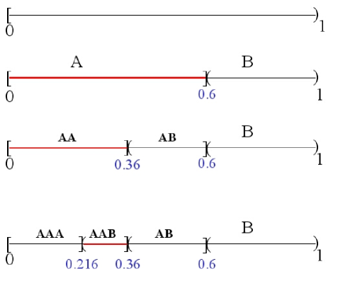
Figure 5: Few iterations of AC encoding of the message $M=`AABABBABAA^{\prime}$

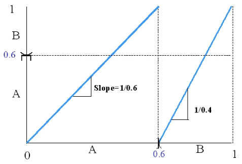
Figure 6: The mode of Generalized Luröth Series (GLS) which is exactly the same as AC. Both methods yield identical intervals for encoding.

First compute the probabilities of $A$ and $B$ as shown in Table 1. Then allocate the range $[0,0.6]$ to $A$ and $(0.6,1)$ to $B$. In order to encode the message $M$, we observe that the first symbol is $A$ and hence the tag will lie in $(0,0.6]$ (refer to the red line marked in Figure 5). We subdivide the interval $[0,0.6]$ into two parts in the ratio $0.6:0.4$, allocating the left one $[0,0.36]$ to $AA$ and $(0.36,0.6]$ to $AB$. Since the second symbol is $A$, the tag will lie in the interval allocated to $AA$ which is $[0,0.36]$. The third symbol is $B$ and so we sub-divide the interval corresponding to $AA$ into two parts in the same ratio ($0.6:0.4$) allocating the left one to $AAA$ ($[0,0.216)$) and the right one to $AAB$ ($(0.216,0.36]$). The tag is going to lie inside $AAB$. We proceed along the same lines until we finally stop (since the message has finite length, this process has to terminate). We end up with an interval $[START,END]$, inside which the tag lies. We could choose any real number in this interval as a tag. For the sake of simplicity, we choose the mid-point $\frac{START+END}{2}$ as the tag. This tag is binary coded and transmitted to the decoder.

We claim that the length of the interval obtained in the above described traditional AC coding is the same as the length of the interval in GLS coding. To see this, we notice that at every iteration of the GLS, the length of the interval we started with is multiplied by the probability of the symbol being encoded to yield us the new length. Thus, at the end of the iterations, the length of the final interval will be $p(A)^{k}p(B)^{N-k}$ where $p(.)$ denotes the first-order probability of the alphabets, ‘$k$’ is the number of $A$-s in the message and $N-k$ is the number of $B$-s in the message for a $N$ bit length message. This is exactly the probability of the message (treating each symbol as independent) and is also the length of the interval for AC. Since the lengths of the final intervals in both AC and GLS coding are the same, the number of bits needed to encode the initial condition will be identical, thus yielding exactly the same compression ratio. Since AC is Shannon optimal, GLS is also Shannon optimal.

It actually turns out that there are different modes of the GLS (which we shall see later) and one of them corresponds to AC. This means that there exists a particular mode of GLS (Figure 6) where not only the length of the final interval is matched with AC, but also the exact interval itself. Note that all modes of GLS are Shannon optimal. Hence, GLS coding can be thought of as a generalization of the AC coding and achieves Shannon’s optimality of compression efficiency.

It is important for us to acknowledge Luca’s work [8] in this context. Luca claims a new method of entropy coding using a chaotic map very similar to ours (their map is exactly the same as AC). However, Luca doesn’t seem to realize that their method is essentially an alternate narrative of AC. They do not make the observation that it is a GLS with a different mode of operation. However, it is important to acknowledge Luca’s contribution in being able to see the coding operation as a back-iteration on an one-dimensional chaotic map (the act of seeing the second dimension in the coding operation is a key thing which they do in their paper).

4 Joint Coding and Encryption: The Problem Statement

The problem that we are now interested in is the following: how to transmit information efficiently and securely from point $A$ to point $B$?

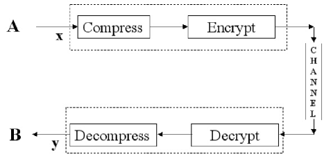
Figure 7: The problem statement.

In order to achieve the above objective, we have to subject the message $x$ to compression in order to come up with a parsimonious representation of its information content. We wish to transmit as little as possible and we know that the best lossless compression theoretically achievable is bounded by Shannon’s Entropy from below. Since we also wish to transmit message $x$ securely, we need to disguise this information by encryption. At the receiver end, we need the corresponding blocks of decryption and decompression to recover the message $y$ (refer to Figure 7). We make the following assumptions:

1. Noiseless source and channel: There is no noise either at the source or at the channel. We will not be needing channel codes.

2. Lossless coding:  All coding will be lossless which implies $x=y$. We shall use the word ‘coding’ to imply compression and ‘decoding’ to imply decompression throughout this paper.

3. Eavesdroppers:  There are eavesdroppers on the channel.

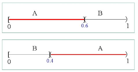
Figure 8: Grangetto’s method [9]: swap between the two modes based on a random key.

5 Joint Entropy Coding and Encryption: Previous Work

In this section, we shall briefly review some previous work on joint entropy coding and encryption.

To the best of our knowledge, there are only two frameworks for joint entropy coding and encryption, that of Grangetto [9] and Wen [10], and both use AC as the entropy coding algorithm. Grangetto proposed randomized AC where at every coding iteration, the intervals of the binary alphabet were switched (or not-switched) based on a random key (Figure 8).

This random switching of the two intervals has the effect of randomizing the location of the final interval $[START,END]$ in which the tag is going to lie. The key consists of 1 bit per coding iteration and hence is essentially as long as the message itself. The key is assumed to be transmitted on a secure channel before the decoding can begin. It can be seen that there is no loss of optimality with respect to the compression ratio in this method.

Wen’s method is a little more complicated where they used key-based interval splitting so that now the intervals allocated to symbols at every iteration are no longer contiguous. The key in this case is also as long as the message. There is a slight loss in optimality of compression ratio which is negligible for long sequences.

Some draw-backs of both methods are as follows:

1. Key-distribution problem:  The key is as long as the message.

2. Why should the method work, if it works?

3. In particular, why should AC be a good choice for such a joint coding and encryption framework? Why not other entropy coding methods like Huffman coding, Shannon-Fano coding etc.?

4. The length of the final interval $[START,END]$ in which the TAG lies is not changed by swapping, only its location on the real line is randomized. This is an important observation which we shall allude to later(“a good disguise should hide one s height.”).

We hope to provide some answers to the above question and also propose a method which has the potential to circumvent some of the above mentioned draw-backs.

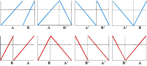
Figure 9: Different modes of GLS. All of these are chaotic, ergodic and Lebesgue measure preserving maps. Grangetto’s method involves swapping between the first mode and the fifth mode (numbering from left to right, top to bottom).

6 Why GLS?

In this section, we wish to provide an answer as to why we think that GLS is potentially a very good candidate for joint entropy coding and encryption.

6.1 GLS a Chaotic, Ergodic, Measure-preserving map

GLS is an ergodic and Lebesgue measure-preserving discrete dynamical system [5]. We intend to make use of these facts for proposing our method of joint coding and encryption.

As previously stated, there are different possible modes of GLS for the binary alphabet case and these are shown in Figure 9. The different modes are obtained by combining the two operations of reversing the map on the partitions and by swapping the two partitions. Grangetto’s method involves swapping between modes 1 and 5 at every coding iteration based on a private key.

Our treatment can be easily extended to larger alphabets. Important properties of the GLS are that it is chaotic, ergodic, Lebesgue measure preserving and Shannon optimal for compression as shown in Section 3. We shall show how these play an important role later.

6.2 Shannon’s remarks from his 1949 masterpiece

We have not yet fully justified why GLS is the ideal candidate for a joint coding and encryption framework. We have to visit Shannon for our argument.

We cite here Shannon’s statements from his famous 1949 paper on secrecy of communications sytems [11] as quoted by Kocarev [12]: “Good mixing transformations are often formed by repeated products of two simple non-commuting operations. Hopf has shown, for example, that pastry dough can be mixed by such a sequence of operations. The dough is first rolled out into a thin slab, then folded over, then rolled, and then folded again, etc. . . . In a good mixing transformation . . . functions are complicated, involving all variables in a sensitive way. A small variation of any one (variable) changes (the outputs) considerably.” Here we wish to make several observations. Shannon is talking about mixing transformation for the purposes of efficient encryption. We believe that he is hinting towards the notion of ergodicity when he refers to mixing. Also, complicated could mean non-linear and involving all variables in a sensitive way could mean chaotic (sensitive dependence on initial conditions indicated by positive Lyapunov exponents). What we are hinting is that Shannon is referring to Chaos and its use in cryptography, 15 years earlier to the coining of the term.

We have shown that AC is nothing but a GLS which is piece-wise linear, chaotic, ergodic and Lebesgue measure preserving discrete dynamical system. We know that it is optimal (achieves Shannon entropy as the length of the message gets longer and longer). We have also seen how good encryption methods need to have properties such as mixing (ergodic), complicated functions (non-linear) and sensitivity to variables (chaotic, positive Lyapunov exponents) as per Shannon’s words. These are best provided by a discrete dynamical system which is chaotic and ergodic. Since our goal is to transmit information efficiently and securely and since both these functions can be achieved by a discrete dynamical system under chaos, why not use a single dynamical system to achieve both? We believe that it is this philosophy that provides a justification for using GLS (or AC) as a framework for joint coding and encryption.

7 nGLS: Measure-preserving Piecewise Non-linear GLS

In this section, we derive a generalization of GLS which is piece-wise non-linear. We call this nGLS. To begin with, we shall consider a binary alphabet standard Tent map.

$$y = 2x~{}~{}~{}~{}~{}~{}~{}~{}~{}~{}0\leq x<0.5$$

$$= 2-2x~{}~{}~{}~{}~{}0.5\leq x\leq 1$$

We re-write this as:

$$\frac{1}{2}y = x~{}~{}~{}~{}~{}~{}~{}~{}~{}~{}0\leq x<0.5$$

$$-\frac{1}{2}y+1 = x~{}~{}~{}~{}~{}~{}~{}~{}~{}~{}0.5\leq x\leq 1$$

We can generalize this as:

$$b_{1}y+c_{1} = x~{}~{}~{}~{}~{}~{}~{}~{}~{}~{}0\leq x<0.5$$

$$b_{2}y+c_{2} = x~{}~{}~{}~{}~{}~{}~{}~{}~{}~{}0.5\leq x\leq 1$$

where $b_{1}=\frac{1}{2}$, $c_{1}=0$, $b_{2}=-\frac{1}{2}$, $c_{2}=1$. We add a non-linear term in $y$,

$$a_{1}y^{2}+b_{1}y+c_{1} = x~{}~{}~{}~{}~{}~{}~{}~{}~{}~{}0\leq x<0.5$$

$$a_{2}y^{2}+b_{2}y+c_{2} = x~{}~{}~{}~{}~{}~{}~{}~{}~{}~{}0.5\leq x\leq 1$$

We set the constraints $y=0$ at $x=0$, $y=1$ at $x=0.5$ and $y=0$ at $x=1$ and simplify the equations to yield:

$$ay^{2}+(\frac{1}{2}-a)y = x~{}~{}~{}~{}~{}~{}~{}~{}~{}~{}0\leq x<0.5$$

$$ay^{2}+(-\frac{1}{2}-a)y+1 = x~{}~{}~{}~{}~{}~{}~{}~{}~{}~{}0.5\leq x\leq 1$$

We can solve for $y$ to get:

$$y = \frac{-1+2a+\sqrt{1-4a+4a^{2}+16ax}}{4a}~{}~{}~{}~{}~{}~{}~{}~{}~{}~{}0\leq x<0.5$$

$$= \frac{1+2a-\sqrt{1-12a+4a^{2}+16ax}}{4a}~{}~{}~{}~{}~{}~{}~{}~{}~{}~{}0.5\leq x\leq 1$$

We call the above equations as $nGLS(a,x)$. It is important to note that as $a\rightarrow 0$, the above equations tend to the standard Tent map. The $nGLS$ family is plotted for a few values of ‘$a$’ in Figure 10.

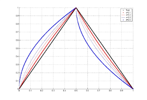
Figure 10: nGLS: piece-wise non-linear GLS for various values of ‘$a$’.

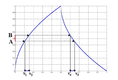
Figure 11: nGLS preserves the Lebesgue measure.

7.1 nGLS preserves the Lebesgue measure

We shall prove that nGLS preserves the Lebesgue measure. In other words, we need to prove:

$$\mu(nGLS^{-1}([A,B]))=\mu([A,B])=B-A$$ (1)

The inverse images of $[A,B]$ are given by Figure 11. These are:

$$x_{1} = aA^{2}+(\frac{1}{2}-a)A.$$

$$x_{2} = aB^{2}+(\frac{1}{2}-a)B.$$

$$x_{3} = aA^{2}+(-\frac{1}{2}-a)A+1.$$

$$x_{4} = aB^{2}+(-\frac{1}{2}-a)B+1.$$

Now,

$$\mu(nGLS^{-1}([A,B])) = (x_{2}-x_{1})+(x_{3}-x_{4}).$$

$$= a(B^{2}-A^{2})+\frac{B-A}{2}+a(-B+A)$$

$$+a(A^{2}-B^{2})+\frac{B-A}{2}+a(B-A).$$

$$= B-A.$$

$$= \mu([A,B]).$$

and hence proved.

7.2 Different modes of nGLS

Similar to the GLS, there are eight different modes of nGLS which are all measure-preserving. We omit plotting these modes here.

Figure 12: nGLS exhibits Robust Chaos in ‘$a$’. The bifurcation diagram is shown above for nGLS for $0<a\leq 0.5$.

Figure 13: Lyapunov exponents of nGLS for $0<a\leq 0.5$. They are found to be positive.

8 nGLS exhibits “Robust Chaos”

Robust Chaos is defined by the absence of periodic windows and coexisting attractors in some neighborhood of the parameter space [13]. Barreto [14] had conjectured that robust chaos may not be possible in smooth unimodal one-dimensional maps. This was shown to be false with counter-examples by Andrecut [15] and Banerjee [13]. Banerjee demonstrates the use of robust chaos in a practical example in electrical engineering. Andrecut provides a general procedure for generating robust chaos in smooth unimodal maps.

As observed by Andrecut [16], robust chaos implies a kind of ergodicity or good mixing properties of the map. This makes it very beneficial for cryptographic purposes. The absence of windows would mean that the these maps can be used in hardware implementation as there would be no fragility of chaos with noise induced variation of the parameters. Recently, we have demonstrated the use of Robust Chaos in generating pseudo-random numbers which passes rigorous statistical randomness tests [17].

nGLS exhibits Robust Chaos in the parameter ‘$a$’ as inferred from the bifurcation diagram in Figure 12.

8.1 Positive Lyapunov exponents

The Lyapunov exponent is experimentally determined for the parameter $0<a\leq 0.5$ and is found to be positive. This is a necessary condition for chaos. Figure 13 shows a plot of Lyapunov exponents for nGLS for the bifurcation parameter $0<a\leq 0.5$. They are found to be positive.

9 Skewed-nGLS

We have so far only considered the symmetric case (the partitions $A$ and $B$ are equal). We now, do similar analysis with a skew and arrive at the following family of maps (we omit the derivation here, it is similar to the derivation of $nGLS$):

$$skewed-nGLS(a,p,x) = \frac{(a-p)+\sqrt{(p-a)^{2}+4ax}}{2a}~{}~{}~{}~{}~{}~{}~{}~{}~{}~{}~{}~{}~{}~{}~{}~{}~{}~{}~{}~{}~{}~{}~{}~{}~{}~{}~{}0\leq x<p$$

$$= \frac{(1+a-p)-\sqrt{(p-a-1)^{2}+4a(1-x)}}{2a}~{}~{}~{}~{}~{}~{}~{}~{}~{}p\leq x\leq 1$$

where $0\leq p\leq 1$ and for a given ‘$p$’, we have $0<a\leq p$. Figure 14 shows the plot of skewed-nGLS for a few values of ‘$p$’ and ‘$a$’. Note that as $a\rightarrow 0$ in each case, the $skewed-nGLS$ tends to the skewed tent-map.

Skewed-nGLS seems to exhibit Robust Chaos as depicted in the bifurcation diagram (Figure 15). We show the bifurcation diagram for values outside the permissible range of ‘$a$’ in Appendix A.

The Lyapunov exponents of skewed-nGLS can be easily derived by observing that the invariant density of the skewed-nGLS is uniform distribution. We can then use the Ergodic theorem to derive the Lyapunov exponents:

$$\lambda(a,p) = \frac{(a+p-1)^{2}log(a+p-1)^{2}-(a-p+1)^{2}log(a-p+1)^{2}}{8a}$$

$$+~{}\frac{(-a+p)^{2}log(-a+p)^{2}-(a+p)^{2}log(a+p)^{2}}{8a}+\frac{1}{2}$$

It can be seen that the Lyapunov exponents are always positive for $0<a\leq k$ where $k=min\{p,1-p\}$.

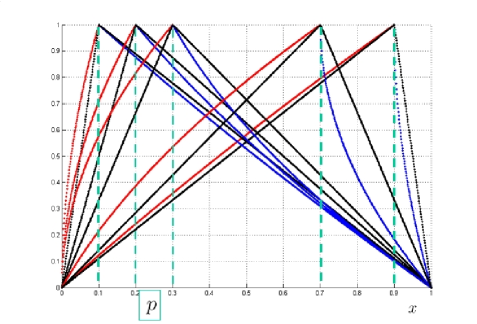
Figure 14: Skewed-nGLS vs. x.

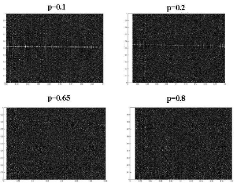
Figure 15: Skewed-nGLS exhibits Robust Chaos as shown by the bifurcation diagram for a few ‘$p$’ values. The white streak for $p=0.1$ and $p=0.2$ disappear when iterated for a long enough time.

10 Joint Entropy Coding and Encryption using Skewed nGLS

We are now ready to propose a new algorithm for joint entropy coding and encryption using skewed-nGLS. We propose using the parameter ‘$a$’ as a private key. Encoding and decoding will be now done with $nGLS(a,p,x)$. The algorithm is exactly the same as before (Section 5.1). Here ‘$p$’ is the source probability of the occurrence of the alphabet $0$ (or $A$) and $1-p$ corresponds to the probability of occurrence of $1$ (or $B$). The key space for ‘$a$’ is $(0,k]$, where $k=min\{p,1-p\}$.

10.1 Shannon’s desired sensitivity of the key parameter ‘$a$’

We shall demonstrate that our method achieves Shannon’s desired sensitivity of the key parameter ‘$a$’. To this end, let us assume a precision of $\delta=10^{-12}$. Consider two keys $a_{1}$ and $a_{2}=a_{1}+\delta$. We chose a random initial condition $IC=0.79193703742704$ and forward iterate $nGLS(a,p=0.5,x)$ for the two keys $a_{1}$ and $a_{2}$ with the same $IC$. We compare the symbolic sequences of the two trajectories.

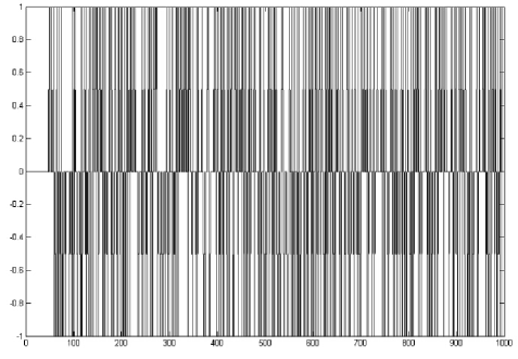
Figure 16: Shannon’s desired sensitivity of the key parameter ‘$a$’. The difference in the symbolic sequences of $nGLS(a_{1},p=0.5,x)$ and $nGLS(a_{2},p=0.5,x)$ is plotted across iterations. As it can be seen, after around 45-47 iterations, they are uncorrelated. $a_{2}=a_{1}+\delta$, $\delta=10^{-12}$.

As it can be seen from Figure 16, the two symbolic sequences are uncorrelated after $45-47$ iterations. For a $\delta=10^{-7}$, they become uncorrelated after 35 iterations. This shows good sensitivity. We have also found that the same is true for various values of ‘$p$’ (not just limited to $p=0.5$). The method we propose is to append $random$ data for the first 50 bits, since it is possible for an eavesdropper to decode correctly up to the first 50 bits with an arbitrary guessed key. We could have a 40-bit key, with a maximum of $k\times 10^{12}$ keys which ‘$a$’ can take. Here the maximum value of ‘$k$’ is $0.5$. The value of the ‘$k$’ depends on ‘$p$’. Remember, $k=min\{p,1-p\}$ and $0<a\leq k$.

10.2 Advantages of our method

1. One time private key (‘$a$’) transmission.

2. Large key space – a maximum of half a billion keys.

3. Sensitivity to key parameter due to Robust Chaos .

4. No windows, no attractive periodic orbits. Well suited for hardware/analog circuit implementation.

5. Overhead is very small $<100$ bits (50 bits of random data + 40 bits of key).

6. Is skewed-nGLS ergodic? We believe it is, though we have no proof at this point. Ergodicity is an important property which would imply mixing or independence, desirable for encryption.

But, we need to find out what happens to the compression ratio?

10.3 Compression ratio efficiency

The compression ratio is not optimal, as it depends on ‘$a$’. For values of ‘$a$’ close to 0 yields us closer to the standard AC and is optimal, but it offers bad encryption. However, we note that the total compression ratio is preserved. The length of the compressed data is scrambled (unlike traditional AC where the length is the same). This implies that two sequences with the same probability may not get the same length. We could swap modes to create efficient scrambling of lengths. The swapping sequence could be based on a key, but unlike Grangetto’s method, we can make the swapping sequence a public key and retain ‘$a$’ as the private key.

11 Summary and Future Research Directions

We have established that GLS coding is equivalent to Arithmetic Coding and hence Shannon optimal. GLS is a chaotic, ergodic and measure-preserving discrete dynamical system. We have provided a motivation for the use of GLS in a framework of joint entropy coding and encryption. We have derived measure preserving piece-wise non-linear GLS (nGLS) and their skewed cousins (skewed-nGLS). nGLS and skewed-nGLS exhibit positive Lyapunov exponents and “Robust Chaos”, both of which are necessary for strong encryption. We have proposed a method for joint compression and encryption using skewed-nGLS which exhibits a reasonably large key space and one-time private key transmission. Shannon s desired sensitivity of keys (due to Robust Chaos) has been demonstrated for this method. We note that the total compression ratio is preserved and the length of the final interval (in which the tag is going to lie) is scrambled.

However, we don’t claim that our method is secure or optimal. We need to perform rigorous cryptanalysis (known plain-text attack, known cipher-text plain-text pair attack, differential cryptanalysis etc.) We also wish to perform analysis on compression ratio distribution of various messages and quantify the loss of optimality of compression ratio and how it can be minimized. Randomizing the length information in an efficient manner while still retaining compression efficiency is important and here swapping modes based on publicly announced sequences would play a role. Issues related to computational precision and decoder complexity need to be addressed. Last but not the least, we need to perform rigorous testing, especially on long sequences.

We hope that we have provided enough hope for utility of Chaos and Robust Chaos in communications by indirectly showing that the popular Arithmetic Coding algorithm is in fact a dynamical system exhibiting Chaos.

Appendix

Appendix A Bifurcation diagrams of $skewed-nGLS(a,p,x)$ for various values of ‘$p$’ for large ranges of ‘$a$’

We shall plot here the various bifurcation diagrams of $skewed-nGLS(a,p,x)$ for various values of ‘$p$’ and for values of of the bifurcation parameter ‘$a$’ outside the range $(0,k]$ where $k=min\{p,1-p\}$.

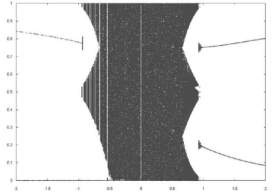
Figure 17: Bifurcation diagram of $nGLS(a,p=0.5,x)$.

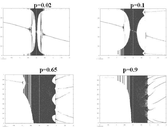
Figure 18: Bifurcation diagram of $nGLS(a,p,x)$ for various values of ‘$p$’. One can notice the white streak in the center of the plot for small values of ‘$p$’ (0.02 and 0.1). This white streak disappears when computed for large number of iterations.

References

- [1] C E Shannon, A Mathematical Theory of Communication, Bell System Technical Journal, vol. 27, pp. 379–423. (1948)
- [2] D Salomon, Data Compression: The Complete Reference, New York: 2nd edn. Springer-Verlag. (2000)
- [3] D A Huffman, A method for the construction of minimum-redundancy codes, Proceedings of the I.R.E., pp. 1098–1102. (sep. 1952)
- [4] K T Alligood, J A Yorke, T D Sauer, Chaos: An Introduction to Dynamical Systems, Springer-Verlag Inc. (1997)
- [5] K Dajani, C Kraaikamp, Ergodic Theory of Numbers, Carus Mathematical Monographs, 29. Mathematical Association of America, Washington, DC. (2002)
- [6] J J Rissanen and G G Langdon, Arithmetic Coding, IBM Journal of Research and Development, vol. 23, no. 2, pp. 146-162. (Mar. 1979)
- [7] K Sayood, Introduction to Data Compression, Morgan Kaufmann. (1996)
- [8] M B Luca, A Serbanescu, S Azou, G Burel, A New Compression Method using a Chaotic Symbolic Approach, www.univ-brest.fr/lest/tst/publications/pdf/comm04_compression_chaos.pdf
- [9] M Grangetto, A Grosso, E Magli, Selective Encryption of JPEG2000 Images by Means of Randomized Arithmetic Coding, IEEE 6th Workshop on Multimedia Signal Processing, Sienam, Italy, pp. 347-350. (Sep. 2004)
- [10] J G Wen, H Kim, J D Vilasenor, Binary Arithmetic Coding Using Key-Based Interval Splitting, IEEE Signal Processing Letters, vol. 13, no. 2. (Feb. 2006)
- [11] C E Shannon, Communication Theory of Secrecy Systems, Bell System Technical Journal, vol. 28, pp. 656-715. (1949)
- [12] I Kocarev, Chaos Based Cryptography, A Brief Overview, IEEE Circuits and Systems Magazine, vol. 1, no. 3, pp. 6-21. (2001)
- [13] S Banerjee, J A Yorke, C Grebogi, Robust Chaos, Physics Review Letters, vol. 80, no. 14. (Apr. 1998)
- [14] E Barreto, B R Hunt, C Grebogi, J A Yorke, From High Dimensional Chaos to Stable Periodic Orbits: The Structure of Parameter Space, Physics Review Letters, vol. 78, no. 24. (Jun. 1997)
- [15] M Andrecut, M K Ali, Robust Chaos in Smooth Unimodal Maps, Physical Review E, vol. 64, no. 025203. (Jul. 2001)
- [16] M Andrecut, M K Ali, Example of robust chaos in a smooth map, Europhyics Letters, vol. 54, no. 3. (May 2001)
- [17] M C Shastry, N Nagaraj, P G Vaidya, The B-Exponential Map: A Generalization of the Logistic Map, and Its Applications In Generating Pseudo-random Numbers, arXiv.org:cs/0607069. (Jul. 2006)